$1.7 trillion life ins. co (13%) cmbs (20%) u.s. commerical mortgage debt outstanding by mit ocw,...
TRANSCRIPT

1
Chapter 20:Chapter 20:
Commercial Mortgage Backed Securities Commercial Mortgage Backed Securities (CMBS)(CMBS)
www.bsscommunitycollege.in www.bssnewgeneration.in www.bsslifeskillscollege.in
1www.onlineeducation.bharatsevaksamaj.net www.bssskillmission.in
WWW.BSSVE.IN

2
20.1. What are CMBS?...20.1. What are CMBS?...•• CMBS are mortgageCMBS are mortgage--backed securities based on backed securities based on commercialcommercialmortgages.mortgages.•• Provide claims to components of the CF of the underlying mortgaProvide claims to components of the CF of the underlying mortgages. ges.
•• Issued in relatively small, homogeneous units, so as to facilitaIssued in relatively small, homogeneous units, so as to facilitate te trading by a large potential population of investors,trading by a large potential population of investors,•• Including those who do not wish (or are unable) to invest largeIncluding those who do not wish (or are unable) to invest large sums of sums of money in any given security. money in any given security.
•• Many CMBS are traded in relatively liquid public exchanges (partMany CMBS are traded in relatively liquid public exchanges (partof the bond market).of the bond market).•• Market for a given individual security is likely to be rather tMarket for a given individual security is likely to be rather thin, but the hin, but the similarity within classes of securities is great enough to allowsimilarity within classes of securities is great enough to allow relatively relatively efficient price discovery and resulting high levels of liquidityefficient price discovery and resulting high levels of liquidity in the market. in the market.
•• Other CMBS are privately placed initially, only traded privatelOther CMBS are privately placed initially, only traded privately (if y (if at all).at all).
www.bsscommunitycollege.in www.bssnewgeneration.in www.bsslifeskillscollege.in
2www.onlineeducation.bharatsevaksamaj.net www.bssskillmission.in
WWW.BSSVE.IN

3
Commercial mortgage loans that are:
– Originated
– Pooled
– Rated by a rating agency
– Sold as a security
20.1. What are CMBS?...20.1. What are CMBS?...
www.bsscommunitycollege.in www.bssnewgeneration.in www.bsslifeskillscollege.in
3www.onlineeducation.bharatsevaksamaj.net www.bssskillmission.in
WWW.BSSVE.IN

4
TrusteeOversees Pool
Servicer(Master Svcr,
Sub-Svcrs)Collects CF
Special ServicerDeals with
defaults, workouts
www.bsscommunitycollege.in www.bssnewgeneration.in www.bsslifeskillscollege.in
4www.onlineeducation.bharatsevaksamaj.net www.bssskillmission.in
WWW.BSSVE.IN

5
CMBS CMBS -- ServicersServicers and Lingo and Lingo ……
• Real Estate Mortgage Investment Conduit (REMIC)(REMIC)
• Pooling and Servicing Agreement (PSA)(PSA)• Servicers: Master, Sub, and Special• Trustee• B-Piece Buyers• Rating Agencies
www.bsscommunitycollege.in www.bssnewgeneration.in www.bsslifeskillscollege.in
5www.onlineeducation.bharatsevaksamaj.net www.bssskillmission.in
WWW.BSSVE.IN
6
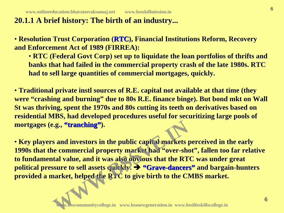
20.1.1 A brief history: The birth of an industry...20.1.1 A brief history: The birth of an industry...
•• Resolution Trust Corporation (Resolution Trust Corporation (RTCRTC), Financial Institutions Reform, Recovery ), Financial Institutions Reform, Recovery and Enforcement Act of 1989 (FIRREA): and Enforcement Act of 1989 (FIRREA):
•• RTC (Federal RTC (Federal GovtGovt Corp) set up to liquidate the loan portfolios of thrifts and Corp) set up to liquidate the loan portfolios of thrifts and banks that had failed in the commercial property crash of the labanks that had failed in the commercial property crash of the late 1980s. RTC te 1980s. RTC had to sell large quantities of commercial mortgages, quickly. had to sell large quantities of commercial mortgages, quickly.
•• Traditional private Traditional private instlinstl sources of R.E. capital not available at that time (they sources of R.E. capital not available at that time (they were were ““crashing and burningcrashing and burning”” due to 80s R.E. finance binge). But bond due to 80s R.E. finance binge). But bond mktmkt on Wall on Wall St was thriving, spent the 1970s and 80s cutting its teeth on deSt was thriving, spent the 1970s and 80s cutting its teeth on derivatives based on rivatives based on residential MBS, had developed procedures useful for securitizinresidential MBS, had developed procedures useful for securitizing large pools of g large pools of mortgages (e.g., mortgages (e.g., ““tranchingtranching””). ).
•• Key players and investors in the public capital markets perceivKey players and investors in the public capital markets perceived in the early ed in the early 1990s that the commercial property market had 1990s that the commercial property market had ““overover--shotshot””, fallen too far relative , fallen too far relative to fundamental value, and it was also obvious that the RTC was uto fundamental value, and it was also obvious that the RTC was under great nder great political pressure to sell assets quickly. political pressure to sell assets quickly. ““GraveGrave--dancersdancers”” and bargainand bargain--hunters hunters provided a market, helped the RTC to give birth to the CMBS markprovided a market, helped the RTC to give birth to the CMBS market. et.
www.bsscommunitycollege.in www.bssnewgeneration.in www.bsslifeskillscollege.in
6www.onlineeducation.bharatsevaksamaj.net www.bssskillmission.in
WWW.BSSVE.IN

7
KeyKey was was devlptdevlpt by bondby bond--rating agencies of the ability to rate the defaultrating agencies of the ability to rate the default--risk of risk of CMBS CMBS tranchestranches::
Recall heterogeneity of investor populationRecall heterogeneity of investor population……•• Bond Bond mktmkt full of full of ““passive investorspassive investors”” (lack time, resources, expertise to assess risk of individual (lack time, resources, expertise to assess risk of individual bonds). Wonbonds). Won’’t invest w/out a reliable measure of default risk.t invest w/out a reliable measure of default risk.•• As with original As with original devlptdevlpt of the 2ndary of the 2ndary mktmkt for residential mortgages in the 1930sfor residential mortgages in the 1930s--50s, a CMBS 50s, a CMBS market could not develop until the investment industry figured omarket could not develop until the investment industry figured out a way to apply traditional ut a way to apply traditional bond bond mktmkt credit risk ratings to CMBS. credit risk ratings to CMBS. •• With RMBS this problem had been solved by the use of mortgage iWith RMBS this problem had been solved by the use of mortgage insurance and pool insurance. nsurance and pool insurance. •• With CMBS it was necessary for bond rating agencies and With CMBS it was necessary for bond rating agencies and investmtinvestmt banks on Wall St to learn banks on Wall St to learn how to quantify the default risk of commercial mortgages. how to quantify the default risk of commercial mortgages. •• This was done via sequential payment and This was done via sequential payment and sequential default assignmentsequential default assignment in the in the tranchingtranching of the of the securities issued from the CMBS pool. securities issued from the CMBS pool. •• When a CMBS When a CMBS tranchetranche obtains a bond rating, investors who know little or nothing aboobtains a bond rating, investors who know little or nothing about ut commercial real estate feel comfortable working under the assumpcommercial real estate feel comfortable working under the assumption that the tion that the default risk of default risk of that that tranchetranche is very similar to the default risk of any other bond with the is very similar to the default risk of any other bond with the same ratingsame rating. . •• This vastly expands the pool of potential investors and makes tThis vastly expands the pool of potential investors and makes the public market for CMBS he public market for CMBS viable.viable.
Traditional Bond Credit Rating LabelsTraditional Bond Credit Rating LabelsApplied to CMBSApplied to CMBS
www.bsscommunitycollege.in www.bssnewgeneration.in www.bsslifeskillscollege.in
7www.onlineeducation.bharatsevaksamaj.net www.bssskillmission.in
WWW.BSSVE.IN

8
20.1.2: Conduits, Seasoned loans, and Risk20.1.2: Conduits, Seasoned loans, and Risk--based capital requirementsbased capital requirements
Two types of loans in CMBS pool at time of IPO:Two types of loans in CMBS pool at time of IPO:•• ““ConduitConduit”” loans,loans,•• ““SeasonedSeasoned”” loans.loans.
Conduit loans:Conduit loans:New loans, issued with intent of being placed into a CMBS pool.New loans, issued with intent of being placed into a CMBS pool.
Seasoned loans:Seasoned loans:Old loans, originally issued by a Old loans, originally issued by a ““portfolio lenderportfolio lender””..
Default risk and prepayment characteristics of new & old loans mDefault risk and prepayment characteristics of new & old loans may differ, hence ay differ, hence credit risk assessment must keep this difference in mind.credit risk assessment must keep this difference in mind.Conduit lenders include:Conduit lenders include:
•• Commercial banks,Commercial banks,•• Investment banks,Investment banks,•• Mortgage banks,Mortgage banks,•• Life Insurance Companies.Life Insurance Companies.
www.bsscommunitycollege.in www.bssnewgeneration.in www.bsslifeskillscollege.in
8www.onlineeducation.bharatsevaksamaj.net www.bssskillmission.in
WWW.BSSVE.IN

9
Why would a portfolio lender such as a LIC want to sell its old Why would a portfolio lender such as a LIC want to sell its old loans into a CMBS pool?loans into a CMBS pool?•• During the 1990s one reason was the establishment of new During the 1990s one reason was the establishment of new ““riskrisk--based capital based capital requirementsrequirements”” (RBC) for depository institutions and life insurance companies.(RBC) for depository institutions and life insurance companies.•• RBC requirements make it necessary for banks and insurance compRBC requirements make it necessary for banks and insurance companies to retain a anies to retain a greater amount of equity backing for investment in types of assegreater amount of equity backing for investment in types of assets that are viewed as ts that are viewed as more risky. more risky. •• RBC requirements view commercial mortgages in the form of wholeRBC requirements view commercial mortgages in the form of whole loans as being loans as being more risky than good quality debt securities. Such loans could bmore risky than good quality debt securities. Such loans could be sold into the CMBS e sold into the CMBS market, and the proceeds of such a sale could be used to buy CMBmarket, and the proceeds of such a sale could be used to buy CMBS securities that S securities that had much lower RBC requirements than the original whole loan. (had much lower RBC requirements than the original whole loan. (TranchingTranching was a was a major means to accomplish this trick.) major means to accomplish this trick.) •• e.g., Suppose for every $1 of equity a LIC could hold $20 worthe.g., Suppose for every $1 of equity a LIC could hold $20 worth of whole of whole commercial mortgages, or $30 worth of investment grade rated boncommercial mortgages, or $30 worth of investment grade rated bonds (including such ds (including such CMBS CMBS tranchestranches). ). The LIC can obtain greater leverage by selling mortgages into The LIC can obtain greater leverage by selling mortgages into CMBS.CMBS.
Traditionally commercial mortgages were almost entirely issued tTraditionally commercial mortgages were almost entirely issued to be held in o be held in portfolio, as there was no major secondary market.portfolio, as there was no major secondary market.Major portfolio lenders were (and are):Major portfolio lenders were (and are):
•• Life Insurance Companies (Life Insurance Companies (LICsLICs))•• Pension Funds (Pension Funds (PFsPFs))
Why do you suppose these were the major types of lenders?Why do you suppose these were the major types of lenders?
www.bsscommunitycollege.in www.bssnewgeneration.in www.bsslifeskillscollege.in
9www.onlineeducation.bharatsevaksamaj.net www.bssskillmission.in
WWW.BSSVE.IN

10
-
20.1.3 The magnitude of the CMBS industry 20.1.3 The magnitude of the CMBS industry
1994 2004
Commercial Banks Life Insurance Cos. CMBS
Savings Associations Pension Funds Other
0
100
200
300
400
500
600
700
800
900
1000
$ B
illio
ns
$727 Billion
Life Ins.Co (23%)
CMBS (5%)
$1.7 Trillion
Life Ins.Co (13%)
CMBS (20%)
U.S. Commerical Mortgage Debt Outstanding
Figure by MIT OCW, adapted from course textbook.www.bsscommunitycollege.in www.bssnewgeneration.in www.bsslifeskillscollege.in
10www.onlineeducation.bharatsevaksamaj.net www.bssskillmission.in
WWW.BSSVE.IN

11
Exhibit 20Exhibit 20--2: CMBS Issuance, U.S., 19902: CMBS Issuance, U.S., 1990--20052005
0
20
40
60
80
100
120
140
160
180
1990 1991 1992 1993 1994 1995 1996 1997 1998 1999 2000 2001 2002 2003 2004 2005
$ Billions
www.bsscommunitycollege.in www.bssnewgeneration.in www.bsslifeskillscollege.in
11www.onlineeducation.bharatsevaksamaj.net www.bssskillmission.in
WWW.BSSVE.IN

12
20.2 CMBS Structure: 20.2 CMBS Structure: TranchingTranching & Subordination& Subordination……
Basic StructureBasic Structure …… A senior/subordinate structure in which the cash flow from the pool of underlying commercial mortgages is used to create distinct classes of securities; the pool is cut up into tranches.
TranchingTranching cash flow claim priority involves two primary dimensions: cash flow claim priority involves two primary dimensions:
•• Loan Retirement. Loan Retirement. Duration / Interest Rate Risk.Duration / Interest Rate Risk.
•• Credit LossesCredit Losses. . Default Risk.Default Risk.
In CMBS it is usually the default risk dimension that is most imIn CMBS it is usually the default risk dimension that is most important (most portant (most commercial mortgages have commercial mortgages have ““prepayment protectionprepayment protection””).).
The opposite is true in RMBS, where duration is the prime concerThe opposite is true in RMBS, where duration is the prime concern, due to n, due to the greater prepayment risk in residential loans (RMBS pools havthe greater prepayment risk in residential loans (RMBS pools have e ““default default protectionprotection””).).
Also, often an Also, often an ““IOIO”” class is class is ““strippedstripped”” off of the other securities (e.g., from off of the other securities (e.g., from the excess of pool loan coupon interest over the Athe excess of pool loan coupon interest over the A--TrancheTranche coupon interest). coupon interest).
www.bsscommunitycollege.in www.bssnewgeneration.in www.bsslifeskillscollege.in
12www.onlineeducation.bharatsevaksamaj.net www.bssskillmission.in
WWW.BSSVE.IN

13
An Aside An Aside …… Prepayment Protection Prepayment Protection in Commercial Mortgages in Commercial Mortgages Due to their history as a prime investment for institutions inteDue to their history as a prime investment for institutions interested in rested in ““maturity maturity
matchingmatching”” (such as (such as LICsLICs), commercial mortgages have traditionally incorporated ), commercial mortgages have traditionally incorporated much more much more ““prepayment protectionprepayment protection”” (aka (aka ““call protectioncall protection””) than residential ) than residential mortgages.mortgages.
Four major types of Four major types of prepayment protectionprepayment protection, listed in order from most to least , listed in order from most to least protective:protective:
1.1. ““Hard LockoutHard Lockout””:: Forbids prepayment prior to loan maturity.Forbids prepayment prior to loan maturity.2.2. ““DefeasanceDefeasance””:: Borrower must purchase TBorrower must purchase T--Bond strips to provide lender with Bond strips to provide lender with
same cash flows as mortgage for remaining life of mortgage.* (Tsame cash flows as mortgage for remaining life of mortgage.* (T--Bond collateral Bond collateral substitutes property collateral, resulting in lower default risksubstitutes property collateral, resulting in lower default risk, hence increased , hence increased value for lender.)value for lender.)
3.3. ““Yield Maintenance ProvisionYield Maintenance Provision””:: Borrower pays a Borrower pays a ““make wholemake whole”” penalty to penalty to lender. Typical requirement would be penalty equal to PV of difflender. Typical requirement would be penalty equal to PV of difference between erence between loan interest and current Tloan interest and current T--Bond interest (for bond of maturity equal to Bond interest (for bond of maturity equal to remaining maturity on loan), with the PV calculated based on Tremaining maturity on loan), with the PV calculated based on T--Bond yield as Bond yield as the discount rate.the discount rate.
4.4. ““Fixed Percentage Penalty PointsFixed Percentage Penalty Points””:: Borrower pays stated percentage over the Borrower pays stated percentage over the OLB on the loan.OLB on the loan.
Note: Many loans mix two or more of the above. (e.g., lockout peNote: Many loans mix two or more of the above. (e.g., lockout period followed by riod followed by points penalty that declines with further age of loan.)points penalty that declines with further age of loan.)
www.bsscommunitycollege.in www.bssnewgeneration.in www.bsslifeskillscollege.in
13www.onlineeducation.bharatsevaksamaj.net www.bssskillmission.in
WWW.BSSVE.IN

14
HARDLOCK-OUT
0 102 to 5 Years
Yield Maintenance Penalty
Fixed Penalty (5-4-3-2-1)
Defeasance
Time: 0 to 10 Years
0-6 Month Free Period N
o Penalty
Common Prepayment Penalties
www.bsscommunitycollege.in www.bssnewgeneration.in www.bsslifeskillscollege.in
14www.onlineeducation.bharatsevaksamaj.net www.bssskillmission.in
WWW.BSSVE.IN

15
0%
10%
20%
30%
40%
50%
60%
70%
80%
90%
100%
1995
.1
1995
.3
1996
.1
1996
.3
1997
.1
1997
.3
1998
.1
1998
.3
1999
.1
1999
.3
2000
.1
2000
.3
2001
.1
2001
.3
2002
.1
DefeasanceYield MaintenanceOther
Prepayment Penalties Over TimeFixed Rate Conduit CMBS
Sources: Bear Stearns, Trepp, LLC
www.bsscommunitycollege.in www.bssnewgeneration.in www.bsslifeskillscollege.in
15www.onlineeducation.bharatsevaksamaj.net www.bssskillmission.in
WWW.BSSVE.IN

16
Typical CMBS Tranching Structure: Sequential Assignment of Credit Losses &Principal Repayments…
$100MMPool of Mortgages
$85MMInvestment Grade CMBS
Aaa/AAAAa/AA
A/ABaa2/BBB
$11 MMNon-Investment
Grade CMBSBa/BB
B/B
$4 MMUnrated CMBS
LowestRisk
Credit
Risk
HighestRisk
LastLoss
Loss Position
FirstLoss
DefaultDefaultRiskRisk
ShortestMaturity
Duration
LongestDur.
FirstPrepay
Repm
tPosition
LastPrepmt
PrepaymentPrepaymentRisk/MaturityRisk/Maturity
www.bsscommunitycollege.in www.bssnewgeneration.in www.bsslifeskillscollege.in
16www.onlineeducation.bharatsevaksamaj.net www.bssskillmission.in
WWW.BSSVE.IN

17
Underlying Pool CharacteristicsUnderlying Pool Characteristics……
Consider a pool consisting of 10 commercial mortgages:Consider a pool consisting of 10 commercial mortgages:•• All 10 mortgages interestAll 10 mortgages interest--only, annual payments in arrears.only, annual payments in arrears.•• All 10 mortgages are nonAll 10 mortgages are non--recourse, with lockouts preventing prepayment.recourse, with lockouts preventing prepayment.•• 5 loans mature in 1 year, 5 in 2 years.5 loans mature in 1 year, 5 in 2 years.•• Each loan par value (OLB) = $10 million.Each loan par value (OLB) = $10 million.•• Each loan coupon (contract) int. rate = 10%. Each loan coupon (contract) int. rate = 10%. •• Collateral value = $142,857,000.Collateral value = $142,857,000.
Therefore,Therefore, Underlying Pool:Underlying Pool:•• Total par value = $100 million, Total par value = $100 million, •• ““Weighted average maturityWeighted average maturity”” (WAM) = 1.5 years.(WAM) = 1.5 years.•• ““Weighted average couponWeighted average coupon”” (WAC) = 10%.(WAC) = 10%.•• LTV ratio = $100,000,000/$142,857,000 = 70%. LTV ratio = $100,000,000/$142,857,000 = 70%.
20.2.1 A simple numerical example of 20.2.1 A simple numerical example of tranchingtranching......
www.bsscommunitycollege.in www.bssnewgeneration.in www.bsslifeskillscollege.in
17www.onlineeducation.bharatsevaksamaj.net www.bssskillmission.in
WWW.BSSVE.IN

18
Loan 1
Loan 2
Loan 3
Loan 4
Loan 5Loan 6
Loan 7
Loan 8
Loan 9
Loan 10
Commercial Mortgage Loans($100m pool; 10, $10m interest-only loans)
Securities(3 tranches, total par value of $100m)
IO Residual Tranche(no par value)
Default Risk Maturity/Duration
Last loss/Lowest Risk
PaymentPriority
"First Loss" /Highest Risk
LongestLife
Tranche ASenior/Invesment
Grade CMBS$75
Tranche BJunior/Non-Investment
Grade CMBS$25m
A Simple Numerical Example of Tranching...
Figure by MIT OCW, adapted from course textbook.www.bsscommunitycollege.in www.bssnewgeneration.in www.bsslifeskillscollege.in
18www.onlineeducation.bharatsevaksamaj.net www.bssskillmission.in
WWW.BSSVE.IN

19
20.2.1 A simple numerical example of 20.2.1 A simple numerical example of tranchingtranching......
CMBS Structure of Securities in the DealCMBS Structure of Securities in the Deal……
Three classes (Three classes (tranchestranches) are created based on the underlying pool, and sold into the ) are created based on the underlying pool, and sold into the bond (CMBS) market:bond (CMBS) market:
A A TrancheTranche is is ““seniorsenior””, , ““investment gradeinvestment grade”” securities:securities:•• Gets retired 1Gets retired 1stst (all five 1(all five 1--yr loans liquidating pmts would go to A).yr loans liquidating pmts would go to A).•• 25%25% credit supportcredit support 25% of pool par value will be assigned credit losses 25% of pool par value will be assigned credit losses (par value lost in default) (par value lost in default) beforebefore A A tranchetranche receives any credit losses (any receives any credit losses (any reduction in par due to default). reduction in par due to default). Effective LTV for A Effective LTV for A tranchetranche = (1= (1--0.25)70% = 0.25)70% = 52.5%. (Underlying properties would have to lose 47.5% of their 52.5%. (Underlying properties would have to lose 47.5% of their value before A value before A tranchetranche gets hit, since it is gets hit, since it is most seniormost senior tranchetranche.).)•• Shorter duration: WAM = (50/75)*1 + (25/75)*2 = 1.33 yrs.Shorter duration: WAM = (50/75)*1 + (25/75)*2 = 1.33 yrs.
••
A
B
IO
Pool
Class Par Value(millions)
WAM(yrs.)
Credit Support Coupon YTM Value as CMBS*
(millions)
$75.00
$24.15
$1.70
$100.85
8%
12%
14%
NA10% (WAC)
NA
10%
8%
NA
NA
0% (1st-loss)
25%
1.50
1.25
2.00
1.33
$100
NA
$25
$75
Figure by MIT OCW, adapted from course textbook.
www.bsscommunitycollege.in www.bssnewgeneration.in www.bsslifeskillscollege.in
19www.onlineeducation.bharatsevaksamaj.net www.bssskillmission.in
WWW.BSSVE.IN

20
B B TrancheTranche is is ““subordinatedsubordinated”” ((““nonnon--investment gradeinvestment grade”” & & ““unratedunrated””) securities:) securities:•• Much riskier than whole loan of 70% LTV, because loss of 47.5% Much riskier than whole loan of 70% LTV, because loss of 47.5% of property of property value would wipe out B value would wipe out B tranchetranche, only cause 25% loss severity (1 , only cause 25% loss severity (1 -- .525/.700) in .525/.700) in loan. loan. •• Longer duration: (WAM = (25/25)*2 = 2.00 yrs.Longer duration: (WAM = (25/25)*2 = 2.00 yrs.
““X X TrancheTranche”” (IO security) has no par value:(IO security) has no par value:•• Based on Based on ““extra interestextra interest”” stripped from A stripped from A tranchetranche (security coupon = 8%, (security coupon = 8%, underlying pool WAC = 10%; underlying pool WAC = 10%; ““notionalnotional”” par val.=$75 million, coupon = 2%, par val.=$75 million, coupon = 2%,
$1.5 million interest per yr.).$1.5 million interest per yr.).•• Subordinated claim on interest in pool (receives only Subordinated claim on interest in pool (receives only residualresidual interest after other interest after other tranchestranches coupons paid, thus exposed to default risk ).coupons paid, thus exposed to default risk ).
A
B
IO
Pool
Class Par Value(millions)
WAM(yrs.)
Credit Support Coupon YTM Value as CMBS*
(millions)
$75.00
$24.15
$1.70
$100.85
8%
12%
14%
NA10% (WAC)
NA
10%
8%
NA
NA
0% (1st-loss)
25%
1.50
1.25
2.00
1.33
$100
NA
$25
$75
Figure by MIT OCW, adapted from course textbook.
www.bsscommunitycollege.in www.bssnewgeneration.in www.bsslifeskillscollege.in
20www.onlineeducation.bharatsevaksamaj.net www.bssskillmission.in
WWW.BSSVE.IN

21
20.2.1 A simple numerical example of 20.2.1 A simple numerical example of tranchingtranching......
Why do you suppose the B Why do you suppose the B TrancheTranche sells at a discount to its par value?...sells at a discount to its par value?...
Why do you suppose the X Why do you suppose the X TrancheTranche ((IOsIOs) requires such a high yield?...) requires such a high yield?...
Figure by MIT OCW, adapted from course textbook.
Par value(millions)
WAM(yrs.)
CreditSupport Coupon YTM
Value as CMBS*(millions)Class
AB
lO NA
Pool $100 1.50 NA 10% (WAC) NA $100.85
$75
$25
NA
1.33
2.00
1.25
8%
10%
NA
8%
12%
14%
25%
0% (1st - loss)
$75.00$24.15
$1.70
Value as CMBS > Par Value
www.bsscommunitycollege.in www.bssnewgeneration.in www.bsslifeskillscollege.in
21www.onlineeducation.bharatsevaksamaj.net www.bssskillmission.in
WWW.BSSVE.IN

22
Now suppose all loans pay as contracted except one of the 2Now suppose all loans pay as contracted except one of the 2--yr loans defaults yr loans defaults in yr.2 paying no interest that year and recovering only $5 millin yr.2 paying no interest that year and recovering only $5 million in ion in foreclosure sale proceeds. What will the ex post CMBS cash flowsforeclosure sale proceeds. What will the ex post CMBS cash flows look like?...look like?...
Tranche (Par, Coupon) Year 1Prin. + Int. = Total CF
Year 2Prin. + Int. = Total CF
Scheduled:Received:
Scheduled:Received:
Scheduled:Received:
Scheduled:Received:
50 + 6 = 5650 + 6 = 56
0 + 2.5 = 2.50 + 2.5 = 2.5
0 + 1.5 = 1.50 + 1.5 = 1.5
50 + 10 = 6050 + 10 = 60
25 + 2 = 2725 + 2 = 27
25 + 2.5 = 27.520 + 2.0 = 22.0
0 + 0.5 = 0.50 + 0.0 = 0.0
50 + 5 = 5545 + 4 = 49
A (75, 8 %)
B (25, 10 %)
10 (NA)
Pool (100, 10 %)
Par value(millions)
WAM(yrs.)
CreditSupport Coupon YTM
Value as CMBS*(millions)
RealizedYld. (IRR)**Class
AB
lO NA
Pool $100 1.50 NA 10% (WAC) NA $100.85 NA
$75
$25
NA
1.33
2.00
1.25
8%
10%
NA
8%
12%
14%
25%
0% (1st - loss)
$75.00$24.15
$1.70
8%
0.75%
-11.79%
Figure by MIT OCW, adapted from course textbook.www.bsscommunitycollege.in www.bssnewgeneration.in www.bsslifeskillscollege.in
22www.onlineeducation.bharatsevaksamaj.net www.bssskillmission.in
WWW.BSSVE.IN

23
20.3 CMBS Rating and Yields20.3 CMBS Rating and Yields……Recall that Recall that keykey to wellto well--functioning liquid public market in CMBS is ability of functioning liquid public market in CMBS is ability of distant, passive investors, who have no local real estate expertdistant, passive investors, who have no local real estate expertise, to feel confident ise, to feel confident about the magnitude of default risk in the securities they are babout the magnitude of default risk in the securities they are buying. uying.
NeedNeed creditcredit--ratingrating from an established bond rating agency. from an established bond rating agency.
Bond Credit RatingBond Credit Rating……An An objective and expert assessmentobjective and expert assessment of the approximate magnitude of of the approximate magnitude of default riskdefault risk..
•• In principle, any two bonds with the same credit rating (from tIn principle, any two bonds with the same credit rating (from the same he same agency) should have similar default risk agency) should have similar default risk
Highest quality (investment grade)
High quality (investment grade)
Medium quality (speculative grade)
Poor quality, some issues in default (speculative to "junk"grades)
Too little information or too risky to rate (generally "junk"grade)
Rating
AaaAa
ABaaBaBCaa &lower
Unrated Unrated
lowerCCC &BBBBBBA
AAAAA
MeaningMoody's S&P
Figure by MIT OCW, adapted from course textbook.www.bsscommunitycollege.in www.bssnewgeneration.in www.bsslifeskillscollege.in
23www.onlineeducation.bharatsevaksamaj.net www.bssskillmission.in
WWW.BSSVE.IN

24
Notes1. Class F accrues interest at a rate equal to the weighted average net mortgage rate
Proceeds ($) Collateral Balance 1,000,000,000
Bond Balance 1,000,000,000
Bond Proceeds 1,040,778,425
Expenses 9,000,000
Net Profit 31,778,425
Yield Yield Frequency Semi-Annual
Yield Day Count 30/360
WA Yield on Bonds 5.19%
WA Spread (bp) 115.34
Average Life (yrs) 9.02
Capital Structure A B C D E F G H I J K L M
Class Rating
Sub Level(%) Balance ($)
Coupon(%)
Price(%)
Yield(%)
Spread (bp)
Bench-mark
Ave. Life (yrs)
Principal Window (mos)
Pricing Scenario
Bond Proceeds ($)
A1 AAA/Aaa 17.000 171,208,000 4.16 100.21 4.12 30.0 S 5.70 116 0 171,559,792
A2 AAA/Aaa 17.000 658,792,000 4.94 100.49 4.90 32.0 S 9.71 1 0 662,045,156
B AA/Aa2 14.000 30,000,000 5.01 100.50 4.97 39.0 S 9.71 1 0 30,149,951
C A/A2 10.500 35,000,000 5.11 100.51 5.07 49.0 S 9.71 1 0 35,178,014
D A-/A3 9.000 15,000,000 5.19 100.52 5.15 57.0 S 9.71 1 0 15,077,365
E BBB/Baa2 6.500 25,000,000 5.47 100.54 5.43 85.0 S 9.71 1 0 25,135,433
F(1) BBB-/Baa3 5.500 10,000,000 5.80 100.43 5.78 120.0 S 9.71 1 0 10,042,815
G BB+/Ba1 4.000 15,000,000 5.24 83.03 7.82 365.0 T 9.71 1 0 12,454,629
H BB/Ba2 3.500 5,000,000 5.24 80.14 8.32 415.0 T 9.71 1 0 4,006,954
J BB-/Ba3 3.000 5,000,000 5.24 70.01 10.27 610.0 T 9.71 1 0 3,500,531
K B+/B1 2.500 5,000,000 5.24 60.67 12.42 825.0 T 9.71 1 0 3,033,722
L B/B2 2.000 5,000,000 5.24 57.80 13.17 900.0 T 9.71 1 0 2,890,186
M B-/B3 1.750 2,500,000 5.24 53.41 14.42 1025.0 T 9.71 1 0 1,335,196
N NR/NR -- 17,500,000 5.24 27.08 27.00 2282.8 T 9.71 1 0 4,738,836
X AAA/Aaa -- 1,000,000,000 W 5.96 6.50 250.0 T 8.88 114 100CPY 59,629,845
20.3.2 Credit rating & CMBS structure: 20.3.2 Credit rating & CMBS structure: realreal--worldworld eexample from Morganxample from Morgan--Stanley Stanley
Based on the following underlying pool and bond market yieldsBased on the following underlying pool and bond market yields……
www.bsscommunitycollege.in www.bssnewgeneration.in www.bsslifeskillscollege.in
24www.onlineeducation.bharatsevaksamaj.net www.bssskillmission.in
WWW.BSSVE.IN

25
Treasury Curve 12/29/2003 (%)
2 yr 1.85
5 yr 3.22
10 yr 4.23
30 yr 5.04
Swap Spreads 12/29/2003 Bps
2 yr 29.50
5 yr 40.75
10 yr 39.00
30 yr 31.25
Deal
Coll. Cut-off Date 01/01/2004
Dated Date 01/01/2004
First Payment Date 02/15/2004
Pricing Date 01/13/2004
Settlement Date 02/01/2004
Pay Frequency Monthly
Collateral Characteristics
Collateral Type No. of Loans
Principal Balance ($)
Gross Coupon
Servicing Fee WAC Seasoning Orig. Amort Orig. Term
Fixed Rate 100 1,000,000,000 5.90% 10 bps 5.80% 4 mos 360 mos 120 mos
Underlying Pool:Underlying Pool:
Bond Market Yield Curve, & Swap spreadsBond Market Yield Curve, & Swap spreads……
www.bsscommunitycollege.in www.bssnewgeneration.in www.bsslifeskillscollege.in
25www.onlineeducation.bharatsevaksamaj.net www.bssskillmission.in
WWW.BSSVE.IN

26
•• Obviously, this CMBS structure is considerably more complex Obviously, this CMBS structure is considerably more complex than our previous highly simplified examplethan our previous highly simplified example
•• Market yields reflect default risk (credit rating), as well as Market yields reflect default risk (credit rating), as well as maturity in some cases (reflecting yield curve). maturity in some cases (reflecting yield curve).
•• Yields are quoted as spread to 10Yields are quoted as spread to 10--yr Tyr T--Bonds for the higher Bonds for the higher yield (nonyield (non--investment grade) investment grade) tranchestranches. In the past it was . In the past it was common to quote yields for all bond common to quote yields for all bond tranchestranches/classes as /classes as spreads to Treasuries. Today, yields for higherspreads to Treasuries. Today, yields for higher--rated rated tranchestranchesare commonly quoted as spreads to similarare commonly quoted as spreads to similar--maturity maturity ““Swapped Swapped LIBORLIBOR””, a fixed, a fixed--interestinterest--rate reflecting LIBOR risk (slight rate reflecting LIBOR risk (slight default risk, illiquidity risk comparable to CMBS AAA default risk, illiquidity risk comparable to CMBS AAA tranchestranches).).
20.3.2 Credit rating & CMBS structure: 20.3.2 Credit rating & CMBS structure: realreal--worldworld eexample continued xample continued ……
www.bsscommunitycollege.in www.bssnewgeneration.in www.bsslifeskillscollege.in
26www.onlineeducation.bharatsevaksamaj.net www.bssskillmission.in
WWW.BSSVE.IN
27
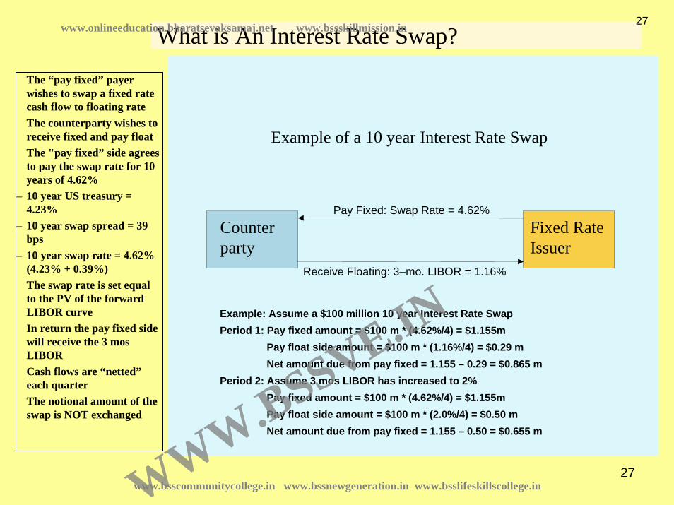
What is An Interest Rate Swap?
Pay Fixed: Swap Rate = 4.62%
Receive Floating: 3–mo. LIBOR = 1.16%
Counterparty
Fixed Rate Issuer
The “pay fixed” payer wishes to swap a fixed rate cash flow to floating rateThe counterparty wishes to receive fixed and pay floatThe "pay fixed” side agrees to pay the swap rate for 10 years of 4.62%
– 10 year US treasury = 4.23%
– 10 year swap spread = 39 bps
– 10 year swap rate = 4.62% (4.23% + 0.39%)The swap rate is set equal to the PV of the forward LIBOR curveIn return the pay fixed side will receive the 3 mos LIBORCash flows are “netted”each quarterThe notional amount of the swap is NOT exchanged
Example of a 10 year Interest Rate Swap
Example: Assume a $100 million 10 year Interest Rate SwapPeriod 1: Pay fixed amount = $100 m * (4.62%/4) = $1.155m
Pay float side amount = $100 m * (1.16%/4) = $0.29 mNet amount due from pay fixed = 1.155 – 0.29 = $0.865 m
Period 2: Assume 3 mos LIBOR has increased to 2%Pay fixed amount = $100 m * (4.62%/4) = $1.155mPay float side amount = $100 m * (2.0%/4) = $0.50 mNet amount due from pay fixed = 1.155 – 0.50 = $0.655 m
www.bsscommunitycollege.in www.bssnewgeneration.in www.bsslifeskillscollege.in
27www.onlineeducation.bharatsevaksamaj.net www.bssskillmission.in
WWW.BSSVE.IN

28
Prepays and R
ecoveries
Loss
es
1.64%
0.86%
Class A–1
Class A–2
AAA/Aaa 4.16%
AAA/Aaa 4.94%
0.79%Class B
Class C
Class D
Class E
AA/Aa2 5.01%
A/A2 5.11%
A–/A3 5.19%
BBB/Baa2 5.47%
18
BBB–/Baa3 5.80%Class F
0.69%
0.61%
0.33%
Class G BB+/Ba1 5.24%
Class H BB/Ba2 5.24%
Class J BB–/Ba3 5.24%
Class K–N B+/B1 to NR 5.24%
0.56%
0.56%
0.56%
0.56%
Bond Coupon Excess Interest
Class X
WAC = 5.80%
– IO = Interest Only security, no principal amount
– WAC = weighted average coupon
– IOs created by stripping interest from a CMBS deal’s various tranches (yellow)
– Size coupons on P&I bonds to create as close as possible to par value bonds as possible
– Difference between bond coupon and WAC of mortgage pool is “excess interest”
– Rated AAA by rating agencies because of seniority in the deal’s cash flow
– IOs are risky bonds –exposed to defaults and to prepayments
TrancheTranche coupons <= Pool couponcoupons <= Pool coupon
I.G. coupons target sales @ parI.G. coupons target sales @ par
www.bsscommunitycollege.in www.bssnewgeneration.in www.bsslifeskillscollege.in
28www.onlineeducation.bharatsevaksamaj.net www.bssskillmission.in
WWW.BSSVE.IN

29
20.3.2 Credit rating & CMBS structure... 20.3.2 Credit rating & CMBS structure... AA Recent CMBS Deal Recent CMBS Deal [[ExhExh. 20. 20--9]9]
Multiple Multiple AAA AAA tranchestranches
High High yield yield tranchestranches
ClassAmount
($Mil)Rating
(Moody's)Rating(S&P)
Subord.(%)
Coupon(%)
Dollar Price
Yield(%)
Avg. Life(Years)
Spread(bp)
A-1 75.150 Aaa AAA 20.00 4.914 100.249 4.801 2.99 S+10A-1A 231.768 Aaa AAA 20.00 8.68A-2 50.000 Aaa AAA 20.00 5.126 100.549 5.007 4.97 S+23A-3-1FL 75.000 Aaa AAA 20.00 L+24 100.000 6.47 L+24A-3-1 78.000 Aaa AAA 20.00 5.251 100.547 5.169 6.47 S+35A-3-2 50.000 Aaa AAA 20.00 5.253 100.545 5.175 6.66 S+35A-AB 75.000 Aaa AAA 20.00 5.178 100.549 5.102 6.91 S+27A-4A 527.250 Aaa AAA 30.00 5.230 100.548 5.186 9.57 S+28A-4B 75.322 Aaa AAA 20.00 5.284 100.546 5.243 9.81 S+33A-J 129.549 Aaa AAA 11.63 5.446 100.547 5.305 9.89 S+39
B 30.938 Aa2 AA 9.63 5.495 100.548 5.357 9.96 S+44C 11.601 Aa3 AA- 8.88 5.513 100.384 5.397 9.97 S+48D 25.137 A2 A 7.25 5.513 99.855 5.467 9.97 S+55E 13.535 A3 A- 6.38 5.513 99.181 5.557 9.97 S+64F 19.335 Baa1 BBB+ 5.13 5.513 97.697 5.777 10.31 S+85G 11.602 Baa2 BBB 4.38 5.513 96.624 5.943 10.87 S+100
H 17.402 Baa3 BBB- 3.25 5.513 92.296 6.513 11.62 S+155J 3.867 Ba1 BB+ 3.00 12.06K 7.734 Ba2 BB 2.50 12.57L 5.801 Ba3 BB- 2.13 13.12M 5.801 B1 B+ 1.75 14.12N 3.867 B2 B 1.50 14.56O 5.801 B3 B- 1.13 14.85P 17.403 NR NR 0.00 17.99X-1(IO) 1,546.863* Aaa AAA 0.043 0.481 7.653 8.46 T+325X-2(IO) 1,502.744* Aaa AAA 0.233 0.704 5.040 6.08 T+70X-Y(IO) 139.729* Aaa AAA 9.10* Notional AmountSource: Commercial Mortgage Alert, October 14, 2005.
Morgan Stanley Capital I Trust, 2005-IQ10
InvstInvst. . grade grade bonds: bonds: BBB and BBB and aboveabove
Mezzanine Mezzanine tranchestranches
No coupon or No coupon or yldyld shown shown →→ bbonds are privately onds are privately placed. placed.
www.bsscommunitycollege.in www.bssnewgeneration.in www.bsslifeskillscollege.in
29www.onlineeducation.bharatsevaksamaj.net www.bssskillmission.in
WWW.BSSVE.IN

30
The new Super-Senior AAA’s…Old schoolOld school
AAA87% of
deal
S+24
New school—Super/SeniorNew school—Super/Senior
AA—NR13.0% of deal
AAA80% of
deal
S+22
AA—NR13.5% of deal
Subordinate AAA7.0%S+26
Blended spread on the AAA’s in the Super-senior scenario is better than what you could sell in the traditional AAA structure
The increased credit support of the super senior (20% vs. 13%) structure has alleviated credit concerns surrounding the “frothiness” of the current lending environment as well the decline in credit support levels
20.00%
13.00%13.00%
Subordination
Blended spread on most senior 87% of deal: S+24
Blended spread on most senior 87% of deal: S+23
8CR
ED
IT
SU
PP
OR
TL
EV
EL
S
www.bsscommunitycollege.in www.bssnewgeneration.in www.bsslifeskillscollege.in
30www.onlineeducation.bharatsevaksamaj.net www.bssskillmission.in
WWW.BSSVE.IN

31
The The creditcredit--rating rating a CMBS a CMBS tranchetranche receives is a function of the nature & receives is a function of the nature & risk of the underlying mortgage pool, plus the risk of the underlying mortgage pool, plus the tranchetranche’’ss credit supportcredit support ……•• e.g., a mortgage pool consisting of loans that have relatively e.g., a mortgage pool consisting of loans that have relatively low and homogeneous LTV low and homogeneous LTV ratios will not need as much credit support for a given creditratios will not need as much credit support for a given credit--rating. Therefore, a larger rating. Therefore, a larger proportion of the securities issued from such a pool can have hiproportion of the securities issued from such a pool can have higher creditgher credit--ratings, which ratings, which means lower yields, thereby enabling the overall CMBS issue to omeans lower yields, thereby enabling the overall CMBS issue to obtain a higher average price btain a higher average price and greater total proceeds.and greater total proceeds.
•• Holding the quality of the underlying mortgage pool constant, gHolding the quality of the underlying mortgage pool constant, greater credit support will reater credit support will result in a higher rating for a given result in a higher rating for a given tranchetranche. .
•• For example, an underlying pool with good quality information aFor example, an underlying pool with good quality information and a 60% LTV ratio might nd a 60% LTV ratio might require only 15% credit support for a AAA rating, enabling 85% orequire only 15% credit support for a AAA rating, enabling 85% of the issuef the issue’’s total par value s total par value to go into senior to go into senior tranchestranches..
•• In contrast, a more heterogeneous pool with an average LTV ratiIn contrast, a more heterogeneous pool with an average LTV ratio of 75% and some o of 75% and some questionable appraisals might require 45% credit support for a Aquestionable appraisals might require 45% credit support for a AA rating, allowing only 55% A rating, allowing only 55% of the pool to be sold at a highof the pool to be sold at a high--priced senior level. priced senior level.
•• It is the job of the bondIt is the job of the bond--rating agency to figure out how much credit support is required rating agency to figure out how much credit support is required for for a given credita given credit--rating for each rating for each tranchetranche in a CMBS issue. The CMBS issuer works with the in a CMBS issue. The CMBS issuer works with the rating agency in an iterative security design process to developrating agency in an iterative security design process to develop the structure of the issue. the structure of the issue.
•• For example, if the rating agency requires 35% credit support fFor example, if the rating agency requires 35% credit support for a AAA rating and 30% for or a AAA rating and 30% for a AA rating, it is then up to the CMBS issuer to decide whether a AA rating, it is then up to the CMBS issuer to decide whether to structure the senior to structure the senior tranchetrancheas a AAAas a AAA--rated rated tranchetranche containing 65% of the pool, or as a AAcontaining 65% of the pool, or as a AA--rated rated tranchetranche containing 70% containing 70% of the pool.of the pool.
www.bsscommunitycollege.in www.bssnewgeneration.in www.bsslifeskillscollege.in
31www.onlineeducation.bharatsevaksamaj.net www.bssskillmission.in
WWW.BSSVE.IN

32
Bond buyers draw a sharp distinction between investmentBond buyers draw a sharp distinction between investment--grade and highgrade and high--yieldyield
Source: JPMorgan Fleming
40
45
50
55
60
65
70
AAA AA A A- BBB BBB- BB+ BB BB- B+ B B- CCC NRTranche Rating
0
200
400
600
800
1000
1200Loan-to-value ratio Spread
High-YieldCMBS
Investment-GradeCMBS
Cumulative Loan-to-value ratio
www.bsscommunitycollege.in www.bssnewgeneration.in www.bsslifeskillscollege.in
32www.onlineeducation.bharatsevaksamaj.net www.bssskillmission.in
WWW.BSSVE.IN

33
Credit Enhancement
Basic Formula: Foreclosure Frequency X Loss Severity = Loss Coverage
The loss coverage implied by this formula must be provided by credit enhancement.
Example: Consider a pool of mortgages that the issuers want to qualify for a Aa2 / AA(double-A) rating.The rating agency decides on a sustainable cash flow, then applies the debtservice coverage ratio that results, say 1.25.If a portfolio were subjected to a double-A level recession (for point ofreference, a double-A recession is comparable to the dislocations in the NewEngland real estate market in 1989-1992), it might experience:
Foreclosure Frequency of 50%
Loss Severity on the sale of foreclosed property of 50%
Then 0.5 X 0.5 = 0.25 = 25%
This portfolio thus requires 25% credit enhancement to qualify the mortgages with a 1.25DSCR for an Aa2/AA rating.
NOTE: In RTC bonds, total credit enhancement often included several components,e.g.,Cash reserve fund + Overcollateralization + Subordination (after A-ratedclasses)
How the credit How the credit rating agencies rating agencies decide on the decide on the amount of credit amount of credit support requiredsupport required……
www.bsscommunitycollege.in www.bssnewgeneration.in www.bsslifeskillscollege.in
33www.onlineeducation.bharatsevaksamaj.net www.bssskillmission.in
WWW.BSSVE.IN
34
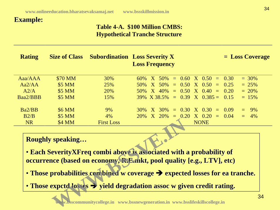
Table 4-A. $100 Million CMBS: Hypothetical Tranche Structure
Rating Size of Class Subordination Loss Severity XLoss Frequency
= Loss Coverage
Aaa/AAA $70 MM 30% 60% X 50% = 0.60 X 0.50 = 0.30 = 30%Aa2/AA $5 MM 25% 50% X 50% = 0.50 X 0.50 = 0.25 = 25%
A2/A $5 MM 20% 50% X 40% = 0.50 X 0.40 = 0.20 = 20%Baa2/BBB $5 MM 15% 39% X 38.5% = 0.39 X 0.385 = 0.15 = 15%
Ba2/BB $6 MM 9% 30% X 30% = 0.30 X 0.30 = 0.09 = 9%B2/B $5 MM 4% 20% X 20% = 0.20 X 0.20 = 0.04 = 4%NR $4 MM First Loss NONE
Example:Example:
Roughly speakingRoughly speaking……
•• Each Each SeverityXFreqSeverityXFreq combicombi above is associated with a probability of above is associated with a probability of occurrence (based on economy, occurrence (based on economy, R.E.mktR.E.mkt, pool quality [e.g., LTV], etc), pool quality [e.g., LTV], etc)
•• Those probabilities combined w coverage Those probabilities combined w coverage expected losses for ea expected losses for ea tranchetranche..
•• Those Those expctdexpctd losses losses yield degradation assoc w given credit rating.yield degradation assoc w given credit rating.
www.bsscommunitycollege.in www.bssnewgeneration.in www.bsslifeskillscollege.in
34www.onlineeducation.bharatsevaksamaj.net www.bssskillmission.in
WWW.BSSVE.IN

35
Historical Commercial Mortgage Defaults
– Esaki, L’Heureux, Snyderman—ELS Study (1999, update in 2002)
– Tracked insurance company commercial mortgage defaults from ’72–’00
– Originated from ’72–’95– Tracked performance through ’00
– Lifetime average default rate was 18%– Highest default rate for any origination cohort was 32% in 1986
– Loss severity averaged 34% on liquidated loans– Approximately 50% defaulted loans liquidated
• Basic formula rating agencies use to figure out credit support:• Default frequency * Loss Severity = Expected Loss
25www.bsscommunitycollege.in www.bssnewgeneration.in www.bsslifeskillscollege.in
35www.onlineeducation.bharatsevaksamaj.net www.bssskillmission.in
WWW.BSSVE.IN

36
Conduit Capital Structurevs. ELS Study
How does the average conduit capital structure compare to the historical commercial mortgage delinquency experience?
Are subordination levels too high? Too low?
Based on the ELS study AAA and AA bonds are sized to withstand a repeat of the late 1980s and not suffer any principal losses
The single A and BBB bonds will not suffer losses under an average stress scenario
• 18% default x 34% loss severity = 6.12% loss
Single As and BBB’s suffer losses based on experience of the worst origination cohort• 32% x 34% = 10.88%
26
17.00%
14.00%
10.50%
6.50%
3.50%
2.00%
0%
AAA(83.00%)
AA(3.00%)
A(3.50%)
BBB(4.00%)
BB(3.00%)
B(1.50%)
UR(2.00%)
% Subordination
Average Default Rate
Worst Cohort (1986)
6.12%
10.88%
www.bsscommunitycollege.in www.bssnewgeneration.in www.bsslifeskillscollege.in
36www.onlineeducation.bharatsevaksamaj.net www.bssskillmission.in
WWW.BSSVE.IN

37
20.3.3 Rating CMBS 20.3.3 Rating CMBS tranchestranches......
CreditCredit--rating agencies employ:rating agencies employ:•• Statistical and analytical techniques,Statistical and analytical techniques,•• Qualitative investigation (Qualitative investigation (incluinclu legal & mgt assessments, due diligence),legal & mgt assessments, due diligence),•• Common sense.Common sense.
The issuerThe issuer’’s track record is considered as well as the pool of loans & the s track record is considered as well as the pool of loans & the underlying property collateral.underlying property collateral.Traditional underwriting measures such as LTV ratio and DCR are Traditional underwriting measures such as LTV ratio and DCR are examined for examined for the pool as a whole. the pool as a whole. Some of the larger mortgages in the pool are examined individualSome of the larger mortgages in the pool are examined individually.ly.Pool Pool aggregateaggregate measures (weighted average) are considered.measures (weighted average) are considered.Pool Pool heterogeneityheterogeneity is also considered:is also considered:
•• Dispersion in LTV & DCR, Dispersion in LTV & DCR, •• Diversification of collateral (by property type, geographic loDiversification of collateral (by property type, geographic location).cation).
Diversity & heterogeneity of the mortgages within a pool can matDiversity & heterogeneity of the mortgages within a pool can matter as much as ter as much as the average characteristics of the pool, esp. for lowerthe average characteristics of the pool, esp. for lower--rated rated tranchestranches::
•• e.g., Diversification e.g., Diversification ReducedReduced default risk for default risk for seniorsenior trances; trances; Increased Increased default risk for default risk for lowerlower tranchestranches (esp. first(esp. first--loss). loss). Why?... Why?...
www.bsscommunitycollege.in www.bssnewgeneration.in www.bsslifeskillscollege.in
37www.onlineeducation.bharatsevaksamaj.net www.bssskillmission.in
WWW.BSSVE.IN

38
20.3.3 Rating CMBS 20.3.3 Rating CMBS tranchestranches (cont.)(cont.)……
•• Overall average LTV ratio & DCROverall average LTV ratio & DCR•• Dispersion (heterogeneity) in LTV and DCRDispersion (heterogeneity) in LTV and DCR•• Quality of LTV and DCR informationQuality of LTV and DCR information•• Property types in the poolProperty types in the pool•• Property ages and lease expirationsProperty ages and lease expirations•• Geographical location of propertiesGeographical location of properties•• Loan sizes & total number of loansLoan sizes & total number of loans•• Loan maturitiesLoan maturities•• Loan terms (e.g., amortization, floating rates, prepayment, Loan terms (e.g., amortization, floating rates, prepayment, recourse)recourse)•• Seasoning (age) of the loansSeasoning (age) of the loans•• Amount of pool Amount of pool overcollatalizationovercollatalization or credit enhancementor credit enhancement•• Legal structure & Legal structure & servicerservicer relationshipsrelationships•• Number of borrowers & crossNumber of borrowers & cross--collateralizationcollateralization
Variables that can be important in analyzing the credit quality Variables that can be important in analyzing the credit quality of a mortgage pool of a mortgage pool and the various and the various tranchestranches that can be carved out of it, in either quantitative or that can be carved out of it, in either quantitative or qualitative analysis, include:qualitative analysis, include:
www.bsscommunitycollege.in www.bssnewgeneration.in www.bsslifeskillscollege.in
38www.onlineeducation.bharatsevaksamaj.net www.bssskillmission.in
WWW.BSSVE.IN

39
20.3.3 Rating CMBS 20.3.3 Rating CMBS tranchestranches (cont.)(cont.)……
Rating agencies (and consultants working for them) employ:Rating agencies (and consultants working for them) employ:
•• Econometric models of commercial mortgage default probability (Econometric models of commercial mortgage default probability (e.g., e.g., logitlogit, , probitprobit binary choice models, proportional hazard models).binary choice models, proportional hazard models).
•• Empirical estimates of conditional loss severity.Empirical estimates of conditional loss severity.
•• Monte Carlo simulation of interest rates, property market, and Monte Carlo simulation of interest rates, property market, and credit credit losses, to losses, to ““stress teststress test”” the pool and the various the pool and the various tranchestranches that may be defined that may be defined based on it.based on it.
Because of the importance of the creditBecause of the importance of the credit--rating function in determining the value rating function in determining the value and hence financial feasibility of a CMBS issue, the and hence financial feasibility of a CMBS issue, the rating agencies play a quasirating agencies play a quasi--regulatory role in the CMBS marketregulatory role in the CMBS market..
(This is much like the role played by FNMA, FHLMC and GNMA as th(This is much like the role played by FNMA, FHLMC and GNMA as the e dominant secondary market buyers and security issuers in the RMBdominant secondary market buyers and security issuers in the RMBS market.) S market.)
The result is greater The result is greater standardizationstandardization of commercial mortgages, especially smaller of commercial mortgages, especially smaller loans of the type that are most likely to be issued by conduits.loans of the type that are most likely to be issued by conduits.
www.bsscommunitycollege.in www.bssnewgeneration.in www.bsslifeskillscollege.in
39www.onlineeducation.bharatsevaksamaj.net www.bssskillmission.in
WWW.BSSVE.IN

40
20.3.4 CMBS Yield Spreads and the Capital Market20.3.4 CMBS Yield Spreads and the Capital Market
Yield spreadsYield spreads reflect the capital marketreflect the capital market’’s evaluation of default risk in CMBS s evaluation of default risk in CMBS tranchestranches. As noted previously, spreads are quoted in two ways, . As noted previously, spreads are quoted in two ways,
““Yield spreadYield spread”” = CMBS yield = CMBS yield –– TT--BondBond yield yield or,or,
““Yield spreadYield spread”” = CMBS yield = CMBS yield –– SwapSwap yieldyield
((where where ““Swap YieldSwap Yield”” is the swapped LIBOR is the swapped LIBOR yldyld, for fixed, for fixed--rate LIBOR of rate LIBOR of same maturity as CMBS WAM.)same maturity as CMBS WAM.)
The Treasury spread can be expressed in terms of the swap spreadThe Treasury spread can be expressed in terms of the swap spread as follows:as follows:
(CMBS (CMBS yldyld –– TT--Bond Bond yldyld) = (CMBS ) = (CMBS yldyld –– Swap Swap yldyld) + (Swap ) + (Swap yldyld –– TT--Bond Bond yldyld))
••Yield spreads can change over time, especially for the higherYield spreads can change over time, especially for the higher--risk risk tranchestranches. .
•• When When mktmkt perceives a threat to credit quality (e.g., recession, overbuilperceives a threat to credit quality (e.g., recession, overbuilding), ding), spreads widen, more so for lowerspreads widen, more so for lower--rated rated tranchestranches (due to greater exposure to (due to greater exposure to default risk and expected magnitude of conditional credit lossesdefault risk and expected magnitude of conditional credit losses). ).
•• A famous and dramatic example of this occurred in 1998 . . .A famous and dramatic example of this occurred in 1998 . . .
1.1. Treasury SpreadTreasury Spread
2.2. Swap SpreadSwap Spread
www.bsscommunitycollege.in www.bssnewgeneration.in www.bsslifeskillscollege.in
40www.onlineeducation.bharatsevaksamaj.net www.bssskillmission.in
WWW.BSSVE.IN

41
Investment Grade CMBS Yields: Spread (basis points) over 10Investment Grade CMBS Yields: Spread (basis points) over 10--yr Treasury Yieldyr Treasury Yield
What happened in 1998??...What happened in 1998??...0
50
100
150
200
250
300
350Fe
b-93
Feb-
94
Feb-
95
Feb-
96
Feb-
97
Feb-
98
Feb-
99
Feb-
00
Feb-
01
Feb-
02
Feb-
03
Feb-
04
Feb-
05
Feb-
06
Source: JP Morgan
Basis Points
AAA AA A BBB
What happened in the fall of 1998?...What happened in the fall of 1998?...
www.bsscommunitycollege.in www.bssnewgeneration.in www.bsslifeskillscollege.in
41www.onlineeducation.bharatsevaksamaj.net www.bssskillmission.in
WWW.BSSVE.IN

42
The 1998 crisis may have been a The 1998 crisis may have been a ““textbook exampletextbook example”” of how the public of how the public capital markets can help to effectively regulate the flow of capcapital markets can help to effectively regulate the flow of capital to the ital to the real estate sector: the real estate sector: the ““negative feedback loopnegative feedback loop”” in the real estate system in the real estate system described in Chapter 2described in Chapter 2……
•• The jump in yields for lowerThe jump in yields for lower--rated CMBS depicted in Exhibit 20rated CMBS depicted in Exhibit 20--10 10 effectively eliminated the market for new issues of CMBS by the effectively eliminated the market for new issues of CMBS by the fall of 1998:fall of 1998:
••Commercial property investors and developers who had been planniCommercial property investors and developers who had been planning to borrow ng to borrow money using the CMBS market as an indirect source of funds (e.g.money using the CMBS market as an indirect source of funds (e.g., through conduit , through conduit mortgages), would have to face interest rates so high, and/or LTmortgages), would have to face interest rates so high, and/or LTV ratio limits so V ratio limits so low, that the financial feasibility of their investments and devlow, that the financial feasibility of their investments and developments would be elopments would be called into question.called into question.••(REIT share prices also tumbled in 1998, temporarily also elimin(REIT share prices also tumbled in 1998, temporarily also eliminating new REIT ating new REIT equity issues as a source of capital for real estate.)equity issues as a source of capital for real estate.)
As a result, the As a result, the flow of capitalflow of capital reaching the real estate sector was cut back. reaching the real estate sector was cut back.
This reduction in capital flow put some breaks on new construcThis reduction in capital flow put some breaks on new construction, directly tion, directly or indirectly resulting in less new space supply coming into theor indirectly resulting in less new space supply coming into the system than system than otherwise would have been the case at that time. otherwise would have been the case at that time.
www.bsscommunitycollege.in www.bssnewgeneration.in www.bsslifeskillscollege.in
42www.onlineeducation.bharatsevaksamaj.net www.bssskillmission.in
WWW.BSSVE.IN

43
A technical result of the 1998 experience is that investment grade CMBS spreads are now typically quoted relative to LIBOR Swaps, rather than Treasury Bonds.
Jan-970
50
100
150
77
4528
200
250
bp
Oct-98 Jun-00 Mar-02 Dec-03 Sep-05
10-Year Swap SpreadsAAA CMBS to USTAAA CMBS to Swaps
10-Year AAA Spreads
Figure by MIT OCW, adapted from course textbook.www.bsscommunitycollege.in www.bssnewgeneration.in www.bsslifeskillscollege.in
43www.onlineeducation.bharatsevaksamaj.net www.bssskillmission.in
WWW.BSSVE.IN

44
Swap spreads reflect credit risk in fixed income-markets in general, that is not real estate specific. The CMBS spread to the fixed swap rate then adds the incremental risks specific to CMBS; the CMBS spread above Tsy reflects both.
LIBOR Swaps contain a little bit of default riskdefault risk (more than T-Bonds, Less than CMBS AAA), but ““liquidity riskliquidity risk”” similar to CMBS AAA tranche.
=> Swap spreads tend to be highly correlated with CMBS spreads, and as a result CMBS players use swaps to hedge when accumulating loans to securitize.
CMBS Spreads to Treasuryand Swap Benchmarks(example numbers as oflate 2005)
CMBSSpreadto Swaps= 35 bp
SwapSpreadto TSY= 40 bp
CMBS Yield Spreadto Treasuries (TSY)= 75 bp
10-Year AAA CMBS Yield
10-Year Swap Yield
10-Year Treasury Yield
5.25%
4.90%
4.5%
Figure by MIT OCW, adapted from course textbook.
www.bsscommunitycollege.in www.bssnewgeneration.in www.bsslifeskillscollege.in
44www.onlineeducation.bharatsevaksamaj.net www.bssskillmission.in
WWW.BSSVE.IN

45
The difference is not so much a perception of greater default risk per se, but greater “liquidity risk”(difficulty selling securities at full value during “events”, times of shock or crisis in the financial markets), even though the underlying credit quality of the pool may be relatively unaffected.
(Of course, default risk must underlie this type of liquidity risk at a deeper level, because U.S. T-Bonds do not suffer from liquidity risk, presumably because they are free of any default risk, so investors feel confident pricing them even during financial crises. This is also facilitated by the depth and breadth of the T-Bond market, the sheer quantity of homogeneous securities issued. For both these reasons, T-Bonds are the recipient of a “flight to quality”.)
120
100
80
60
40
20
0Jan-97 Sep-98 Jun-00 Mar-02 Dec-03 Sep-05
PreshockingTradingRange
LTCM Shock & Aftermath
Post 9/11
Trading Range since 10/11/03
47373227
22Post ShockTrading Range
bpAAA Spreads to Swap
Figure by MIT OCW, adapted from course textbook.
www.bsscommunitycollege.in www.bssnewgeneration.in www.bsslifeskillscollege.in
45www.onlineeducation.bharatsevaksamaj.net www.bssskillmission.in
WWW.BSSVE.IN

46
The 1998 experience was a major event in the process of the CMBSThe 1998 experience was a major event in the process of the CMBS market market maturing and maturing and ““cutting its teethcutting its teeth””, the first major crisis faced by the market., the first major crisis faced by the market.Yield spreads seem to have made a permanent (?) adjustment sinceYield spreads seem to have made a permanent (?) adjustment since thenthen……
700
290
Non-Investment Grade Spreads to Treasuries
0
200
400
600
800
1000
1200
bp
Jan-98 Jul-99 Feb-01 Aug-02 Mar-04 Sep-05
B 10-Year
BB 10-Year110
564632
Investment Grade Spreads to Swaps
0
50
100
150
200
250
300
bp
Dec-93 May-96 Sep-98 Jan-01 May-03 Sep-05
BBBAAAAAA
Figure by MIT OCW, adapted from course textbook.
www.bsscommunitycollege.in www.bssnewgeneration.in www.bsslifeskillscollege.in
46www.onlineeducation.bharatsevaksamaj.net www.bssskillmission.in
WWW.BSSVE.IN

47
CMBS Mkt Yld Spreads over 10-yr T-BondsDec.2004 Dec.1998 Apr-98
AAA 70 136 77AA 77 161 88A 85 186 105BBB 127 275 140BB 325 575 250B 770 825 450
Spreads have recently come down to below preSpreads have recently come down to below pre--crisis (of 98) levelscrisis (of 98) levels……
www.bsscommunitycollege.in www.bssnewgeneration.in www.bsslifeskillscollege.in
47www.onlineeducation.bharatsevaksamaj.net www.bssskillmission.in
WWW.BSSVE.IN

48
Credit support levels…too high, too low, just right?
1996 1997 1998 1999 2000 2001 2002 2003 2004
AAA 31.5 30.3 28.8 27.0 22.2 21.0 20.7 16.5 13.7
AA 25.3 24.1 23.7 22.3 17.8 17.4 16.1 13.7 11.1
A 19.7 18.5 18.7 17.3 13.7 12.9 12.3 10.0 8.1
BBB 14.8 13.3 12.6 12.3 9.6 9.1 8.1 6.7 4.9
BBB- 12.6 11.5 10.9 10.5 8.3 7.6 7.2 5.2 3.6
BB 7.9 6.0 5.8 6.1 4.5 4.6 4.4 3.5 2.7
B 3.3 3.0 3.2 2.9 2.1 2.4 2.2 1.9 1.6
Weighted-average fixed-rate conduit CMBS subordination (%)Weighted-average fixed-rate conduit CMBS subordination (%)
Source: JPMorgan Research
Subordination levels have fallen steadily since the late 1990s and took another sharp drop in 2004. How low can they go?
However, we have probably hit a plateau for a short while given the “frothiness” of the current lending environment
7CR
ED
IT
SU
PP
OR
TL
EV
EL
S
www.bsscommunitycollege.in www.bssnewgeneration.in www.bsslifeskillscollege.in
48www.onlineeducation.bharatsevaksamaj.net www.bssskillmission.in
WWW.BSSVE.IN

49
CMBS CMBS vsvs Corporate Corporate Bond Market Yield Bond Market Yield Spreads in Spreads in Comparable Comparable Maturity Maturity AA--rated rated Securities:Securities:
20.3.5 CMBS versus corporate bond spreads20.3.5 CMBS versus corporate bond spreads
Throughout much of their early history, CMBS yields generally exThroughout much of their early history, CMBS yields generally exceeded those on ceeded those on similar maturity corporate bonds of equal credit rating.similar maturity corporate bonds of equal credit rating.
Why would this be?...Why would this be?...
-50
0
50
100
150
200
250
300
Jan-
96
Jul-9
6
Jan-
97
Jul-9
7
Jan-
98
Jul-9
8
Jan-
99
Jul-9
9
Jan-
00
Jul-0
0
Jan-
01
Jul-0
1
Jan-
02
Jul-0
2
Jan-
03
Jul-0
3
Jan-
04
Jul-0
4
Jan-
05
Jul-0
5
Jan-
06
Jul-0
6
Source: JP Morgan and Lehman
Basis Points
CMBS Corporate Difference
www.bsscommunitycollege.in www.bssnewgeneration.in www.bsslifeskillscollege.in
49www.onlineeducation.bharatsevaksamaj.net www.bssskillmission.in
WWW.BSSVE.IN

50
CMBS are CMBS are ““different animalsdifferent animals”” compared to corporate bonds:compared to corporate bonds:1.1. Prepayment Risk:Prepayment Risk: Most U.S. commercial mortgs have “prepayment protection”, but some do not
(or it is imperfect, or goes away). Some CMBS pools contain mortgages that are more like callable corporate bonds, resulting in a yield premium to reflect the prepayment risk faced by the investor. Such a yield premium would affect spreads for all tranches, but especially for senior tranches, given the typical principal payback priority structure.
2.2. Agency and Extension Risk:Agency and Extension Risk: In the event of default in CMBS pools, a conflict of interest tends to exist between investors in senior versus junior tranches. The former want immediate foreclosure, while the latter tend to prefer a workout and extension of loan term. The authority to decide whether to foreclose or exercise forebearance is vested in the “special servicer”, who is usually effectively controlled by the junior tranche holders (after all, they stand to lose or gain the most from how the default is handled). Foreclosure/workout decision cannot be expected to be handled optimally from the senior tranche holders’ perspective. Higher yield in the senior tranches. No such conflict of interest exists in typical corporate bonds because there is only one class of investor.
3.3. Credit Information Quality and GoingCredit Information Quality and Going--concern Risk & Liquidity Implications:concern Risk & Liquidity Implications: Bonds backed by large publicly-traded corporations have available more on-going information relevant to the credit risk of the borrower. Also, the public corporation is a single going-concern that typically knows it will need to return to the bond market again, probably regularly in the near and long-term future. It therefore must carefully consider its reputation in the bond market, and this makes it less likely to default on its bonds. Rating agencies and investors were initially more “in the dark” about the credit risk of the typical CMBS issue than they are with the typical corporate bond. This concern was (still is?) especially relevant for the lower-rated tranches.
20.3.5 CMBS versus corporate bond spreads20.3.5 CMBS versus corporate bond spreads
www.bsscommunitycollege.in www.bssnewgeneration.in www.bsslifeskillscollege.in
50www.onlineeducation.bharatsevaksamaj.net www.bssskillmission.in
WWW.BSSVE.IN

51
• Such differences as these between CMBS and corporate bonds presumably explain the difference in yields for otherwise similar maturity bonds with the same credit-rating.
• The higher CMBS spreads cannot be presumed to give CMBS investors “something for nothing”, that is, a better risk-adjusted expected return than corporate bonds.
• Also, CMBS were still a new type of security in the 1990s. The capital markets were still learning about the nature of their risk and return. The CMBS industry seems to be evolving toward the mitigation of some of the differences noted here, esp. for more senior tranches. There is mounting evidence that the spread between CMBS and equivalent corporate bonds has been recently narrowing…
20.3.5 CMBS versus corporate bond spreads20.3.5 CMBS versus corporate bond spreads
History seems to be proving the 3rd bullet point true.
www.bsscommunitycollege.in www.bssnewgeneration.in www.bsslifeskillscollege.in
51www.onlineeducation.bharatsevaksamaj.net www.bssskillmission.in
WWW.BSSVE.IN

52
–Historically BBB CMBS has traded wide (cheap) to BBB corporates
– In 2003-04 BBB CMBS traded on top of BBB corporates
Since 2002 there has beenSince 2002 there has been very little spread between very little spread between CMBSCMBS and C and Coorporate I.G. rporate I.G.
yields.yields.
Jan-97 Oct-98 Jun-00 Mar-02 Dec-03 Sep-05
350
300
250
200
150
100
50
0
-50
bp 155
123
32
BBB CMBS to USTBBB Corporate Industrials Spreads to USTDifference
Source: Morgan Stanley.
10-Year BBB CMBS Spread versus BBB Corporate Industrial Spreads to Treasuries
Figure by MIT OCW, adapted from course textbook.www.bsscommunitycollege.in www.bssnewgeneration.in www.bsslifeskillscollege.in
52www.onlineeducation.bharatsevaksamaj.net www.bssskillmission.in
WWW.BSSVE.IN
53
20.4 CMBS Borrower Considerations20.4 CMBS Borrower Considerations•• Borrowers must understand that REMIC Borrowers must understand that REMIC regulations limit the ability of regulations limit the ability of servicersservicers to to change mortgage loan documents once a loan is change mortgage loan documents once a loan is securitized securitized ……
→→ CMBS is a relatively inflexible; postCMBS is a relatively inflexible; post--loan loan closing, it is difficult to modify the collateral closing, it is difficult to modify the collateral (i.e. property), (i.e. property), unless planned for and included unless planned for and included in the loan documents at the time of closing.in the loan documents at the time of closing.
→→ CMBS loans are generally not well suited for CMBS loans are generally not well suited for properties with significant expansion properties with significant expansion possibilities and/or redevelopment potential.possibilities and/or redevelopment potential.
•• CMBS provides relatively standardized, CMBS provides relatively standardized, cookiecookie--cutter loans.cutter loans.
→→ Not for borrowers looking for a customized Not for borrowers looking for a customized loan or relationshiploan or relationship--based lending based lending
www.bsscommunitycollege.in www.bssnewgeneration.in www.bsslifeskillscollege.in
53www.onlineeducation.bharatsevaksamaj.net www.bssskillmission.in
WWW.BSSVE.IN

54
Ch.20 CMBS Summary;Ch.20 CMBS Summary;
•• CMBS have unique investment characteristics (relatively little CMBS have unique investment characteristics (relatively little prepayment risk, prepayment risk, relatively high yields) that appeal to important classes of inverelatively high yields) that appeal to important classes of investors, thereby increasing stors, thereby increasing the capital available to real estate, and improving the efficienthe capital available to real estate, and improving the efficiency of the functioning of cy of the functioning of the capital market for investors.the capital market for investors.
•• Variety in the risk and return attributes of the securities carVariety in the risk and return attributes of the securities carved out of a mortgage ved out of a mortgage pool allow different pool allow different tranchestranches to appeal to different types of investors. to appeal to different types of investors.
•• The CMBS market is another example of how investor heterogeneitThe CMBS market is another example of how investor heterogeneity drives the y drives the investment industry. investment industry.
•• Typically, the Typically, the investmentinvestment--grade grade tranchestranches that make up the bulk of a typical CMBS that make up the bulk of a typical CMBS issue find ready buyers in the form of conservative institutionsissue find ready buyers in the form of conservative institutions such as such as pension fundspension funds, , life insurance companieslife insurance companies, and , and bond mutual fundsbond mutual funds. .
•• The market for the more risky speculative and junk The market for the more risky speculative and junk tranchestranches is much thinner. is much thinner.
•• Major buyers and holders of the lower Major buyers and holders of the lower tranchestranches are aggressive investors willing to are aggressive investors willing to take on risk for high expected returns, and who typically have stake on risk for high expected returns, and who typically have specialized knowledge pecialized knowledge and expertise regarding commercial property risk. and expertise regarding commercial property risk.
•• Such investors have included the Such investors have included the investment banksinvestment banks and and conduits issuingconduits issuing the CMBS, the CMBS, the the ““special special servicersservicers”” who are charged with taking over defaulted loans in the pool towho are charged with taking over defaulted loans in the pool toattempt attempt ““workoutsworkouts”” with the borrowers, and specialized with the borrowers, and specialized mortgage mortgage REITsREITs ..
www.bsscommunitycollege.in www.bssnewgeneration.in www.bsslifeskillscollege.in
54www.onlineeducation.bharatsevaksamaj.net www.bssskillmission.in
WWW.BSSVE.IN

1
Chapter 21 Chapter 21
Modern Portfolio TheoryModern Portfolio Theory
& &
Chapter 22Chapter 22
Equilibrium Asset PricingEquilibrium Asset Pricing
www.bsscommunitycollege.in www.bssnewgeneration.in www.bsslifeskillscollege.in
55www.onlineeducation.bharatsevaksamaj.net www.bssskillmission.in
WWW.BSSVE.IN

2
"MODERN PORTFOLIO THEORY"
(aka "Mean-Variance Portfolio Theory", or “Markowitz Portfolio Theory” – Either way: “MPT” for short)
DEVELOPED IN 1950s (by MARKOWITZ, SHARPE, LINTNER)
(Won Nobel Prize in Economics in 1990.)
WIDELY USED AMONG PROFESSIONAL INVESTORS
FUNDAMENTAL DISCIPLINE OF PORTFOLIO-LEVEL INVESTMENT STRATEGIC DECISION MAKING.
21.2 Basic Mean-Variance Portfolio Theory
www.bsscommunitycollege.in www.bssnewgeneration.in www.bsslifeskillscollege.in
56www.onlineeducation.bharatsevaksamaj.net www.bssskillmission.in
WWW.BSSVE.IN

3
I. REVIEW OF STATISTICS ABOUT PERIODIC TOTAL RETURNS: (Note: these are all “time-series” statistics: measured across time, not across assets within a single point in time.) "1st Moment" Across Time (measures “central tendency”): “MEAN”, used to measure: Expected Performance ("ex ante", usually arithmetic mean: used in portf ana.) Achieved Performance ("ex post", usually geometric mean) "2nd Moments" Across Time (measure characteristics of the deviation around the central tendancy). They include… 1) "STANDARD DEVIATION" (aka "volatility"), which measures:
Square root of variance of returns across time. "Total Risk" (of exposure to asset if investor not diversified)
2) "COVARIANCE", which measures "Co-Movement", aka:
"Systematic Risk" (component of total risk which cannot be "diversified away") Covariance with investor’s portfolio measures asset contribution to portfolio total
risk. 3) "CROSS-CORRELATION" (just “correlation” for short). Based on contemporaneous covariance between two assets or asset classes. Measures how two assets "move together": important for Portfolio Analysis. 4) "AUTOCORRELATION" (or “serial correlation”: Correlation with itself across time), which reflects the nature of the "Informational Efficiency" in the Asset Market; e.g.: Zero "Efficient" Market (prices quickly reflect full information; returns
lack predictability) Like securities markets (approximately).
Positive "Sluggish" (inertia, inefficient) Market (prices only gradually incorporate new info.) Like private real estate markets.
Negative "Noisy" Mkt (excessive s.r. volatility, price "overreactions") Like securities markets (to some extent).
See Chapter Appendix
www.bsscommunitycollege.in www.bssnewgeneration.in www.bsslifeskillscollege.in
57www.onlineeducation.bharatsevaksamaj.net www.bssskillmission.in
WWW.BSSVE.IN

4
"Picture" of 1st and 2nd Moments . . .
First Moment is "Trend“. Second Moment is "Deviation" around trend.Food for Thought Question:IF THE TWO LINES ABOVE WERE TWO DIFFERENT ASSETS, WHICH WOULD YOU PREFER TO INVEST IN, OTHER THINGS BEING EQUAL? . . .
30
25
20
15
10
5
01977 2002 2027 2052 2077 2102 2127 2152 2177 2202 2227
Ass
et V
alue
Actual Asset Value1st & 2nd Moment of Return
L.R. Trend Asset Value1st Moment Only of Return
Year
Figure by MIT OCW.
www.bsscommunitycollege.in www.bssnewgeneration.in www.bsslifeskillscollege.in
58www.onlineeducation.bharatsevaksamaj.net www.bssskillmission.in
WWW.BSSVE.IN

5
S&P500S&P500 LTG BondsLTG Bonds Private Real Private Real EstateEstate
Mean (Mean (aritharith)) 12.7%12.7% 9.7%9.7% 9.9%9.9%
Std.DeviationStd.Deviation 17.5%17.5% 11.8%11.8% 9.0%9.0%
Correlations:Correlations:
S&P500S&P500 100%100% 27.2%27.2% 16.6%16.6%
LTG BondsLTG Bonds 100%100% --21.0%21.0%
PrivPriv. Real Estate. Real Estate 100%100%
Historical statistics, annual periodic total returns: Historical statistics, annual periodic total returns: Stocks, Bonds, Real Estate, 1970Stocks, Bonds, Real Estate, 1970--20032003……
PORTFOLIO THEORY IS A WAY TO CONSIDER PORTFOLIO THEORY IS A WAY TO CONSIDER BOTHBOTH THE THE 1ST1ST & & 2ND2ND MOMENTS (& INTEGRATE THE TWO) IN INVESTMENT MOMENTS (& INTEGRATE THE TWO) IN INVESTMENT ANALYSIS.ANALYSIS.
11stst MomentsMoments
22ndnd MomentsMoments
www.bsscommunitycollege.in www.bssnewgeneration.in www.bsslifeskillscollege.in
59www.onlineeducation.bharatsevaksamaj.net www.bssskillmission.in
WWW.BSSVE.IN

6
21.2.1.21.2.1. Investor Preferences & Dominant PortfoliosInvestor Preferences & Dominant Portfolios
SUPPOSE WE DRAW A 2SUPPOSE WE DRAW A 2--DIMENSIONAL SPACE WITH RISK (2NDDIMENSIONAL SPACE WITH RISK (2ND--MOMENT) MOMENT) ON HORIZONTAL AXIS AND EXPECTED RETURN (1ST MOMENT) ON ON HORIZONTAL AXIS AND EXPECTED RETURN (1ST MOMENT) ON VERTICAL AXIS.VERTICAL AXIS.
A RISKA RISK--AVERSE INVESTOR MIGHT HAVE A UTILITY (PREFERENCE) AVERSE INVESTOR MIGHT HAVE A UTILITY (PREFERENCE) SURFACE INDICATED BY CONTOUR LINES LIKE THESE (investor is indifSURFACE INDICATED BY CONTOUR LINES LIKE THESE (investor is indifferent ferent along a given contour line):along a given contour line):
RISKRISK
RETURNRETURNP
Q
THE CONTOUR LINES ARE STEEPLY RISING AS THE RISKTHE CONTOUR LINES ARE STEEPLY RISING AS THE RISK--AVERSE AVERSE INVESTOR WANTS MUCH MORE RETURN TO COMPENSATE FOR A LITTLE INVESTOR WANTS MUCH MORE RETURN TO COMPENSATE FOR A LITTLE MORE RISK.MORE RISK.
www.bsscommunitycollege.in www.bssnewgeneration.in www.bsslifeskillscollege.in
60www.onlineeducation.bharatsevaksamaj.net www.bssskillmission.in
WWW.BSSVE.IN

7
A MORE AGGRESSIVE INVESTOR MIGHT HAVE A UTILITY A MORE AGGRESSIVE INVESTOR MIGHT HAVE A UTILITY (PREFERENCE) SURFACE INDICATED BY CONTOUR LINES LIKE THESE.(PREFERENCE) SURFACE INDICATED BY CONTOUR LINES LIKE THESE.
RISKRISK
RETURNRETURNP
Q
THE SHALLOW CONTOUR LINES INDICATE THE INVESTOR DOES NOT THE SHALLOW CONTOUR LINES INDICATE THE INVESTOR DOES NOT NEED MUCH ADDITIONAL RETURN TO COMPENSATE FOR MORE RISK.NEED MUCH ADDITIONAL RETURN TO COMPENSATE FOR MORE RISK.
BUT BOTH INVESTORS WOULD AGREE THEY PREFER POINTS TO BUT BOTH INVESTORS WOULD AGREE THEY PREFER POINTS TO THE "NORTH" AND "WEST" IN THE RISK/RETURN SPACE. THEY THE "NORTH" AND "WEST" IN THE RISK/RETURN SPACE. THEY BOTH PREFER POINT "P" TO POINT "Q".BOTH PREFER POINT "P" TO POINT "Q".
www.bsscommunitycollege.in www.bssnewgeneration.in www.bsslifeskillscollege.in
61www.onlineeducation.bharatsevaksamaj.net www.bssskillmission.in
WWW.BSSVE.IN

8
FOR ANY TWO PORTFOLIOS "P" AND "Q" SUCH THAT:FOR ANY TWO PORTFOLIOS "P" AND "Q" SUCH THAT:EXPECTED RETURN "P" EXPECTED RETURN "P" ≥≥ EXPECTED RETURN "Q"EXPECTED RETURN "Q"
AND (SIMULTANEOUSLY): AND (SIMULTANEOUSLY): RISK "P" RISK "P" ≤≤ RISK "Q"RISK "Q"IT IS SAID THAT: IT IS SAID THAT: ““QQ”” IS IS DOMINATEDDOMINATED BY BY ““PP””..
THIS IS INDEPENDENT OF RISK PREFERENCES. THIS IS INDEPENDENT OF RISK PREFERENCES. BOTH CONSERVATIVE AND AGGRESSIVE INVESTORS WOULD BOTH CONSERVATIVE AND AGGRESSIVE INVESTORS WOULD
AGREE ABOUT THIS.AGREE ABOUT THIS.
IN ESSENCE, PORTFOLIO THEORY IS ABOUT HOW TO AVOID INVESTING IN ESSENCE, PORTFOLIO THEORY IS ABOUT HOW TO AVOID INVESTING IN DOMINATED PORTFOLIOS.IN DOMINATED PORTFOLIOS.
RISKRISK
RETURNRETURNP
QDOMINATED
BY"Q"
DOMINATES"Q"
PORTFOLIO THEORY TRIES TO MOVE INVESTORS PORTFOLIO THEORY TRIES TO MOVE INVESTORS FROM POINTS LIKE "Q" TO POINTS LIKE "P".FROM POINTS LIKE "Q" TO POINTS LIKE "P".
DOMINATES"Q"
www.bsscommunitycollege.in www.bssnewgeneration.in www.bsslifeskillscollege.in
62www.onlineeducation.bharatsevaksamaj.net www.bssskillmission.in
WWW.BSSVE.IN

9
III. PORTFOLIO THEORY AND DIVERSIFICATION... "PORTFOLIOS" ARE "COMBINATIONS OF ASSETS".
In other words, GIVEN YOUR OVERALL INVESTABLE WEALTH, PORTFOLIO THEORY TELLS YOU HOW MUCH YOU SHOULD INVEST IN DIFFERENT TYPES OF ASSETS. FOR EXAMPLE: WHAT % SHOULD YOU PUT IN REAL ESTATE? WHAT % SHOULD YOU PUT IN STOCKS? TO BEGIN TO RIGOROUSLY ANSWER THIS QUESTION, CONSIDER...
PORTFOLIO THEORY FOR (or from) YOUR GRANDMOTHER:
“DON’T PUT ALL YOUR EGGS IN ONE BASKET!” WHAT MORE THAN THIS CAN WE SAY? . . .
(e.g., How many “eggs” should we put in which “baskets”.)
Section 21.2.2Section 21.2.2……
www.bsscommunitycollege.in www.bssnewgeneration.in www.bsslifeskillscollege.in
63www.onlineeducation.bharatsevaksamaj.net www.bssskillmission.in
WWW.BSSVE.IN

10
AT THE HEART OF PORTFOLIO THEORY ARE TWO BASIC AT THE HEART OF PORTFOLIO THEORY ARE TWO BASIC MATHEMATICAL MATHEMATICAL FACTSFACTS::
1) PORTFOLIO RETURN IS A LINEAR FUNCTION OF THE ASSET 1) PORTFOLIO RETURN IS A LINEAR FUNCTION OF THE ASSET WEIGHTS:WEIGHTS:
IN PARTICULAR, THE PORTFOLIO EXPECTED RETURN IS A IN PARTICULAR, THE PORTFOLIO EXPECTED RETURN IS A WEIGHTED AVERAGEWEIGHTED AVERAGE OF THE EXPECTED RETURNS TO THE OF THE EXPECTED RETURNS TO THE INDIVIDUAL ASSETS. E.G., WITH TWO ASSETS ("i" & "j"):INDIVIDUAL ASSETS. E.G., WITH TWO ASSETS ("i" & "j"):
rrpp = = ωωrrii + (1+ (1--ωω))rrjj
WHERE WHERE ωωii IS THE SHARE OF PORTFOLIO TOTAL VALUE INVESTED IS THE SHARE OF PORTFOLIO TOTAL VALUE INVESTED IN ASSET i.IN ASSET i.
e.g., If Asset A has E[rA]=5% and Asset B has E[rB]=10%, then a 50/50 Portfolio (50% A + 50% B) will have E[rP]=7.5%.
rw=r nn
N
1=nP ∑
www.bsscommunitycollege.in www.bssnewgeneration.in www.bsslifeskillscollege.in
64www.onlineeducation.bharatsevaksamaj.net www.bssskillmission.in
WWW.BSSVE.IN

11
2) PORTFOLIO VOLATILITY IS A NON2) PORTFOLIO VOLATILITY IS A NON--LINEAR FUNCTION OF THE LINEAR FUNCTION OF THE ASSET WEIGHTS:ASSET WEIGHTS:
SUCH THAT THE PORTFOLIO VOLATILITY IS SUCH THAT THE PORTFOLIO VOLATILITY IS LESS THANLESS THAN A A WEIGHTED AVERAGE OF THE VOLATILITIES OF THE WEIGHTED AVERAGE OF THE VOLATILITIES OF THE INDIVIDUAL ASSETS. E.G., WITH TWO ASSETS:INDIVIDUAL ASSETS. E.G., WITH TWO ASSETS:
This is the beauty of Diversification. It is at the core of Portfolio Theory. It is perhaps the only place in economics where you get a “free lunch”: In this case, less risk without necessarily reducing your expected return!
e.g., If Asset A has StdDev[rA]=5% and Asset B has StdDev[rB]=10%, then a 50/50 Portfolio (50% A + 50% B) will have StdDev[rP] < 7.5% (conceivably even < 5%).
THE 2THE 2NDND FACT:FACT:
ssPP = = √√[ [ ωω²²(s(sii))²² + (1+ (1--ωω))²²(s(sjj))²² + 2+ 2ωω(1(1--ωω)s)siissjjCCij ij ] ]
≤≤ ωωssii + (1+ (1--ωω)s)sjj
WHERE WHERE ssii IS THE RISK (MEASURED BY STD.DEV.) OF ASSET i.IS THE RISK (MEASURED BY STD.DEV.) OF ASSET i.
∑∑= =
=N
I
N
JijjiP COVwwVAR
1 1
www.bsscommunitycollege.in www.bssnewgeneration.in www.bsslifeskillscollege.in
65www.onlineeducation.bharatsevaksamaj.net www.bssskillmission.in
WWW.BSSVE.IN

12
Stocks & bonds (+30% correlation): Each dot is one year's returns.
Stock & Bond Ann. Returns, 1970-2003: +30% Correlation
-20%
-10%
0%
10%
20%
30%
40%
50%
-30% -20% -10% 0% 10% 20% 30% 40% 50%
Stock Returns
Bon
d R
etur
ns
The diversification effect is greater the less correlated are the assets…
www.bsscommunitycollege.in www.bssnewgeneration.in www.bsslifeskillscollege.in
66www.onlineeducation.bharatsevaksamaj.net www.bssskillmission.in
WWW.BSSVE.IN

13
Stocks & real estate (+17% correlation): Each dot is one year's returns.
Real Est. & Stock Ann. Returns, 1970-2003: +17% Correlation
-15%
-10%
-5%
0%
5%
10%
15%
20%
25%
30%
-30% -20% -10% 0% 10% 20% 30% 40% 50%
Stock Returns
R.E
. Ret
urns
The diversification effect is greater the less correlated are the assets…
www.bsscommunitycollege.in www.bssnewgeneration.in www.bsslifeskillscollege.in
67www.onlineeducation.bharatsevaksamaj.net www.bssskillmission.in
WWW.BSSVE.IN
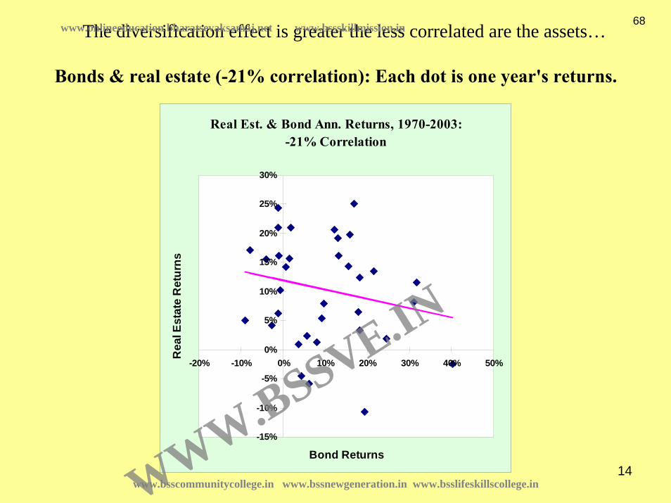
14
Bonds & real estate (-21% correlation): Each dot is one year's returns.
Real Est. & Bond Ann. Returns, 1970-2003: -21% Correlation
-15%
-10%
-5%
0%
5%
10%
15%
20%
25%
30%
-20% -10% 0% 10% 20% 30% 40% 50%
Bond Returns
Rea
l Est
ate
Ret
urns
The diversification effect is greater the less correlated are the assets…
www.bsscommunitycollege.in www.bssnewgeneration.in www.bsslifeskillscollege.in
68www.onlineeducation.bharatsevaksamaj.net www.bssskillmission.in
WWW.BSSVE.IN
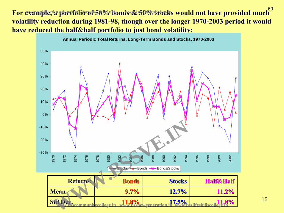
15
For example, a portfolio of 50% bonds & 50% stocks would not havFor example, a portfolio of 50% bonds & 50% stocks would not have provided much e provided much volatility reduction during 1981volatility reduction during 1981--98, though over the longer 197098, though over the longer 1970--2003 period it would 2003 period it would have reduced the have reduced the half&halfhalf&half portfolio to just bond volatility:portfolio to just bond volatility:
Returns:Returns: BondsBonds StocksStocks Half&HalfHalf&Half
MeanMean 9.7%9.7% 12.7%12.7% 11.2%11.2%
Std.DevStd.Dev.. 11.8%11.8% 17.5%17.5% 11.8%11.8%
Annual Periodic Total Returns, Long-Term Bonds and Stocks, 1970-2003
-30%
-20%
-10%
0%
10%
20%
30%
40%
50%19
70
1972
1974
1976
1978
1980
1982
1984
1986
1988
1990
1992
1994
1996
1998
2000
2002
Stocks Bonds Bonds/Stocks
www.bsscommunitycollege.in www.bssnewgeneration.in www.bsslifeskillscollege.in
69www.onlineeducation.bharatsevaksamaj.net www.bssskillmission.in
WWW.BSSVE.IN

16
Here the portfolio of 50% bonds & 50% real estate would have proHere the portfolio of 50% bonds & 50% real estate would have provided a more vided a more consistent diversification during 1970consistent diversification during 1970--2003, with less volatility than either asset class 2003, with less volatility than either asset class alone even though a very similar return:alone even though a very similar return:
Returns:Returns: BondsBonds R.EstateR.Estate Half&HalfHalf&Half
MeanMean 9.7%9.7% 9.9%9.9% 9.8%9.8%
Std.DevStd.Dev.. 11.8%11.8% 9.0%9.0% 6.6%6.6%
Annual Periodic Total Returns, Long-Term Bonds and Real Estate, 1970-2003
-30%
-20%
-10%
0%
10%
20%
30%
40%
50%19
70
1972
1974
1976
1978
1980
1982
1984
1986
1988
1990
1992
1994
1996
1998
2000
2002
Real Estate Bonds Bonds/Real Estate
www.bsscommunitycollege.in www.bssnewgeneration.in www.bsslifeskillscollege.in
70www.onlineeducation.bharatsevaksamaj.net www.bssskillmission.in
WWW.BSSVE.IN

17
This This ““Diversification EffectDiversification Effect”” is greater, the lower is the correlation among the is greater, the lower is the correlation among the assets in the portfolio.assets in the portfolio.
NUMERICAL EXAMPLE . . . SUPPOSE REAL ESTATE HAS: SUPPOSE STOCKS HAVE: EXPECTED RETURN = 8% EXPECTED RETURN = 12% RISK (STD.DEV) = 10% RISK (STD.DEV) = 15% THEN A PORTFOLIO WITH ω SHARE IN REAL ESTATE & (1-ω) SHARE IN STOCKS WILL RESULT IN THESE RISK/RETURN COMBINATIONS, DEPENDING ON THE CORRELATION BETWEEN THE REAL ESTATE AND STOCK RETURNS:
C = 100% C = 25% C = 0% C = -50% ω rP sP rP sP rP sP rP sP 0% 12.0% 15.0% 12.0% 15.0% 12.0% 15.0% 12.0% 15.0%25% 11.0% 13.8% 11.0% 12.1% 11.0% 11.5% 11.0% 10.2%50% 10.0% 12.5% 10.0% 10.0% 10.0% 9.0% 10.0% 6.6%75% 9.0% 11.3% 9.0% 9.2% 9.0% 8.4% 9.0% 6.5%100% 8.0% 10.0% 8.0% 10.0% 8.0% 10.0% 8.0% 10.0%where: C = Correlation Coefficient between Stocks & Real Estate. (This table was simply computed using the formulas noted previously.)
www.bsscommunitycollege.in www.bssnewgeneration.in www.bsslifeskillscollege.in
71www.onlineeducation.bharatsevaksamaj.net www.bssskillmission.in
WWW.BSSVE.IN
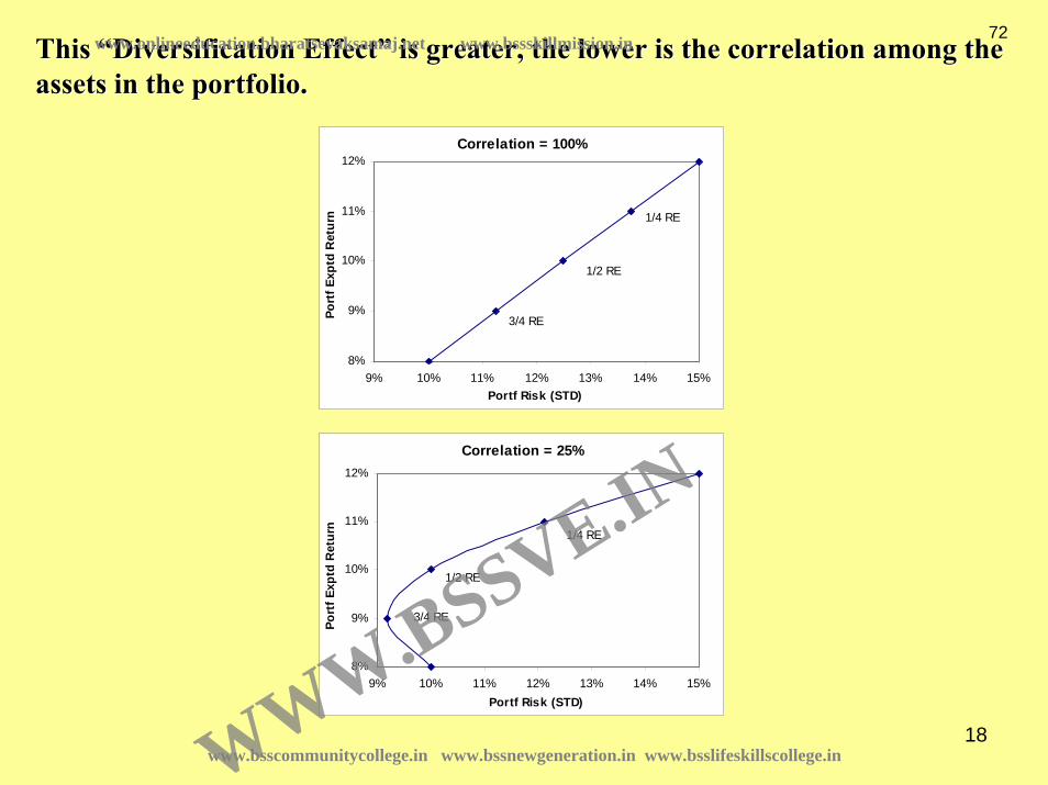
18
Correlation = 100%
8%
9%
10%
11%
12%
9% 10% 11% 12% 13% 14% 15%Portf Risk (STD)
Port
f Exp
td R
etur
n3/4 RE
1/2 RE
1/4 RE
Correlation = 25%
8%
9%
10%
11%
12%
9% 10% 11% 12% 13% 14% 15%Portf Risk (STD)
Port
f Exp
td R
etur
n
1/4 RE
1/2 RE
3/4 RE
This This ““Diversification EffectDiversification Effect”” is greater, the lower is the correlation among the is greater, the lower is the correlation among the assets in the portfolio.assets in the portfolio.
www.bsscommunitycollege.in www.bssnewgeneration.in www.bsslifeskillscollege.in
72www.onlineeducation.bharatsevaksamaj.net www.bssskillmission.in
WWW.BSSVE.IN

19
IN ESSENCE,IN ESSENCE,
PORTFOLIO THEORY PORTFOLIO THEORY ASSUMESASSUMES::
YOUR YOUR OBJECTIVEOBJECTIVE FOR YOUR FOR YOUR OVERALL WEALTHOVERALL WEALTHPORTFOLIO IS:PORTFOLIO IS:
MAXIMIZE EXPECTED FUTURE RETURNMAXIMIZE EXPECTED FUTURE RETURN
MINIMIZE RISK IN THE FUTURE RETURNMINIMIZE RISK IN THE FUTURE RETURN
GIVEN THIS BASIC ASSUMPTION, AND THE EFFECT OF GIVEN THIS BASIC ASSUMPTION, AND THE EFFECT OF DIVERSIFICATION, WE ARRIVE AT THE FIRST MAJOR DIVERSIFICATION, WE ARRIVE AT THE FIRST MAJOR RESULT OF PORTFOLIO THEORY. . .RESULT OF PORTFOLIO THEORY. . .
www.bsscommunitycollege.in www.bssnewgeneration.in www.bsslifeskillscollege.in
73www.onlineeducation.bharatsevaksamaj.net www.bssskillmission.in
WWW.BSSVE.IN
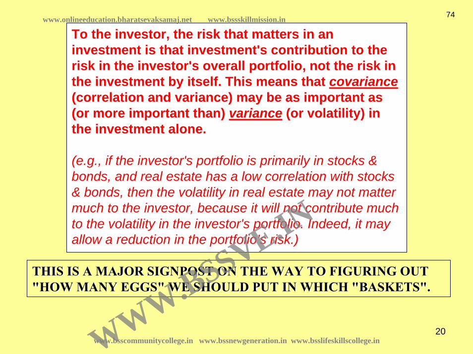
20
To the investor, the risk that matters in an investment is that investment's contribution to the risk in the investor's overall portfolio, not the risk in the investment by itself. This means that covariance(correlation and variance) may be as important as (or more important than) variance (or volatility) in the investment alone.
(e.g., if the investor's portfolio is primarily in stocks & bonds, and real estate has a low correlation with stocks & bonds, then the volatility in real estate may not matter much to the investor, because it will not contribute much to the volatility in the investor's portfolio. Indeed, it may allow a reduction in the portfolio’s risk.)
THIS IS A MAJOR SIGNPOST ON THE WAY TO FIGURING OUT THIS IS A MAJOR SIGNPOST ON THE WAY TO FIGURING OUT "HOW MANY EGGS" WE SHOULD PUT IN WHICH "BASKETS"."HOW MANY EGGS" WE SHOULD PUT IN WHICH "BASKETS".
www.bsscommunitycollege.in www.bssnewgeneration.in www.bsslifeskillscollege.in
74www.onlineeducation.bharatsevaksamaj.net www.bssskillmission.in
WWW.BSSVE.IN

21
21.2.4 STEP 1: FINDING THE EFFICIENT FRONTIER
SUPPOSE WE HAVE THE FOLLOWING RISK & RETURN EXPECTATIONS…
INVESTING IN ANY ONE OF THE THREE ASSET CLASSES WITHOUT DIVERSIFICATION ALLOWS THE INVESTOR TO ACHIEVE ONLY ONE OF THREE POSSIBLE RISK/RETURN POINTS…
Stocks Bonds REMean 10.00% 6.00% 7.00%STD 15.00% 8.00% 10.00%CorrStocks 100.00% 30.00% 25.00%Bonds 100.00% 15.00%RE 100.00%
www.bsscommunitycollege.in www.bssnewgeneration.in www.bsslifeskillscollege.in
75www.onlineeducation.bharatsevaksamaj.net www.bssskillmission.in
WWW.BSSVE.IN

22
INVESTING IN ANY ONE OF THE THREE ASSET CLASSES WITHOUT INVESTING IN ANY ONE OF THE THREE ASSET CLASSES WITHOUT DIVERSIFICATION ALLOWS THE INVESTOR TO ACHIEVE ONLY ONE OF DIVERSIFICATION ALLOWS THE INVESTOR TO ACHIEVE ONLY ONE OF THE THREE POSSIBLE RISK/RETURN POINTS DEPICTED IN THE GRAPH THE THREE POSSIBLE RISK/RETURN POINTS DEPICTED IN THE GRAPH BELOWBELOW……
IN A RISK/RETURN CHART LIKE THIS, ONE WANTS TO BE ABLE TO GET ASMANY RISK/RETURN COMBINATIONS AS POSSIBLE, AS FAR TO THE “NORTH” AND “WEST” AS POSSIBLE.
3 Assets: Stocks, Bonds, RE, No Diversification
4%
6%
8%
10%
12%
6% 8% 10% 12% 14% 16%
Risk (Std.Dev)
E(r)
Stocks Bonds Real Ests
Bonds
Real Est
Stocks
www.bsscommunitycollege.in www.bssnewgeneration.in www.bsslifeskillscollege.in
76www.onlineeducation.bharatsevaksamaj.net www.bssskillmission.in
WWW.BSSVE.IN

23
ALLOWING PAIRWISE COMBINATIONS (AS WITH OUR PREVIOUS STOCKS ALLOWING PAIRWISE COMBINATIONS (AS WITH OUR PREVIOUS STOCKS & REAL ESTATE EXAMPLE), INCREASES THE RISK/RETURN & REAL ESTATE EXAMPLE), INCREASES THE RISK/RETURN POSSIBILITIES TO THESEPOSSIBILITIES TO THESE……
3 Assets: Stocks, Bonds, RE, with pairwise combinations
4%
6%
8%
10%
12%
6% 8% 10% 12% 14% 16%
Risk (Std.Dev)
E(r)
RE&Stocks Stks&Bonds RE&Bonds
Bonds
Real Est
Stocks
www.bsscommunitycollege.in www.bssnewgeneration.in www.bsslifeskillscollege.in
77www.onlineeducation.bharatsevaksamaj.net www.bssskillmission.in
WWW.BSSVE.IN

24
FINALLY, IF WE ALLOW UNLIMITED DIVERSIFICATION AMONG ALL THREE FINALLY, IF WE ALLOW UNLIMITED DIVERSIFICATION AMONG ALL THREE ASSET CLASSES, WE ENABLE AN INFINITE NUMBER OF COMBINATIONS, ASSET CLASSES, WE ENABLE AN INFINITE NUMBER OF COMBINATIONS, THE THE ““BESTBEST”” (I.E., MOST (I.E., MOST ““NORTHNORTH”” AND AND ““WESTWEST””) OF WHICH ARE SHOWN ) OF WHICH ARE SHOWN BY THE OUTSIDE (ENVELOPING) CURVE.BY THE OUTSIDE (ENVELOPING) CURVE.
THIS IS THE “EFFICIENT FRONTIER” IN THIS CASE (OF THREE ASSET CLASSES).
3 Assets with Diversification: The Efficient Frontier
4%
6%
8%
10%
12%
6% 8% 10% 12% 14% 16%
Risk (Std.Dev)
E(r)
Effic.Frontier RE&Stocks Stks&Bonds RE&Bonds
www.bsscommunitycollege.in www.bssnewgeneration.in www.bsslifeskillscollege.in
78www.onlineeducation.bharatsevaksamaj.net www.bssskillmission.in
WWW.BSSVE.IN

25
IN PORTFOLIO THEORY THE IN PORTFOLIO THEORY THE ““EFFICIENT FRONTIEREFFICIENT FRONTIER””CONSISTS OF ALL ASSET COMBINATIONS CONSISTS OF ALL ASSET COMBINATIONS (PORTFOLIOS) WHICH MAXIMIZE RETURN AND (PORTFOLIOS) WHICH MAXIMIZE RETURN AND MINIMIZE RISK. MINIMIZE RISK. THE EFFICIENT FRONTIER IS AS FAR THE EFFICIENT FRONTIER IS AS FAR ““NORTHNORTH”” AND AND ““WESTWEST”” AS YOU CAN POSSIBLY GET IN THE AS YOU CAN POSSIBLY GET IN THE RISK/RETURN GRAPH.RISK/RETURN GRAPH.
(Terminology note: This is a different definition of "efficiency(Terminology note: This is a different definition of "efficiency" " than the concept of informational efficiency applied to asset than the concept of informational efficiency applied to asset markets and asset prices.)markets and asset prices.)
A PORTFOLIO IS SAID TO BE A PORTFOLIO IS SAID TO BE ““EFFICIENTEFFICIENT”” (i.e., (i.e., represents one point on the efficient frontier) IF IT HAS THE represents one point on the efficient frontier) IF IT HAS THE MINIMUM POSSIBLE VOLATILITY FOR A GIVEN MINIMUM POSSIBLE VOLATILITY FOR A GIVEN EXPECTED RETURN, AND/OR THE MAXIMUM EXPECTED RETURN, AND/OR THE MAXIMUM EXPECTED RETURN FOR A GIVEN LEVEL OF EXPECTED RETURN FOR A GIVEN LEVEL OF VOLATILITY.VOLATILITY.
www.bsscommunitycollege.in www.bssnewgeneration.in www.bsslifeskillscollege.in
79www.onlineeducation.bharatsevaksamaj.net www.bssskillmission.in
WWW.BSSVE.IN
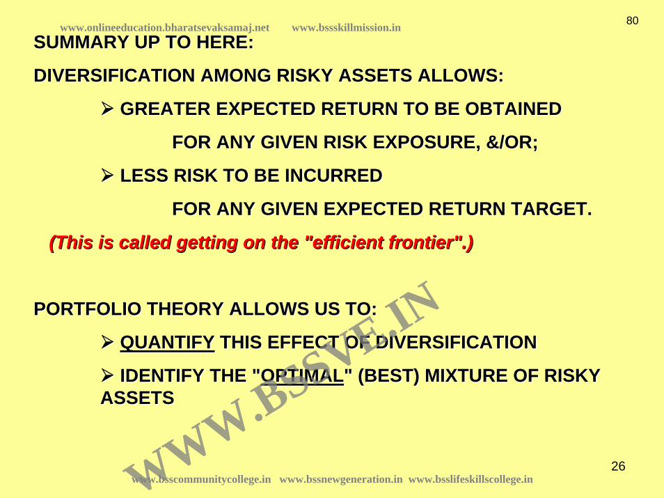
26
SUMMARY UP TO HERE:SUMMARY UP TO HERE:
DIVERSIFICATION AMONG RISKY ASSETS ALLOWS:DIVERSIFICATION AMONG RISKY ASSETS ALLOWS:
GREATER EXPECTED RETURN TO BE OBTAINEDGREATER EXPECTED RETURN TO BE OBTAINED
FOR ANY GIVEN RISK EXPOSURE, &/OR;FOR ANY GIVEN RISK EXPOSURE, &/OR;
LESS RISK TO BE INCURREDLESS RISK TO BE INCURRED
FOR ANY GIVEN EXPECTED RETURN TARGET.FOR ANY GIVEN EXPECTED RETURN TARGET.
(This is called getting on the "efficient frontier".)(This is called getting on the "efficient frontier".)
PORTFOLIO THEORY ALLOWS US TO:PORTFOLIO THEORY ALLOWS US TO:
QUANTIFYQUANTIFY THIS EFFECT OF DIVERSIFICATIONTHIS EFFECT OF DIVERSIFICATION
IDENTIFY THE "IDENTIFY THE "OPTIMALOPTIMAL" (BEST) MIXTURE OF RISKY " (BEST) MIXTURE OF RISKY ASSETSASSETS
www.bsscommunitycollege.in www.bssnewgeneration.in www.bsslifeskillscollege.in
80www.onlineeducation.bharatsevaksamaj.net www.bssskillmission.in
WWW.BSSVE.IN

27
MATHEMATICALLY, THIS IS A "CONSTRAINED MATHEMATICALLY, THIS IS A "CONSTRAINED OPTIMIZATION" PROBLEMOPTIMIZATION" PROBLEM
==> Algebraic solution using calculus==> Algebraic solution using calculus
==> Numerical solution using computer and ==> Numerical solution using computer and "quadratic programming". Spreadsheets such as Excel "quadratic programming". Spreadsheets such as Excel include "Solvers" that can find optimal portfolios this include "Solvers" that can find optimal portfolios this way.way.
www.bsscommunitycollege.in www.bssnewgeneration.in www.bsslifeskillscollege.in
81www.onlineeducation.bharatsevaksamaj.net www.bssskillmission.in
WWW.BSSVE.IN

28
21.2.5. STEP 2: PICK A RETURN TARGET FOR YOUR OVERALL WEALTH THAT REFLECTS YOUR RISK PREFERENCES...
E.G., ARE YOU HERE (7%)?...E.G., ARE YOU HERE (7%)?...
Optimal portfolio (P) for a conservative investor: Target=7%
4%
6%
8%
10%
12%
6% 8% 10% 12% 14% 16%
Risk (Std.Dev)
E(r)
P = 16%St, 48%Bd, 36%RE for 7% Target
maxrisk/returnindifferencecurve
Eff icientFrontier
www.bsscommunitycollege.in www.bssnewgeneration.in www.bsslifeskillscollege.in
82www.onlineeducation.bharatsevaksamaj.net www.bssskillmission.in
WWW.BSSVE.IN
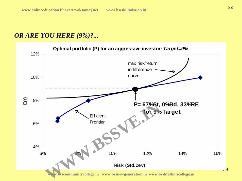
29
OR ARE YOU HERE (9%)?...OR ARE YOU HERE (9%)?...
Optimal portfolio (P) for an aggressive investor: Target=9%
4%
6%
8%
10%
12%
6% 8% 10% 12% 14% 16%
Risk (Std.Dev)
E(r)
P= 67%St, 0%Bd, 33%RE for 9% Target
max risk/return indifference curve
Eff icientFrontier
www.bsscommunitycollege.in www.bssnewgeneration.in www.bsslifeskillscollege.in
83www.onlineeducation.bharatsevaksamaj.net www.bssskillmission.in
WWW.BSSVE.IN

30
21.2.6 Major Implications of Portfolio Theory for Real Estate Investment
ASSET COMPOSITION OF THE EFFICIENT FRONTIER(based on Exhibit 21-1a expectations)
0%
25%
50%
75%
100%
6.0% 7.0% 8.0% 9.0% 10.0%
INVESTOR RETURN TARGET
RE Share
Bond Share
StockShare
Core real estate assets typically make up a large share of efficCore real estate assets typically make up a large share of efficient ient (non(non--dominated) portfolios for conservative to moderate return dominated) portfolios for conservative to moderate return
targets.targets.www.bsscommunitycollege.in www.bssnewgeneration.in www.bsslifeskillscollege.in
84www.onlineeducation.bharatsevaksamaj.net www.bssskillmission.in
WWW.BSSVE.IN

31
GENERAL QUALITATIVE RESULTS OF PORTFOLIO THEORY
1) THE OPTIMAL REAL ESTATE SHARE DEPENDS ON HOW CONSERVATIVE OR AGGRESSIVE IS THE INVESTOR;
2) FOR MOST OF THE RANGE OF RETURN TARGETS, REAL ESTATE IS A SIGNIFICANT SHARE. (COMPARE THESE SHARES TO THE AVERAGE U.S. PENSION FUND REAL ESTATE ALLOCATION WHICH IS LESS THAN 5%. THIS IS WHY PORTFOLIO THEORY HAS BEEN USED TO TRY TO GET INCREASED PF ALLOCATION TO REAL ESTATE.)
3) THE ROBUSTNESS OF REAL ESTATE'S INVESTMENT APPEAL IS DUE TO ITS LOW CORRELATION WITH BOTH STOCKS & BONDS, THAT IS, WITH ALL OF THE REST OF THE PORTFOLIO. (NOTE IN PARTICULAR THAT OUR INPUT ASSUMPTIONS IN THE ABOVE EXAMPLE NUMBERS DID NOT INCLUDE A PARTICULARLY HIGH RETURN OR PARTICULARLY LOW VOLATILITY FOR THE REAL ESTATE ASSET CLASS. THUS, THE LARGE REAL ESTATE SHARE IN THE OPTIMAL PORTFOLIO MUST NOT BE DUE TO SUCH ASSUMPTIONS.)
www.bsscommunitycollege.in www.bssnewgeneration.in www.bsslifeskillscollege.in
85www.onlineeducation.bharatsevaksamaj.net www.bssskillmission.in
WWW.BSSVE.IN

32
Exhibit 21-9a: Possible Risk & Return Expectations for 5 Asset Classes
Large Stocks Small Stocks
Bonds REITs Private Real Estate
Expected Return (E[r]) 10.00% 12.00% 6.00% 10.00% 7.00%
Volatility 15.00% 20.00% 8.00% 15.00% 10.00% Correlation with: Large Stocks 100.00% 60.00% 30.00% 45.00% 25.00% Small Stocks 100.00% 0.00% 70.00% 25.00% Bonds 100.00% 20.00% 15.00% REITs 100.00% 40.00% Private Real Estate 100.00%
21.2.7 SUPPOSE WE EXPAND THE PORTFOLIO CHOICE SET BY ADDING ADDITIONAL SUB-CLASSES OF ASSETS…
For example, suppose we add the following expectations for an additional sub-class of stocks (small stocks) and an additional sub-class of real estate (REITs)…
www.bsscommunitycollege.in www.bssnewgeneration.in www.bsslifeskillscollege.in
86www.onlineeducation.bharatsevaksamaj.net www.bssskillmission.in
WWW.BSSVE.IN

33
ASSET COMPOSITION OF THE EFFICIENT FRONTIER(based on Exhibit 21-9a expectations)
0%
25%
50%
75%
100%
6.0% 7.5% 9.0% 10.5% 12.0%
INVESTOR RETURN TARGET
Private RealEstate
REITs
Bonds
SmallStocks
LargeStocks
www.bsscommunitycollege.in www.bssnewgeneration.in www.bsslifeskillscollege.in
87www.onlineeducation.bharatsevaksamaj.net www.bssskillmission.in
WWW.BSSVE.IN

34
VII. INTRODUCING A "RISKLESS ASSET"... IN A COMBINATION OF A RISKLESS AND A RISKY ASSET, BOTH RISK AND RETURN ARE WEIGHTED AVERAGES OF RISK AND RETURN OF THE TWO ASSETS: Recall: sP = √[ ω²(si)² + (1-ω)²(sj)² + 2ω(1-ω)sisjCij ] If sj=0, this reduces to: sP = √[ ω²(si)² = ωsi SO THE RISK/RETURN COMBINATIONS OF A MIXTURE OF INVESTMENT IN A RISKLESS ASSET AND A RISKY ASSET LIE ON A STRAIGHT LINE, PASSING THROUGH THE TWO POINTS REPRESENTING THE RISK/RETURN COMBINATIONS OF THE RISKLESS ASSET AND THE RISKY ASSET.
Section 21.3Section 21.3
www.bsscommunitycollege.in www.bssnewgeneration.in www.bsslifeskillscollege.in
88www.onlineeducation.bharatsevaksamaj.net www.bssskillmission.in
WWW.BSSVE.IN

35
VolatilityVolatilityssii ssjj
EE[[rrjj]]
EE[[rrii]]
If either i or j is riskless . . .
www.bsscommunitycollege.in www.bssnewgeneration.in www.bsslifeskillscollege.in
89www.onlineeducation.bharatsevaksamaj.net www.bssskillmission.in
WWW.BSSVE.IN

36
IN PORTFOLIO ANALYSIS, THE "RISKLESS ASSET" REPRESENTS BORROWING OR LENDING BY THE INVESTOR… BORROWING IS LIKE "SELLING SHORT" OR HOLDING A NEGATIVE WEIGHT IN THE RISKLESS ASSET. BORROWING IS "RISKLESS" BECAUSE YOU MUST PAY THE MONEY BACK “NO MATTER WHAT”. LENDING IS LIKE BUYING A BOND OR HOLDING A POSITIVE WEIGHT IN THE RISKLESS ASSET. LENDING IS "RISKLESS" BECAUSE YOU CAN INVEST IN GOVT BONDS AND HOLD TO MATURITY.
www.bsscommunitycollege.in www.bssnewgeneration.in www.bsslifeskillscollege.in
90www.onlineeducation.bharatsevaksamaj.net www.bssskillmission.in
WWW.BSSVE.IN

37
SUPPOSE YOU COMBINE RISKLESS BORROWING OR LENDING WITH YOUR INVESTMENT IN THE RISKY PORTFOLIO OF STOCKS & REAL ESTATE. YOUR OVERALL EXPECTED RETURN WILL BE: rW = vrP + (1-v)rf AND YOUR OVERALL RISK WILL BE: sW = vsP + (1-v)0 = vsP Where: v = Weight in risky portfolio rW, sW = Return, Std.Dev., in overall wealth rP, sP = Return, Std.Dev., in risky portfolio rf = Riskfree Interest Rate v NEED NOT BE CONSTRAINED TO BE LESS THAN UNITY. v CAN BE GREATER THAN 1 ("leverage" , "borrowing"), OR v CAN BE LESS THAN 1 BUT POSITIVE ("lending", investing in bonds, in addition to investing in the risky portfolio). THUS, USING BORROWING OR LENDING, IT IS POSSIBLE TO OBTAIN ANY RETURN TARGET OR ANY RISK TARGET. THE RISK/RETURN COMBINATIONS WILL LIE ON THE STRAIGHT LINE PASSING THROUGH POINTS rf AND rP.
www.bsscommunitycollege.in www.bssnewgeneration.in www.bsslifeskillscollege.in
91www.onlineeducation.bharatsevaksamaj.net www.bssskillmission.in
WWW.BSSVE.IN

38
NUMERICAL EXAMPLE SUPPOSE: RISKFREE INTEREST RATE = 5% STOCK EXPECTED RETURN = 15% STOCK STD.DEV. = 15% ________________________________________________________ IF RETURN TARGET = 20%, BORROW $0.5 INVEST $1.5 IN STOCKS (v = 1.5). EXPECTED RETURN WOULD BE: (1.5)15% + (-0.5)5% = 20% RISK WOULD BE (1.5)15% + (-0.5)0% = 22.5% ________________________________________________________ IF RETURN TARGET = 10%, LEND (INVEST IN BONDS) $0.5 INVEST $0.5 IN STOCKS (v = 0.5). EXPECTED RETURN WOULD BE: (0.5)15% + (0.5)5% = 10% RISK WOULD BE (0.5)15% + (0.5)0% = 7.5% ___________________________________________________________www.bsscommunitycollege.in www.bssnewgeneration.in www.bsslifeskillscollege.in
92www.onlineeducation.bharatsevaksamaj.net www.bssskillmission.in
WWW.BSSVE.IN

39
NOTICE THESE POSSIBILITIES LIE ON A STRAIGHT LINE IN RISK/RETURN SPACE . . .
0% 7.5% 15% 22.5%0%
5%
10%
15%
20%
25%
30%
35%RISK & RETURN COMBINATIONS USING STOCKS & RISKLESS BORROWING OR LENDI
RISK (STD.DEV.)
EXPCTEDRETURN
V = WEIGHT IN STOCKSV=0
V=50%
V=150%
V=100%
BORROW
LEND
www.bsscommunitycollege.in www.bssnewgeneration.in www.bsslifeskillscollege.in
93www.onlineeducation.bharatsevaksamaj.net www.bssskillmission.in
WWW.BSSVE.IN

40
BUT NO MATTER WHAT YOUR RETURN TARGET, YOU CAN DO BETTER BY PUTTING YOUR RISKY MONEY IN A DIVERSIFIED PORTFOLIO OF REAL ESTATE & STOCKS . . . SUPPOSE: REAL ESTATE EXPECTED RETURN = 10% REAL ESTATE STD.DEV. = 10% CORRELATION BETWEEN STOCKS & REAL ESTATE = 25% THEN 50% R.E. / STOCKS MIXTURE WOULD PROVIDE: EXPECTED RETURN = 12.5%; STD.DEV. = 10.0% ________________________________________________________ IF RETURN TARGET = 20%, BORROW $1.0 INVEST $2.0 IN RISKY MIXED-ASSET PORTFOLIO (v = 2). EXPECTED RETURN WOULD BE: (2.0)12.5% + (-1.0)5% = 20% RISK WOULD BE: (2.0)10.0% + (-1.0)0% = 20% < 22.5% _______________________________________________________ IF RETURN TARGET = 10%, LEND (INVEST IN BONDS) $0.33 INVEST $0.67 IN RISKY MIXED-ASSET PORTFOLIO (v = 0.67). EXPECTED RETURN WOULD BE: (0.67)12.5% + (0.33)5% = 10% RISK WOULD BE: (0.67)10.0% + (0.33)0% = 6.7% < 7.5%
www.bsscommunitycollege.in www.bssnewgeneration.in www.bsslifeskillscollege.in
94www.onlineeducation.bharatsevaksamaj.net www.bssskillmission.in
WWW.BSSVE.IN

41
THE GRAPH BELOW SHOWS THE EFFECT DIVERSIFICATION IN THE RISKY PORTFOLIO HAS ON THE RISK/RETURN POSSIBILITY FRONTIER.
0%
5%
10%
15%
20%
25%
0% 5% 10% 15% 20% 25%Risk in overall wealth portfolio
Expt
d R
etur
n
Effect of diversif ication: Stocks, R.E., & Riskless Asset
THE FRONTIER IS STILL A STRAIGHT LINE ANCHORED ON THE RISKFREE RATE, BUT THE LINE NOW HAS A GREATER “SLOPE”, PROVIDING MORE RETURN FOR THE SAME AMOUNT OF RISK, ALLOWING LESS RISK FOR THE SAME EXPECTED RETURN.
www.bsscommunitycollege.in www.bssnewgeneration.in www.bsslifeskillscollege.in
95www.onlineeducation.bharatsevaksamaj.net www.bssskillmission.in
WWW.BSSVE.IN

42
THE "OPTIMAL" RISKY ASSET PORTFOLIO WITH A RISKLESS ASSET
(aka "TWO-FUND THEOREM")
CURVED LINE IS FRONTIER OBTAINABLE INVESTING ONLY IN RISKY ASSETS STRAIGHT LINE PASSING THRU rf AND PARABOLA IS OBTAINABLE BY MIXING RISKLESS ASSET (LONG OR SHORT) WITH RISKY ASSETS. YOU WANT “HIGHEST” STRAIGHT LINE POSSIBLE (NO MATTER WHO YOU ARE!). OPTIMAL STRAIGHT LINE IS THUS THE ONE PASSING THRU POINT "P". IT IS THE STRAIGHT LINE ANCHORED IN rf WITH THE MAXIMUM POSSIBLE SLOPE. THUS, THE STRAIGHT LINE PASSING THROUGH “P” IS THE EFFICIENT FRONTIER. THE FRONTIER TOUCHES (AND INCLUDES) THE CURVED LINE AT ONLY ONE POINT: THE POINT "P".
rf
i
j
P
rj
rP
ri
Risk(Std.Dev.of Portf)
E[Return]
www.bsscommunitycollege.in www.bssnewgeneration.in www.bsslifeskillscollege.in
96www.onlineeducation.bharatsevaksamaj.net www.bssskillmission.in
WWW.BSSVE.IN

43
THUS, THE "2-FUND THEOREM" TELLS US THAT THERE IS A SINGLE PARTICULAR COMBINATION OF RISKY ASSETS (THE PORTFOLIO “P”) WHICH IS "OPTIMAL" NO MATTER WHAT THE INVESTOR'S RISK PREFERENCES OR TARGET RETURN.
THUS, ALL EFFIC. PORTFS ARE COMBINATIONS OF JUST 2 FUNDS: RISKLESS FUND (long or short position) + RISKY FUND "P" (long position). HENCE THE NAME: "2-FUND THEOREM".
rf
i
j
P
rj
rP
ri
Risk(Std.Dev.of Portf)
E[Return]
www.bsscommunitycollege.in www.bssnewgeneration.in www.bsslifeskillscollege.in
97www.onlineeducation.bharatsevaksamaj.net www.bssskillmission.in
WWW.BSSVE.IN

44
HOW DO WE KNOW WHICH COMBINATION OF RISKY ASSETS IS THE OPTIMAL ALL-RISKY PORTFOLIO “P”? IT IS THE ONE THAT MAXIMIZES THE SLOPE OF THE STRAIGHT LINE FROM THE RISKFREE RETURN THROUGH “P”. THE SLOPE OF THIS LINE IS GIVEN BY THE RATIO: Portfolio Sharpe Ratio = (rp - rf) / sP MAXIMIZING THE SHARPE RATIO FINDS THE OPTIMAL RISKY ASSET COMBINATION. THE SHARPE RATIO IS ALSO A GOOD INTUITIVE MEASURE OF “RISK-ADJUSTED RETURN” FOR THE INVESTOR’S WEALTH, AS IT GIVES THE RISK PREMIUM PER UNIT OF RISK (MEASURED BY ST.DEV). THUS, IF WE ASSUME THE EXISTENCE OF A RISKLESS ASSET, WE CAN USE THE 2-FUND THEOREM TO FIND THE OPTIMAL RISKY ASSET MIXTURE AS THAT PORTFOLIO WHICH HAS THE HIGHEST "SHARPE RATIO".
21.3.221.3.2
www.bsscommunitycollege.in www.bssnewgeneration.in www.bsslifeskillscollege.in
98www.onlineeducation.bharatsevaksamaj.net www.bssskillmission.in
WWW.BSSVE.IN

45
BACK TO PREVIOUS 2-ASSET NUMERICAL EXAMPLE... USING OUR PREVIOUS EXAMPLE NUMBERS, THE OPTIMAL COMBINATION OF REAL ESTATE & STOCKS CAN BE FOUND BY EXAMINING THE SHARPE RATIO FOR EACH COMBINATION . . . ω = RE share
rP rp-rf sP SharpeRatio
0 15.0% 10.0% 15.0% 66.7%0.1 14.5% 9.5% 13.8% 68.9%0.2 14.0% 9.0% 12.6% 71.2%0.3 13.5% 8.5% 11.6% 73.2%0.4 13.0% 8.0% 10.7% 74.6%0.5 12.5% 7.5% 10.0% 75.0%0.6 12.0% 7.0% 9.5% 73.8%0.7 11.5% 6.5% 9.2% 70.5%0.8 11.0% 6.0% 9.2% 65.1%0.9 10.5% 5.5% 9.5% 58.0%1.0 10.0% 5.0% 10.0% 50.0% OF THE 11 MIXTURES CONSIDERED ABOVE, THE 50% REAL ESTATE WOULD BE BEST BECAUSE IT HAS THE HIGHEST SHARPE MEASURE. BUT SUPPOSE YOU ARE NOT SATISFIED WITH THE 12.5% Er THAT WILL GIVE YOU FOR YOUR OVERALL WEALTH? … OR YOU DON’T WANT TO SUBJECT YOUR OVERALL WEALTH TO 10% VOLATILITY?...
www.bsscommunitycollege.in www.bssnewgeneration.in www.bsslifeskillscollege.in
99www.onlineeducation.bharatsevaksamaj.net www.bssskillmission.in
WWW.BSSVE.IN

46
THEN YOU CAN INVEST PROPORTIONATELY 50% IN REAL ESTATE AND 50% IN STOCKS, … AND THEN ACHIEVE A GREATER RETURN THAN 12.5% BY BORROWING (LEVERAGE, v > 1), OR YOU CAN INCUR LESS THAN 10.0% RISK BY LENDING (INVESTING IN GOVT BONDS, v<1)… (BUT YOU CAN’T DO BOTH. THE “FREE LUNCH” OF PORTFOLIO THEORY ONLY GETS YOU SO FAR, THAT IS, TO THE EFFICIENT FRONTIER, BUT ON THAT FRONTIER THERE WILL BE A RISK/RETURN TRADEOFF. THAT TRADEOFF WILL BE DETERMINED BY THE MARKET…)
www.bsscommunitycollege.in www.bssnewgeneration.in www.bsslifeskillscollege.in
100www.onlineeducation.bharatsevaksamaj.net www.bssskillmission.in
WWW.BSSVE.IN

47
Exhibit 21-11: Comparison of Optimal 7%-Return-Target Portfolio Allocations, Variance-Minimization vs Sharpe Ratio-Maximization...
Return & Risk Expectations*: Portfolio Allocations:
Return VolatilitySharpe
Ratio Var-Min Sharpe-MaxCash (T-bills) 3.00% NA** NA NA 10%Bonds 6.00% 8.00% 0.38 48% 33%Real Estate 7.00% 10.00% 0.40 36% 32%Stocks 10.00% 15.00% 0.47 16% 25%Var-Min Portfolio 7.00% 6.89% 0.58 100% NAShape-Max Portf. 7.00% NA** 0.59 NA 100%*Also includes correlations: Stock-Bond +30%, Stock-Real Estate +25%, Bond-Real Estate +15%. **From the Sharpe-maximization perspective, T-bills are viewed as having zero volatility, but as this is not exactly true in reality, it would be misleading to calculate and show a Sharpe-maximizing portfolio volatility juxtaposed with that of the variance-minimized portfolio.
Example of Difference Between Markowitz and Sharpe Optimal Portfolios
www.bsscommunitycollege.in www.bssnewgeneration.in www.bsslifeskillscollege.in
101www.onlineeducation.bharatsevaksamaj.net www.bssskillmission.in
WWW.BSSVE.IN

48
2-FUND THEOREM SUMMARY: 1) THE 2-FUND THEOREM ALLOWS AN ALTERNATIVE,
INTUITIVELY APPEALING DEFINITION OF THE OPTIMAL RISKY PORTFOLIO: THE ONE WITH THE MAXIMUM SHARPE RATIO.
2) THIS CAN HELP AVOID "SILLY" OPTIMAL PORTFOLIOS
THAT PUT TOO LITTLE WEIGHT IN HIGH-RETURN ASSETS JUST BECAUSE THE INVESTOR HAS A CONSERVATIVE TARGET RETURN. (OR TOO LITTLE WEIGHT IN LOW-RETURN ASSETS JUST BECAUSE THE INVESTOR HAS AN AGGRESSIVE TARGET.)
3) IT ALSO PROVIDES A GOOD FRAMEWORK FOR
ACCOMMODATING THE POSSIBLE USE OF LEVERAGE, OR OF RISKLESS INVESTING (BY HOLDING BONDS TO MATURITY), BY THE INVESTOR.
www.bsscommunitycollege.in www.bssnewgeneration.in www.bsslifeskillscollege.in
102www.onlineeducation.bharatsevaksamaj.net www.bssskillmission.in
WWW.BSSVE.IN

49
Chapter 21 Summary: MPT & Real Estate . . .Chapter 21 Summary: MPT & Real Estate . . .•• The classical theory suggests a fairly robust, substantial roleThe classical theory suggests a fairly robust, substantial role for the real estate for the real estate asset class in the optimal portfolio (typically 25%asset class in the optimal portfolio (typically 25%--40% without any additional 40% without any additional assumptions), either w or w/out assumptions), either w or w/out risklessriskless asset.asset.•• This role tends to be greater for more conservative portfolios,This role tends to be greater for more conservative portfolios, less for very less for very aggressive portfolios.aggressive portfolios.•• Role is based primarily on Role is based primarily on diversification benefitsdiversification benefits of real estate, somewhat of real estate, somewhat sensitive to R.E. correlation w stocks & bonds.sensitive to R.E. correlation w stocks & bonds.•• Optimal real estate share roughly matches actual real estate prOptimal real estate share roughly matches actual real estate proportion of all oportion of all investableinvestable assets in the economy.assets in the economy.•• Optimal real estate share in theory is substantially greater thOptimal real estate share in theory is substantially greater than actual pension an actual pension fund allocations to real estate.fund allocations to real estate.•• Optimal R.E. share can be reduced by adding assumptions and extOptimal R.E. share can be reduced by adding assumptions and extensions to the ensions to the classical model:classical model:
• Extra transaction costs, illiquidity penalties;• Long-term horizon risk & returns;• Net Asset-Liability portfolio framework;• Investor constrained to over-invest in owner-occupied house as investment.
•• But even with such extensions, optimal R.E. share often substanBut even with such extensions, optimal R.E. share often substantially exceeds tially exceeds existing P.F. allocations to R.E. (approx. 3% on avg.*)existing P.F. allocations to R.E. (approx. 3% on avg.*)
www.bsscommunitycollege.in www.bssnewgeneration.in www.bsslifeskillscollege.in
103www.onlineeducation.bharatsevaksamaj.net www.bssskillmission.in
WWW.BSSVE.IN

50
Chapter 22Chapter 22Equilibrium Asset PricingEquilibrium Asset Pricing
www.bsscommunitycollege.in www.bssnewgeneration.in www.bsslifeskillscollege.in
104www.onlineeducation.bharatsevaksamaj.net www.bssskillmission.in
WWW.BSSVE.IN
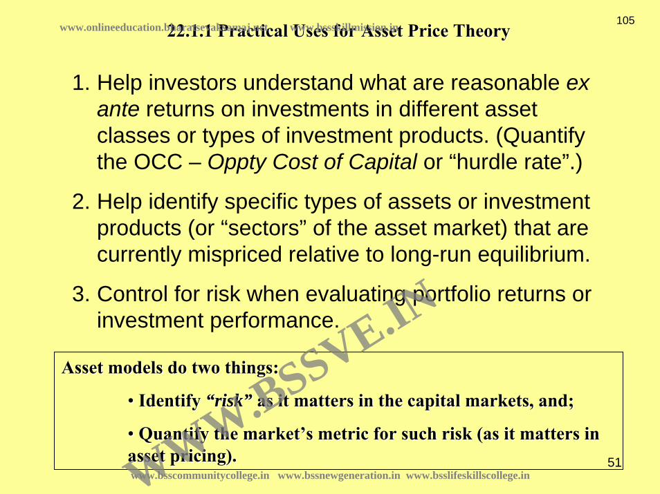
51
1. Help investors understand what are reasonable ex ante returns on investments in different asset classes or types of investment products. (Quantify the OCC – Oppty Cost of Capital or “hurdle rate”.)
2. Help identify specific types of assets or investment products (or “sectors” of the asset market) that are currently mispriced relative to long-run equilibrium.
3. Control for risk when evaluating portfolio returns or investment performance.
22.1.1 Practical Uses for Asset Price Theory 22.1.1 Practical Uses for Asset Price Theory
Asset models do two things:Asset models do two things:
•• Identify Identify ““riskrisk”” as it matters in the capital markets, and;as it matters in the capital markets, and;
•• Quantify the marketQuantify the market’’s metric for such risk (as it matters in s metric for such risk (as it matters in asset pricing).asset pricing).www.bsscommunitycollege.in www.bssnewgeneration.in www.bsslifeskillscollege.in
105www.onlineeducation.bharatsevaksamaj.net www.bssskillmission.in
WWW.BSSVE.IN

52
Simulated Historical Present Values
Using VAR-Forecasted Cash Flows (CF) & Returns (R) in Present Value Model
0.8
0.9
1.0
1.1
1.2
1.3
1.4
1.5
1.6
1.7
1.8
1975 1976 1977 1978 1979 1980 1981 1982 1983 1984 1985 1986 1987 1988 1989 1990 1991 1992
Source: Geltner & Mei (1995)
Both CF & R Variable CF Constant, R Variable CF Variable, R Constant
22.1.2 A Threshold Point: What Underlies Asset Risk?
Most of the volatility in asset prices does not derive Most of the volatility in asset prices does not derive from rational changes in future cash flow expectationsfrom rational changes in future cash flow expectations
www.bsscommunitycollege.in www.bssnewgeneration.in www.bsslifeskillscollege.in
106www.onlineeducation.bharatsevaksamaj.net www.bssskillmission.in
WWW.BSSVE.IN

53
VIII. FROM PORTFOLIO THEORY TO EQUILIBRIUM ASSET PRICE MODELLING...
HOW ASSET MARKET PRICES ARE DETERMINED. i.e., WHAT SHOULD BE “E[r]” FOR ANY GIVEN ASSET?… RECALL RELATION BETW “PV” AND “E[r]”.
e.g., for perpetutity: PV = CF / E[r]
(A model of price is a model of expected return, and vice versa, a model of expected return is a model of price.)
THUS, ASSET PRICING MODEL CAN IDENTIFY “MISPRICED” ASSETS (ASSETS WHOSE “E[r]” IS ABOVE OR BELOW WHAT IT SHOULD BE, THAT IS, ASSETS WHOSE CURRENT “MVs” ARE “WRONG”, AND WILL PRESUMABLY TEND TO “GET CORRECTED” IN THE MKT OVER TIME). IF PRICE (HENCE E[r]) OF ANY ASSET DIFFERS FROM WHAT THE MODEL PREDICTS, THE IMPLICATION IS THAT THE PRICE OF THAT ASSET WILL TEND TO REVERT TOWARD WHAT THE MODEL PREDICTS, THEREBY ALLOWING PREDICTION OF SUPER-NORMAL OR SUB-NORMAL RETURNS FOR SPECIFIC ASSETS, WITH OBVIOUS INVESTMENT POLICY IMPLICATIONS.
22.1.322.1.3
www.bsscommunitycollege.in www.bssnewgeneration.in www.bsslifeskillscollege.in
107www.onlineeducation.bharatsevaksamaj.net www.bssskillmission.in
WWW.BSSVE.IN

54
Quick & simple example… Suppose model predicts E[r] for $10 perpetuity asset should be 10%. This means equilibrium price of this asset should be $100. But you find an asset like this whose price is $83. This means it is providing an E[r] of 12% ( = 10 / 83 ). Thus, if model is correct, you should buy this asset for $83. Because at that price it is providing a “supernormal” return, and because we would expect that as prices move toward equilibrium the value of this asset will move toward $100 from its current $83 price. (i.e., You will get your supernormal return either by continuing to receive a 12% yield when the risk only warrants a 10% yield, or else by the asset price moving up in equilibrium providing a capital gain “pop”.)
www.bsscommunitycollege.in www.bssnewgeneration.in www.bsslifeskillscollege.in
108www.onlineeducation.bharatsevaksamaj.net www.bssskillmission.in
WWW.BSSVE.IN

55
THE "SHARPE-LINTNER CAPM" (in 4 easy steps!)… (Nobel prize-winning stuff here – Show some respect!) 1ST) 2-FUND THEOREM SUGGESTS THERE IS A SINGLE COMBINATION OF RISKY ASSETS THAT YOU SHOULD HOLD, NO MATTER WHAT YOUR RISK PREFERENCES. THUS, ANY INVESTORS WITH THE SAME EXPECTATIONS ABOUT ASSET RETURNS WILL WANT TO HOLD THE SAME RISKY PORTFOLIO (SAME COMBINATION OR RELATIVE WEIGHTS).
www.bsscommunitycollege.in www.bssnewgeneration.in www.bsslifeskillscollege.in
109www.onlineeducation.bharatsevaksamaj.net www.bssskillmission.in
WWW.BSSVE.IN

56
2ND) GIVEN INFORMATIONAL EFFICIENCY IN SECURITIES MARKET, IT IS UNLIKELY ANY ONE INVESTOR CAN HAVE BETTER INFORMATION THAN THE MARKET AS A WHOLE, SO IT IS UNLIKELY THAT YOUR OWN PRIVATE EXPECTATIONS CAN BE SUPERIOR TO EVERY ONE ELSE'S. THUS, EVERYONE WILL CONVERGE TO HAVING THE SAME EXPECTATIONS, LEADING EVERYONE TO WANT TO HOLD THE SAME PORTFOLIO. THAT PORTFOLIO WILL THEREFORE BE OBSERVABLE AS THE "MARKET PORTFOLIO", THE COMBINATION OF ALL THE ASSETS IN THE MARKET, IN VALUE WEIGHTS PROPORTIONAL TO THEIR CURRENT CAPITALIZED VALUES IN THE MARKET.
www.bsscommunitycollege.in www.bssnewgeneration.in www.bsslifeskillscollege.in
110www.onlineeducation.bharatsevaksamaj.net www.bssskillmission.in
WWW.BSSVE.IN

57
3RD) SINCE EVERYBODY HOLDS THIS SAME PORTFOLIO, THE ONLY RISK THAT MATTERS TO INVESTORS, AND THEREFORE THE ONLY RISK THAT GETS REFLECTED IN EQUILIBRIUM MARKET PRICES, IS THE COVARIANCE WITH THE MARKET PORTFOLIO. (Recall that the contribution of an asset to the risk of a portfolio is the covariance betw that asset & the portf.) THIS COVARIANCE, NORMALIZED SO IT IS EXPRESSED PER UNIT OF VARIANCE IN THE MARKET PORTFOLIO, IS CALLED "BETA".
www.bsscommunitycollege.in www.bssnewgeneration.in www.bsslifeskillscollege.in
111www.onlineeducation.bharatsevaksamaj.net www.bssskillmission.in
WWW.BSSVE.IN

58
4TH) THEREFORE, IN EQUILIBRIUM, ASSETS WILL REQUIRE AN EXPECTED RETURN EQUAL TO THE RISKFREE RATE PLUS THE MARKET'S RISK PREMIUM TIMES THE ASSET'S BETA:
E[ri] = rf + RPi = rf + βi(ErM - rf)
www.bsscommunitycollege.in www.bssnewgeneration.in www.bsslifeskillscollege.in
112www.onlineeducation.bharatsevaksamaj.net www.bssskillmission.in
WWW.BSSVE.IN
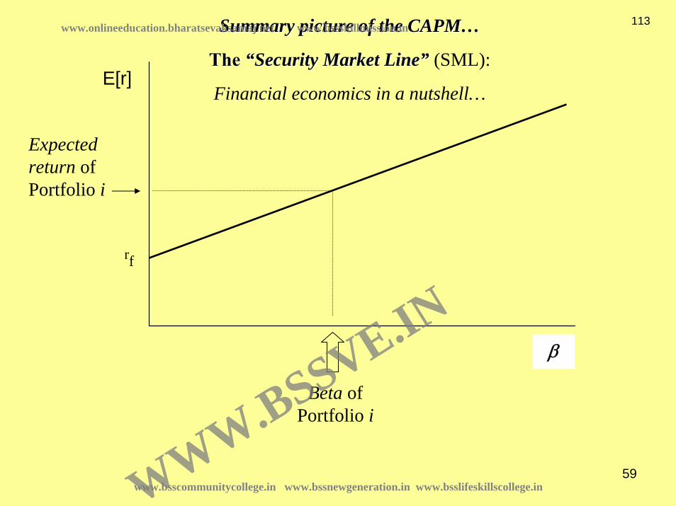
59
rf
β
E[r]
Beta of Portfolio i
Expected return of Portfolio i
Summary picture of the CAPMSummary picture of the CAPM……
The The ““Security Market LineSecurity Market Line”” (SML):
Financial economics in a nutshell…
www.bsscommunitycollege.in www.bssnewgeneration.in www.bsslifeskillscollege.in
113www.onlineeducation.bharatsevaksamaj.net www.bssskillmission.in
WWW.BSSVE.IN

60
THE CAPM IS OBVIOUSLY A SIMPLIFICATION (of reality)… (Yes, I know that markets are not really perfectly efficient. I know we don’t all have the same expectations. I know we do not all really hold the same portfolios.) BUT IT IS A POWERFUL AND WIDELY-USED MODEL. IT CAPTURES AN IMPORTANT PART OF THE ESSENCE OF REALITY ABOUT ASSET MARKET PRICING…
www.bsscommunitycollege.in www.bssnewgeneration.in www.bsslifeskillscollege.in
114www.onlineeducation.bharatsevaksamaj.net www.bssskillmission.in
WWW.BSSVE.IN

61
22.1.6 Strengths and Weaknesses in the Basic CAPM22.1.6 Strengths and Weaknesses in the Basic CAPM
Strengths:• Useful as normative (what should be) prescription (it makes sense).• As positive (what is) description the classical (original) single-factor CAPM has some value (especially at broad-brush level, as we’ll see later).• Provides basic and elegant intuition that may at least partly explain why more complex models work better (e.g., maybe “Fama-French factors” proxy for types of systematic risk not quantified by beta).
Weaknesses:• Without “enhancements” (e.g., Fama-French factors), the basic single-factor CAPM is a pretty incomplete model of the expected returns of specific portfolios within an asset class.
www.bsscommunitycollege.in www.bssnewgeneration.in www.bsslifeskillscollege.in
115www.onlineeducation.bharatsevaksamaj.net www.bssskillmission.in
WWW.BSSVE.IN

62
Section 22.2Section 22.2
Applying the CAPM at the Asset Class LevelApplying the CAPM at the Asset Class Level
The basic single-factor CAPM does a pretty decent job of explaining the expected return to the real estate asset class as a whole, provided you:
• Correct the real estate returns for appraisal smoothing and lagging, and;
• Define the “market portfolio” to include all investible wealth, including real estate.
For the former purpose, you can accumulate the contemporaneous plus lagged covariances between the real estate index and the market portfolio. Or you can use “unsmoothed” or transactions-based real estate indexes.
For the latter, you can define the market portfolio as a stylized “National Wealth Portfolio” consisting of one-third shares each of stocks, bonds, and real estate.
www.bsscommunitycollege.in www.bssnewgeneration.in www.bsslifeskillscollege.in
116www.onlineeducation.bharatsevaksamaj.net www.bssskillmission.in
WWW.BSSVE.IN

63
22.2.2 22.2.2 Applying the Basic CAPMApplying the Basic CAPM ACROSSACROSS asset classesasset classes
Correcting for smoothing, and defining betawrt National Wealth…
““CAPM CAPM works.works.””
SMALL STKs
S&P500
NAREIT
L T Bond
CMortes
IT BandCMBS
NCREIF
0.00.0
0.5
1.0
1.5
2.0
2.5
3.0
0.2 0.4 0.6 0.8 1.0 1.2 1.4 1.6 1.8 2.0
Avg
RP
over
T-b
ills (
%Q
tr)
Beta wrt NWP
Empirical Security Market Line and Historical Risk & Return on Eight U.S. Domestic Asset Classes Based on Quarterly Returns 1980-2004 (95 obs) "NWP" = 1/3 Stocks + 1/3 Bonds + 1/3 Real Estate
Regression: R2 = 93%; Intercept = 0.17% (t-stat = 1.2); Slope = 1.24 (t-stat = 10.0).
Figure by MIT OCW.www.bsscommunitycollege.in www.bssnewgeneration.in www.bsslifeskillscollege.in
117www.onlineeducation.bharatsevaksamaj.net www.bssskillmission.in
WWW.BSSVE.IN

64
Fama-French: CAPM by itself doesn’t work very well within the stock market:
22.3.122.3.1The simple 1-factor CAPM has trouble empirically within asset classes.
Enhance the basic model with additional factors that are more “tangible”than beta: (i) Stock’s Size (mkt cap), & (ii) Stock’s Book/Market Value
Ratio. The market apparently associates these with “risk”.
1 (Lowest B/M)
2345
6
78
9
10 (Highest B/M)
Average returnspredicted bythe CAPM
Beta0.7 0.8 0.9 1.1 1.21
9
10
11
12
13
14
15
16
17Av
erag
e an
nual
ized
mon
thly
retu
rn (%
)
Average Annualized Monthly Return versus Beta for Value Weight Portfolios Formed on B/M, 1963-2003
Figure by MIT OCW.
www.bsscommunitycollege.in www.bssnewgeneration.in www.bsslifeskillscollege.in
118www.onlineeducation.bharatsevaksamaj.net www.bssskillmission.in
WWW.BSSVE.IN

65
Similarly, within the real estate asset class, beta does not explain the dispersion in long-run average total returns (nor does simple volatility).
The market pays more attention to tangible aspects of properties, most notably property size and quality (whether a property is “institutional” or
not), and property usage type (e.g., office bldgs are “lower risk”?)
Aver
age
Exce
ss R
etur
ns p
er a
nnum
(ove
r T-b
ills)
NCREIF Division/Type Portfolios:Returns vs National Wealth Portfolio Factor Risk
0.0 0.5 1.0 1.5 2.0 2.5
-4%
-2%
0%
2%
4%
6%
8%
Beta with respect to National Wealth Portfolio, defined as equalone-third shares of stocks, bonds, and real estate.
Figure by MIT OCW.
www.bsscommunitycollege.in www.bssnewgeneration.in www.bsslifeskillscollege.in
119www.onlineeducation.bharatsevaksamaj.net www.bssskillmission.in
WWW.BSSVE.IN

66
Size - Total Return vs Beta (NCREIF)
R&D S
R&D M
R&D L
Apt S
Apt M
Apt L
Whr S
Whr MWhr L
CBD S
CBD M
CBD L
Sub S
Sub M
Sub L
Ret S
Ret MRet L
0.00%
2.00%
4.00%
6.00%
8.00%
10.00%
12.00%
14.00%
0.00 0.20 0.40 0.60 0.80 1.00 1.20 1.40 1.60 1.80 2.00 Beta (NCREIF)
Tota
l Ret
urn
Apts
Retail
Warehouses
R&D Space
Office
NCREIF portfolio avg returns and beta wrt NPI (1984-2003) by property size and type
The market pays more attention to tangible aspects of propertiesThe market pays more attention to tangible aspects of properties, most , most notably property size and quality (whether a property is notably property size and quality (whether a property is ““institutionalinstitutional””or not), and property usage type (e.g., office or not), and property usage type (e.g., office bldgsbldgs are are ““lower risklower risk””?)?)
www.bsscommunitycollege.in www.bssnewgeneration.in www.bsslifeskillscollege.in
120www.onlineeducation.bharatsevaksamaj.net www.bssskillmission.in
WWW.BSSVE.IN

67
The Capital Market does perceive (and price) risk differences The Capital Market does perceive (and price) risk differences ACROSSACROSS asset classes . . .asset classes . . .
National Wealth BETABETA
Pub.EqPub.Eq
Pub.DbPub.Db
Pri.DbPri.Db
Pri.EqPri.Eq
Real estate based asset classes: Property, Mortgages, CMBS, Real estate based asset classes: Property, Mortgages, CMBS, REITsREITs……
www.bsscommunitycollege.in www.bssnewgeneration.in www.bsslifeskillscollege.in
121www.onlineeducation.bharatsevaksamaj.net www.bssskillmission.in
WWW.BSSVE.IN

68
A CAPMA CAPM--based method to adjust investment performance for based method to adjust investment performance for risk: The risk: The TreynorTreynor RatioRatio......
Avg. Excess Return
Beta
SML
1
rM - rf
0
ri - rf
iβ
TRi
Based on ““Risk BenchmarkRisk Benchmark””www.bsscommunitycollege.in www.bssnewgeneration.in www.bsslifeskillscollege.in
122www.onlineeducation.bharatsevaksamaj.net www.bssskillmission.in
WWW.BSSVE.IN

69
The The TreynorTreynor Ratio Ratio (or something like it) could perhaps be (or something like it) could perhaps be applied to managers (portfolios) spanning the major asset applied to managers (portfolios) spanning the major asset classes...classes...
Avg. Excess Return
Beta
SML
1
rM - rf
0
ri - rf
iβ
TRi
www.bsscommunitycollege.in www.bssnewgeneration.in www.bsslifeskillscollege.in
123www.onlineeducation.bharatsevaksamaj.net www.bssskillmission.in
WWW.BSSVE.IN

70
The The Beta Beta can be estimated based on the can be estimated based on the ““National Wealth National Wealth PortfolioPortfolio”” (( = (1/3)Stocks + (1/3)Bonds + (1/3)RE = (1/3)Stocks + (1/3)Bonds + (1/3)RE ) as the ) as the mixedmixed--asset asset ““Risk BenchmarkRisk Benchmark””. . .. . .
Beta
SML
1
rM - rf
0
ri - rf
iβ
TRi
Based on ““National Wealth PortfolioNational Wealth Portfolio””www.bsscommunitycollege.in www.bssnewgeneration.in www.bsslifeskillscollege.in
124www.onlineeducation.bharatsevaksamaj.net www.bssskillmission.in
WWW.BSSVE.IN

71
22.3.2: Go back to the 22.3.2: Go back to the within the private real estate asset classwithin the private real estate asset class level of level of application of the CAPMapplication of the CAPM……
Recall that we see little ability to systematically or rigorousRecall that we see little ability to systematically or rigorously distinguish ly distinguish between the risk and return expectations for different market sebetween the risk and return expectations for different market segments gments withinwithin the asset class (e.g., Denver shopping the asset class (e.g., Denver shopping ctrsctrs vsvs Boston office Boston office bldgsbldgs):):
Aver
age
Exce
ss R
etur
ns p
er a
nnum
(ove
r T-b
ills)
NCREIF Division/Type Portfolios:Returns vs National Wealth Portfolio Factor Risk
0.0 0.5 1.0 1.5 2.0 2.5
-4%
-2%
0%
2%
4%
6%
8%
Beta with respect to National Wealth Portfolio, defined as equalone-third shares of stocks, bonds, and real estate.
Figure by MIT OCW.www.bsscommunitycollege.in www.bssnewgeneration.in www.bsslifeskillscollege.in
125www.onlineeducation.bharatsevaksamaj.net www.bssskillmission.in
WWW.BSSVE.IN

72
This holds implications for portfolioThis holds implications for portfolio--level tactical investment policy:level tactical investment policy:•• If all If all mktmkt segments effectively present the same investment risk, then thosegments effectively present the same investment risk, then those that se that present the highest expected returns automatically look like present the highest expected returns automatically look like ““good investmentsgood investments””(bargains) from a risk(bargains) from a risk--adjusted ex ante return perspective.adjusted ex ante return perspective.
•• Search for markets where the combination of current asset yieldSearch for markets where the combination of current asset yields (cap rates, s (cap rates, ““yy””) ) and rental growth prospects (and rental growth prospects (““gg””) present higher expected total returns () present higher expected total returns (ErEr = y + = y + EgEg).).
Figure by MIT OCW.
Aver
age
Exce
ss R
etur
ns p
er a
nnum
(ove
r T-b
ills)
NCREIF Division/Type Portfolios:Returns vs National Wealth Portfolio Factor Risk
0.0 0.5 1.0 1.5 2.0 2.5
-4%
-2%
0%
2%
4%
6%
8%
Beta with respect to National Wealth Portfolio, defined as equalone-third shares of stocks, bonds, and real estate.
www.bsscommunitycollege.in www.bssnewgeneration.in www.bsslifeskillscollege.in
126www.onlineeducation.bharatsevaksamaj.net www.bssskillmission.in
WWW.BSSVE.IN

73
Summarizing Chapter 22: Summarizing Chapter 22: Equilibrium Asset Price Equilibrium Asset Price ModellingModelling & Real Estate& Real Estate•• Like the MPT on which it is based, equilibrium asset price modelLike the MPT on which it is based, equilibrium asset price modeling (the ing (the CAPM in particular) has substantial relevance and applicability CAPM in particular) has substantial relevance and applicability to real estate to real estate when applied at the broadwhen applied at the broad--brush level ( brush level ( across asset classesacross asset classes ).).•• At the property level (At the property level (unleveredunlevered), real estate in general tends to be a low), real estate in general tends to be a low--beta, beta, lowlow--return asset class in equilibrium, but certainly not return asset class in equilibrium, but certainly not risklessriskless, requiring (and , requiring (and providing) some positive risk premium (ex ante).providing) some positive risk premium (ex ante).•• CAPM type models can provide some guidance regarding the relatiCAPM type models can provide some guidance regarding the relative pricing ve pricing of real estate as compared to other asset classes (of real estate as compared to other asset classes (““Should it currently be overShould it currently be over--weighted or underweighted or under--weighted?weighted?””), and), and……•• CAPMCAPM--based riskbased risk--adjusted return measures (such as the adjusted return measures (such as the TreynorTreynor Ratio) may Ratio) may provide a basis for helping to judge the performance of multiprovide a basis for helping to judge the performance of multi--assetasset--class class investment managers (who can allocate across asset classes).*investment managers (who can allocate across asset classes).*•• WithinWithin the private real estate asset class, the CAPM is less effectivethe private real estate asset class, the CAPM is less effective at at distinguishing between the relative levels of risk among real esdistinguishing between the relative levels of risk among real estate market tate market segments, implying (within the state of current knowledge) a gensegments, implying (within the state of current knowledge) a generally erally flat flat security market linesecurity market line..•• This holds implications for tactical portfolio investment reseaThis holds implications for tactical portfolio investment research & policy rch & policy within the private real estate asset class:within the private real estate asset class: Search for market segments with a Search for market segments with a combination of high asset yields and high rental growth opportuncombination of high asset yields and high rental growth opportunities: Such ities: Such apparent apparent ““bargainsbargains”” present favorable riskpresent favorable risk--adjusted ex ante returns.adjusted ex ante returns.
www.bsscommunitycollege.in www.bssnewgeneration.in www.bsslifeskillscollege.in
127www.onlineeducation.bharatsevaksamaj.net www.bssskillmission.in
WWW.BSSVE.IN

1
Chapter 23:Chapter 23:
Real Estate Investment Trusts Real Estate Investment Trusts ((REITsREITs))
Also including a review of Ch 12 Section 12.3:
“Dueling Asset Markets”
www.bsscommunitycollege.in www.bssnewgeneration.in www.bsslifeskillscollege.in
128www.onlineeducation.bharatsevaksamaj.net www.bssskillmission.in
WWW.BSSVE.IN

2
““MacroMacro--level valuationlevel valuation”” Valuation of aggregates of numerous Valuation of aggregates of numerous individual properties, e.g., portfolios, indices, funds, individual properties, e.g., portfolios, indices, funds, REITsREITs……
The The spectrumspectrum of macroof macro--level R.E. equity investment entities:level R.E. equity investment entities:
StaticPortfolios,Indices
FundsUnit TrustsLPs REITsREITs
REOCs
Valuation issue:Valuation issue:•• Static portfolios (private assets) Static portfolios (private assets) Value Value estimation (measurement).estimation (measurement).•• REITs (publiclyREITs (publicly--traded assets) traded assets) Value Value determination (causal).determination (causal).
EntityEntity--Level ValuationLevel ValuationPropertyProperty--Level ValuationLevel Valuation
Direct, passive investment in propertyIndirect investment in property,
actively-managed entities.
www.bsscommunitycollege.in www.bssnewgeneration.in www.bsslifeskillscollege.in
129www.onlineeducation.bharatsevaksamaj.net www.bssskillmission.in
WWW.BSSVE.IN

3
What are Real Estate Investment Trusts?What are Real Estate Investment Trusts?
• Operating companies that own, develop and manage commercial real estate
• Chartered as a corporation or business trust
• Elective choice under tax code creates pass-through of income
• Revenue must primarily come from real estate investments
• Required to distribute at least 90 percent of their taxable income
• Taxation of income is passed through to shareholder level
www.bsscommunitycollege.in www.bssnewgeneration.in www.bsslifeskillscollege.in
130www.onlineeducation.bharatsevaksamaj.net www.bssskillmission.in
WWW.BSSVE.IN

4
What Makes a REIT Different?What Makes a REIT Different?
• 75 percent of assets must be invested in:• Equity ownership of real property• Mortgages • Other REIT shares• Government securities and cash
• 75 percent of revenue must come from:• Rents from real property • Mortgage interest• Gains from sales of real property
www.bsscommunitycollege.in www.bssnewgeneration.in www.bsslifeskillscollege.in
131www.onlineeducation.bharatsevaksamaj.net www.bssskillmission.in
WWW.BSSVE.IN

5
Large REITs are actively-managed, vertically integrated firms providing commercial real estate goods and services for their “customers” (tenants & users of space). “Vertical integration”:
• Land acquisition/holding
• Development
• Ownership o Financial capital provision o Asset (portfolio) management
• Operation
o Asset management (franchise value, synergy)o Property management
• Tenant services
www.bsscommunitycollege.in www.bssnewgeneration.in www.bsslifeskillscollege.in
132www.onlineeducation.bharatsevaksamaj.net www.bssskillmission.in
WWW.BSSVE.IN

6
PublicPublic REITsREITs as a Core Asset Classas a Core Asset Class
• REITs = Real Estate Stocks• REITs have distinct investment performance
characteristics• REIT returns are influenced by:
• Real estate fundamentals• Equity market valuations
• Real estate market supply and demand determine occupancy and rental growth
• Equity market assesses risk and prices cash flow
www.bsscommunitycollege.in www.bssnewgeneration.in www.bsslifeskillscollege.in
133www.onlineeducation.bharatsevaksamaj.net www.bssskillmission.in
WWW.BSSVE.IN

7
REITsREITs in a mixed asset in a mixed asset portfolioportfolio……
“REITs smell like real estate, look like bonds and walk like equity”
Greg Whyte, Analyst, Morgan Stanley
www.bsscommunitycollege.in www.bssnewgeneration.in www.bsslifeskillscollege.in
134www.onlineeducation.bharatsevaksamaj.net www.bssskillmission.in
WWW.BSSVE.IN

8
Comparative Total Return Investment Performance:Equity Real Estate (Public and Private) versus Stocks
-30%
-20%
-10%
0%
10%
20%
30%
40%
50%
60%
1993 1994 1995 1996 1997 1998 1999 2000 2001 2002 2003 2004 2005 2006(1Q)
NAREIT S&P500Russell 2000 NCREIF Property Index
Source: National Association of Real Estate Investment Trusts (NAREIT).
www.bsscommunitycollege.in www.bssnewgeneration.in www.bsslifeskillscollege.in
135www.onlineeducation.bharatsevaksamaj.net www.bssskillmission.in
WWW.BSSVE.IN

9
Comparative Total Return Investment Performance:REITs versus Small Cap Growth and Value Stocks
-40%
-30%
-20%
-10%
0%
10%
20%
30%
40%
50%
60%
1993 1994 1995 1996 1997 1998 1999 2000 2001 2002 2003 2004 2005 2006(1Q)
NAREIT Russell 2000 Growth Russell 2000 Value
Source: NAREIT
www.bsscommunitycollege.in www.bssnewgeneration.in www.bsslifeskillscollege.in
136www.onlineeducation.bharatsevaksamaj.net www.bssskillmission.in
WWW.BSSVE.IN
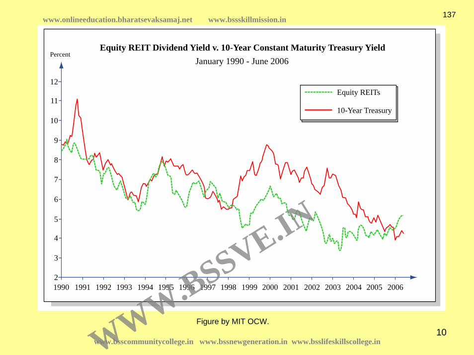
10
Percent
Equity REITs
10-Year Treasury
12
11
10
9
8
7
6
5
4
3
21990 1991 1992 1993 1994 1995 1996 1997 1998 1999 2000 2001 2002 2003 2004 2005 2006
Equity REIT Dividend Yield v. 10-Year Constant Maturity Treasury YieldJanuary 1990 - June 2006
Figure by MIT OCW.
www.bsscommunitycollege.in www.bssnewgeneration.in www.bsslifeskillscollege.in
137www.onlineeducation.bharatsevaksamaj.net www.bssskillmission.in
WWW.BSSVE.IN

11
PublicPublic REITsREITs are are ……
Like typical industrial/service/information companies traded on Like typical industrial/service/information companies traded on the stock exchanges, the stock exchanges, except:except:
•• Exempt from corporate income taxExempt from corporate income tax
•• Restricted to real estate investment related activitiesRestricted to real estate investment related activities
•• Restrictions on Restrictions on ““merchant buildingmerchant building””
•• Must pay out 90% of earnings in dividendsMust pay out 90% of earnings in dividends
So So REITsREITs are are ““different animalsdifferent animals”” –– somewhat passive somewhat passive (compared to other stocks), (compared to other stocks), ““pure playspure plays”” (in real estate).(in real estate).
www.bsscommunitycollege.in www.bssnewgeneration.in www.bsslifeskillscollege.in
138www.onlineeducation.bharatsevaksamaj.net www.bssskillmission.in
WWW.BSSVE.IN

12
REIT InvestorsREIT Investors……REIT Investors (early 2000s)
Insiders10%
REIT Mut Fds10%
Pension Funds10%
International5%
Retail investors (individ)
35%
Mut Fds30%
Yield-orientedValue-orientedSmall-Mid cap
e.g., Green StreetCohen-SteersVanguardEtc…
Recall:Recall: Different types of investors have different Different types of investors have different objectives, constraints, objectives, constraints, concerns, horizons, incomeconcerns, horizons, income--vsvs--growth preferences, risk preferences, etcgrowth preferences, risk preferences, etc……
www.bsscommunitycollege.in www.bssnewgeneration.in www.bsslifeskillscollege.in
139www.onlineeducation.bharatsevaksamaj.net www.bssskillmission.in
WWW.BSSVE.IN

13
23.1.1 Tax Status, Regulatory Constraints and FFOREITsREITs are are exempt from corporate income taxexempt from corporate income tax::
Original intent of 1960 REIT Act was to create a Original intent of 1960 REIT Act was to create a ““mutual fundmutual fund”” type type vehicle to allow small investors to invest in commercial real esvehicle to allow small investors to invest in commercial real estate. tate. (Mutual funds pay no taxes, but pass through tax obligations to (Mutual funds pay no taxes, but pass through tax obligations to investors on dividends and CG realized in the fund each year.) Tinvestors on dividends and CG realized in the fund each year.) To o implement the spirit of this law, implement the spirit of this law, REITsREITs must be:must be:
•• Passive Passive ““passpass--throughthrough”” type vehicles similar to mutual funds;type vehicles similar to mutual funds;
•• Confined to Confined to ““pure playspure plays”” in real estate investment;in real estate investment;
•• Required to maintain broadlyRequired to maintain broadly--dispersed ownership (many dispersed ownership (many investors).investors).
Some of these requirements have been relaxed over the years, butSome of these requirements have been relaxed over the years, but several several constraints are currently applied to constraints are currently applied to REITsREITs (and are likely to (and are likely to remain)remain)……
23.1 REIT Structure and Market Evolution23.1 REIT Structure and Market Evolution
www.bsscommunitycollege.in www.bssnewgeneration.in www.bsslifeskillscollege.in
140www.onlineeducation.bharatsevaksamaj.net www.bssskillmission.in
WWW.BSSVE.IN

14
1) 1) ““Five or Fewer RuleFive or Fewer Rule””.. A REIT cannot be a closely held corporation. No five or fewer individuals (and certain trusts) may own more than 50% of the REIT's stock, and there must be at least 100 different shareholders. [Ownership Test]
2) 2) ““Real Estate Pure PlayReal Estate Pure Play””.. 75% or more of the REITs total assets must be real estate, mortgages, cash, or federal government securities, and 75% or more of the REIT’s yearly gross income must be derived directly or indirectly from real property (including mortgages, partnerships and other REITs). [Asset Test]
3) 3) ““Passive Investment Entity RequirementPassive Investment Entity Requirement””.. REITs must derive their income from primarily passive sources like rents and mortgage interest, as distinct from short-term trading or sale of property assets. They cannot use their tax status to shield non-real-estate income from corporate taxation. A REIT is subject to a tax of 100%100% on net income from "prohibited transactions", such as the sale or other disposition of property held primarily for sale in the ordinary course of its trade or business. However, if the REIT sells property it has held for at least 4 yearsheld for at least 4 years and the aggregate adjusted basis of the property sold does not exceed 10%10% of the aggregate basis of all assets of the REIT as of the beginning of the year, then no prohibited transaction is deemed to have occurred. [Income Test]
4) 4) ““Earnings Payout RequirementEarnings Payout Requirement””.. 90% or more of the REIT’s annual taxable income must be distributed to shareholders as dividends each year. (Shareholders will then pay ordinary income tax on the earnings in their personal taxes.) [Distribution Test]
Major REIT constraints required to maintain taxMajor REIT constraints required to maintain tax--exempt status:exempt status:
www.bsscommunitycollege.in www.bssnewgeneration.in www.bsslifeskillscollege.in
141www.onlineeducation.bharatsevaksamaj.net www.bssskillmission.in
WWW.BSSVE.IN

15
How binding is the 90% payout constraint? . . .How binding is the 90% payout constraint? . . .The 90% earnings payout requirement could force The 90% earnings payout requirement could force REITsREITs to rely more to rely more heavily on heavily on external sources of capitalexternal sources of capital (e.g., stock (e.g., stock mktmkt, bond , bond mktmkt, , mortgages) than other corporations.mortgages) than other corporations.
But in fact, this constraint has not usually been binding:But in fact, this constraint has not usually been binding:•• Typical REIT pays out more than the minimum requirement.Typical REIT pays out more than the minimum requirement.
This is because:This is because:•• Real estate is a capital intensive business investing in Real estate is a capital intensive business investing in ““cash cash cowscows””, not a growth industry demanding constant cash feeding., not a growth industry demanding constant cash feeding.•• IRS depreciation rules allow property assets to be depreciated IRS depreciation rules allow property assets to be depreciated even though nominal values and cash flow generation typically doeven though nominal values and cash flow generation typically donot decline, hence, not decline, hence, depreciation expenses shelterdepreciation expenses shelter much cash flow much cash flow (reducing (reducing taxabletaxable income, hence reducing the payout income, hence reducing the payout requirement).requirement).
During the 1990s the thenDuring the 1990s the then--requirement of 95% earnings payout requirement of 95% earnings payout typically equated to only about 60% of REIT operational cash flotypically equated to only about 60% of REIT operational cash flow, w, and the average REIT dividend payout was about 65% of such CF.and the average REIT dividend payout was about 65% of such CF.
www.bsscommunitycollege.in www.bssnewgeneration.in www.bsslifeskillscollege.in
142www.onlineeducation.bharatsevaksamaj.net www.bssskillmission.in
WWW.BSSVE.IN

16
EBIDTA $100- Interest 20- Depreciation 30
= GAAP Net Income $50-------------------Dividends Paid $54.25
How binding is the 90% payout constraint? How binding is the 90% payout constraint? A first look at FFO FFO at a basic level at a basic level ……
How can the REIT pay more in dividends than it receives in income?
•GAAP NI represents accounting earningsaccounting earnings not cash flowcash flow
•Funds from Operation (FFO) = GAAP NI + Depreciation
FFO = $80 & Div/FFO = 54.25/80 = 68% << 90%
$54.25 > 90% * $50 = $45.Hence REIT “passes”Distribution Test.
www.bsscommunitycollege.in www.bssnewgeneration.in www.bsslifeskillscollege.in
143www.onlineeducation.bharatsevaksamaj.net www.bssskillmission.in
WWW.BSSVE.IN

17www.bsscommunitycollege.in www.bssnewgeneration.in www.bsslifeskillscollege.in
144www.onlineeducation.bharatsevaksamaj.net www.bssskillmission.in
WWW.BSSVE.IN

18
There have been some significant relaxations of REIT There have been some significant relaxations of REIT constraints, most notably:constraints, most notably:
•• 1986: 1986: REITsREITs permitted to permitted to ““self manageself manage””, no longer have to hire , no longer have to hire an external manager.an external manager.
•• This permits This permits REITsREITs to be much more to be much more ““activeactive””, integrated , integrated corporations, similar to typical industrial firms (only still sucorporations, similar to typical industrial firms (only still subject bject to the previouslyto the previously--noted constraints).noted constraints).
•• 1993: 1993: REITsREITs permitted to permitted to ““look throughlook through”” a pension fund to count a pension fund to count it as a number of investors equal to its members (avoids it as a number of investors equal to its members (avoids Five or Five or FewerFewer RuleRule for pension fund investment in for pension fund investment in REITsREITs).).
•• 1999: 1999: REITsREITs permitted to engage in nonpermitted to engage in non--REIT type activity via REIT type activity via Taxable REIT SubsidiariesTaxable REIT Subsidiaries (TRS), in which the subsidiary is subject (TRS), in which the subsidiary is subject to corporate income tax (e.g., 3to corporate income tax (e.g., 3rdrd--party property management, party property management, brokerage, property trading).brokerage, property trading).
www.bsscommunitycollege.in www.bssnewgeneration.in www.bsslifeskillscollege.in
145www.onlineeducation.bharatsevaksamaj.net www.bssskillmission.in
WWW.BSSVE.IN

19
•• Nevertheless, the REIT restrictions (not just the 90% payout rule, but other constraints previously noted as well), do have some limiting effect on REIT operations, … at least for some REITs at some times.
• These restrictions may provide some reason, in specific instances, why a REIT’s stock market valuation might be less than the NAV of the property assets it owns.
• And to avoid these constraints is the reason why many real estate firms (some publicly-traded) have elected to be “C-corporations”subject to corporate income tax.
• Such firms are called “REOCsREOCs” (Real Estate Operating Companies).
• Obviously, the “merchant building” firms, such as the major publicly-traded tract housing developers, are all REOCs.
www.bsscommunitycollege.in www.bssnewgeneration.in www.bsslifeskillscollege.in
146www.onlineeducation.bharatsevaksamaj.net www.bssskillmission.in
WWW.BSSVE.IN
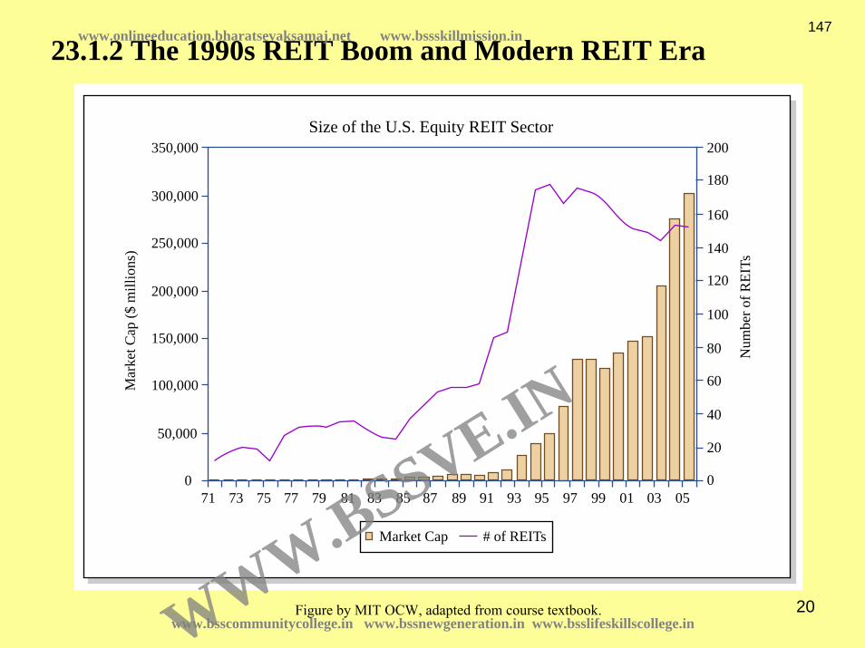
20
23.1.2 The 1990s REIT Boom and Modern REIT Era
350,000
300,000
250,000
200,000
150,000
100,000
50,000
071 73 75 77 79 81 83 85 87 89 91 93 95 97 99 01 03 05
0
20
40
60
80
100
120
140
160
180
200Size of the U.S. Equity REIT Sector
Num
ber o
f REI
Ts
Mar
ket C
ap ($
mill
ions
)
Market Cap # of REITs
Figure by MIT OCW, adapted from course textbook.www.bsscommunitycollege.in www.bssnewgeneration.in www.bsslifeskillscollege.in
147www.onlineeducation.bharatsevaksamaj.net www.bssskillmission.in
WWW.BSSVE.IN

21
30,000
25,000
20,000
15,000
10,000
5,000
090 91 92 93 94 95 96 97 98 99 00 01 02 03 04 05
Mill
ions
of D
olla
rs R
aise
d
IPOs SEOs
Equity Capital Raised in Initial Public Offerings (IPOs) and Secondary Offerings(SEOs), U.S. REIT Sector
Figure by MIT OCW, adapted from course textbook.
www.bsscommunitycollege.in www.bssnewgeneration.in www.bsslifeskillscollege.in
148www.onlineeducation.bharatsevaksamaj.net www.bssskillmission.in
WWW.BSSVE.IN

22
1992 1993 1994 1995 1996 1997 1998 1999 2000 2001 2002 2003 2004 2005 2006
12
10
8
6
4
2
0
14
16
18
Securities Offerings by REITs
Billions of Dollars
(Quarterly 1992:Q1-2006:Q2)
Debt
Equity
Figure by MIT OCW.
www.bsscommunitycollege.in www.bssnewgeneration.in www.bsslifeskillscollege.in
149www.onlineeducation.bharatsevaksamaj.net www.bssskillmission.in
WWW.BSSVE.IN

23
1992 1993 1994 1995 1996 1997 1998 1999 2000 2001 2002 2003 2004 2005 2006
10
0
5
15
20
25
30
Property Acquisition by REITs(Quarterly 1992:Q1-2006:Q4)
Billions of Dollars
Figure by MIT OCW.
www.bsscommunitycollege.in www.bssnewgeneration.in www.bsslifeskillscollege.in
150www.onlineeducation.bharatsevaksamaj.net www.bssskillmission.in
WWW.BSSVE.IN

24www.bsscommunitycollege.in www.bssnewgeneration.in www.bsslifeskillscollege.in
151www.onlineeducation.bharatsevaksamaj.net www.bssskillmission.in
WWW.BSSVE.IN

25
REIT Membership in the S&P 500 Index
AIMCO AIV 3/13/2003 Archstone-Smith ASN 12/17/2004 Boston Properties BXP 3/31/2006 Equity Office EOP 10/1/2001 Equity Residential EQR 11/1/2001 Kimco Realty KIM 4/3/2006 Plum Creek Timber PCL 1/16/2002 ProLogis PLD 7/16/2003 Public Storage, Inc. PSA 8/18/2005 Simon Property SPG 6/25/2002 Vornado Realty Trust VNO 8/11/2005
In the fall of 2001 … REITs finally gain some respect!
www.bsscommunitycollege.in www.bssnewgeneration.in www.bsslifeskillscollege.in
152www.onlineeducation.bharatsevaksamaj.net www.bssskillmission.in
WWW.BSSVE.IN
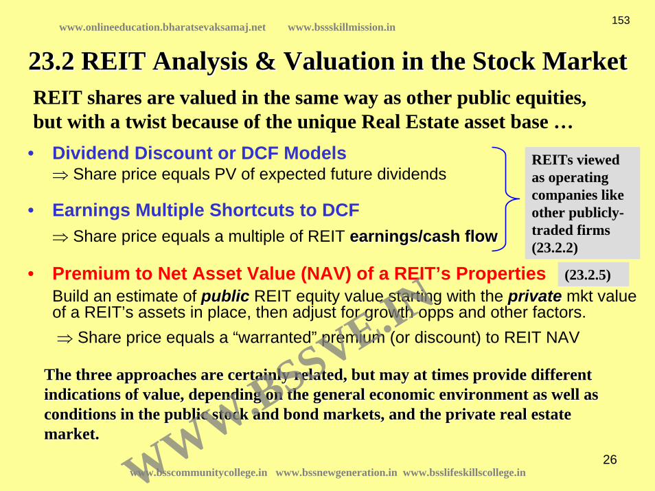
26
23.2 REIT Analysis & Valuation in the Stock Market23.2 REIT Analysis & Valuation in the Stock Market
• Dividend Discount or DCF Models⇒ Share price equals PV of expected future dividends
• Earnings Multiple Shortcuts to DCF⇒ Share price equals a multiple of REIT earnings/cash flowearnings/cash flow
• Premium to Net Asset Value (NAV) of a REIT’s PropertiesBuild an estimate of publicpublic REIT equity value starting with the privateprivate mkt value of a REIT’s assets in place, then adjust for growth opps and other factors.⇒ Share price equals a “warranted” premium (or discount) to REIT NAV
REIT shares are valued in the same way as other public equities,but with a twist because of the unique Real Estate asset base …
REITs viewed as operating companies like other publicly-traded firms (23.2.2)
The three approaches are certainly related, but may at times proThe three approaches are certainly related, but may at times provide different vide different indications of value, depending on the general economic environmindications of value, depending on the general economic environment as well as ent as well as conditions in the public stock and bond markets, and the privateconditions in the public stock and bond markets, and the private real estate real estate market.market.
(23.2.5)
www.bsscommunitycollege.in www.bssnewgeneration.in www.bsslifeskillscollege.in
153www.onlineeducation.bharatsevaksamaj.net www.bssskillmission.in
WWW.BSSVE.IN

27
23.2.1 More on REIT Earnings Measures23.2.1 More on REIT Earnings Measures
The Problem:The Problem:How to compare REIT earnings with those of other corporations How to compare REIT earnings with those of other corporations (e.g., so as to compare share (e.g., so as to compare share price/earningsprice/earnings multiples on an multiples on an ““apples apples vsvs applesapples”” basis.basis.•• Real estate investment & ownership (the Real estate investment & ownership (the ““REIT businessREIT business””) is ) is very very capital intensivecapital intensive::•• REITsREITs have abnormally high have abnormally high depreciation expensesdepreciation expenses, which reduce , which reduce ““official earningsofficial earnings”” (GAAP net income)(GAAP net income), the standard measure of , the standard measure of corporate earnings on Wall Street.corporate earnings on Wall Street.•• Yet REIT assets do not actually depreciate in the sense that Yet REIT assets do not actually depreciate in the sense that ““samesame--storestore”” property cash flows and values typically do not decline in nomiproperty cash flows and values typically do not decline in nominal nal terms (because the terms (because the real depreciationreal depreciation rate in property is typically matched rate in property is typically matched or even exceeded by the general monetaryor even exceeded by the general monetary inflationinflation rate).rate).
Hence (so the argument goes):Hence (so the argument goes):GAAP earnings donGAAP earnings don’’t present a t present a ““fairfair”” or or ““accurateaccurate”” measure of measure of
REIT earnings.REIT earnings.www.bsscommunitycollege.in www.bssnewgeneration.in www.bsslifeskillscollege.in
154www.onlineeducation.bharatsevaksamaj.net www.bssskillmission.in
WWW.BSSVE.IN

28
In the early 1990s, the REIT industry (through NAREIT) came up wIn the early 1990s, the REIT industry (through NAREIT) came up with ith an an alternative measure of earnings alternative measure of earnings that the industry tried to promulgate that the industry tried to promulgate as a substitute for GAAP net income for the REIT industry:as a substitute for GAAP net income for the REIT industry:
““Funds From OperationsFunds From Operations””FFOFFO
FFO (“Funds From Operations”)
Start with GAAP net income, GAAP net income, then then
Add back: Real property depreciation expense.
Add back: Preferred stock dividends and distributions to OP unit- holders.
Deduct: Net gains from property sales & extraordinary items.
FFO FFO ≈≈ Aggregate (i.e. firm level) NOI Aggregate (i.e. firm level) NOI -- interestinterest
www.bsscommunitycollege.in www.bssnewgeneration.in www.bsslifeskillscollege.in
155www.onlineeducation.bharatsevaksamaj.net www.bssskillmission.in
WWW.BSSVE.IN

29
This was further supplemented by another measure that more closeThis was further supplemented by another measure that more closely ly reflected cash flow actually available for external distributionreflected cash flow actually available for external distribution: :
““Adjusted Funds From OperationsAdjusted Funds From Operations””AFFOAFFO
AFFO (“Adjusted Funds from Operation”) – sim to & smtms aka “Funds Available for Distritution” (FAD*)
Start with FFO, then:
Deduct: Recurring capital improvement expenditures (CI).
Adjust for: Straight-line rents.
Deduct: Amortization of debt principle (AMORT).
Terminology Alert!Terminology Alert!In common parlance it is often not clear exactly what measure isIn common parlance it is often not clear exactly what measure is being being
referred to when people use the terms referred to when people use the terms ““FFOFFO”” and and ““AFFOAFFO””..
AFFO AFFO ≈≈ Aggregate (i.e. firm level) EBTCFAggregate (i.e. firm level) EBTCF Less entity level overhead
www.bsscommunitycollege.in www.bssnewgeneration.in www.bsslifeskillscollege.in
156www.onlineeducation.bharatsevaksamaj.net www.bssskillmission.in
WWW.BSSVE.IN

30
FFO is often spoken of as the analogy at the REIT level of the FFO is often spoken of as the analogy at the REIT level of the ““NOINOI”” at the at the property level. property level. But what is an important difference between these two But what is an important difference between these two measures of earnings?...measures of earnings?...
FFO is a FFO is a firmfirm--levellevel measure that is net of interest payments on the measure that is net of interest payments on the REITREIT’’ss debt.debt.NOI is a NOI is a propertyproperty--levellevel measure that is free and clear of debt.measure that is free and clear of debt.
AFFO is the firmAFFO is the firm--level analog to the EBTCF (Equity Beforelevel analog to the EBTCF (Equity Before--Tax Cash Flow) Tax Cash Flow) measure at the property level (only from operations, not asset smeasure at the property level (only from operations, not asset sales).ales).
Typical Typical P/EP/E ratios based on AFFO have varied between 8 and 12 in recent yearatios based on AFFO have varied between 8 and 12 in recent years for rs for most most REITsREITs ((vsvs around 15 for stocks), while dividend yields have traditionallyaround 15 for stocks), while dividend yields have traditionallyaveraged 6% to 8%.averaged 6% to 8%.
In recent years In recent years P/EP/Es have risen to over 20, and yields have fallen (as in other asss have risen to over 20, and yields have fallen (as in other asset et classes), lately below 4%.classes), lately below 4%.
A simple (and somewhat A simple (and somewhat simplisticsimplistic) method of REIT valuation of a property ) method of REIT valuation of a property acquisition would be to compare the property price / EBTCF multiacquisition would be to compare the property price / EBTCF multiple (based on the ple (based on the REITREIT’’ss target capital structure debt applied to the property) with thetarget capital structure debt applied to the property) with the REITREIT’’sscurrent current P/EP/E. If the latter exceeds the former, the acquisition may seem fea. If the latter exceeds the former, the acquisition may seem feasible sible (and/or (and/or ““accretiveaccretive”” –– to grow share price to grow share price –– if the REIT multiple exceeds the if the REIT multiple exceeds the property multiple). property multiple).
However, you are more sophisticated than this simplistic approacHowever, you are more sophisticated than this simplistic approach, arenh, aren’’t you!t you!www.bsscommunitycollege.in www.bssnewgeneration.in www.bsslifeskillscollege.in
157www.onlineeducation.bharatsevaksamaj.net www.bssskillmission.in
WWW.BSSVE.IN

31
Problems with FFO, AFFO, etc.,Problems with FFO, AFFO, etc.,……
The principle underlying The principle underlying ““The FFO MovementThe FFO Movement”” is valid:is valid:
Cash flow matters more than accounting numbers.Cash flow matters more than accounting numbers.
For all its faults, GAAP net income has the one great advantage For all its faults, GAAP net income has the one great advantage that it is uniformly that it is uniformly and precisely defined, the same for everyone.and precisely defined, the same for everyone.
However, in practice several problems arose with the use of FFO:However, in practice several problems arose with the use of FFO:•• The REIT industry could never agree on a single, mandatory stanThe REIT industry could never agree on a single, mandatory standard dard definition of how to define and measure FFO (or AFFO, or any of definition of how to define and measure FFO (or AFFO, or any of the other the other cashcash--oriented earnings measures).oriented earnings measures).•• There arose a profusion of different measures and definitions, There arose a profusion of different measures and definitions, with each with each REIT tending to REIT tending to customizecustomize its own measure (e.g., its own measure (e.g., REITsREITs that made substantial that made substantial money from property sales didnmoney from property sales didn’’t like t like FFOFFO’’ss removal of extraordinary removal of extraordinary earnings due to asset sales; they said their earnings due to asset sales; they said their ““operationsoperations”” included included ““asset asset salessales””).).•• There was a substantial loss in There was a substantial loss in credibilitycredibility (based perhaps more on perception (based perhaps more on perception than reality), which was exacerbated with the general corporate than reality), which was exacerbated with the general corporate ““ProPro--Forma Forma Earnings ScandalEarnings Scandal”” of the early 2000s, associated with the stock market crash.of the early 2000s, associated with the stock market crash.
www.bsscommunitycollege.in www.bssnewgeneration.in www.bsslifeskillscollege.in
158www.onlineeducation.bharatsevaksamaj.net www.bssskillmission.in
WWW.BSSVE.IN

32
23.2.2 Dividend Pricing Models and the Gordon ShortcutThe Stock market is The Stock market is highly integratedhighly integrated..
REIT equity shares are traded in the stock market.REIT equity shares are traded in the stock market.
So So REITsREITs are valued essentially like other stocks are valued essentially like other stocks (DCF, Ch.10)(DCF, Ch.10)::
K++
++
++
= 33
221
)1()1(1 rDIV
rDIV
rDIVE
DIVDIV = Annual entity (firm) level = Annual entity (firm) level equityequity cash flow to stockholders (cash flow to stockholders (““DividendsDividends””).).rr = Stock = Stock MktMkt’’ss required required ex anteex ante totaltotal return to firmreturn to firm--level level equityequity ((REITREIT’’ss avgavgequity cost of capital).equity cost of capital).EE = Value of = Value of REITREIT’’ss equity (stock price).equity (stock price).
More common shortMore common short--cut is:cut is:
*1
grDIVE−
=
(Based on forward(Based on forward--looking longlooking long--run average run average rr and and gg.).)
g*g* = Long= Long--run run avgavg future growth rate in dividends.future growth rate in dividends.
““Gordon Growth Gordon Growth ModelModel”” (GGM)(GGM)
www.bsscommunitycollege.in www.bssnewgeneration.in www.bsslifeskillscollege.in
159www.onlineeducation.bharatsevaksamaj.net www.bssskillmission.in
WWW.BSSVE.IN

33
GGM GGM REIT Value = REIT Value = f ( f ( DIVDIV11 , , g*g* , , rr ). ). Based on three valuesBased on three values..*
1
grDIVE−
=
DIVDIV11 PBTCF PBTCF –– DS DS –– plowbackplowback (holdings & sales, less (holdings & sales, less plowbackplowback):):•• Analyze firmAnalyze firm’’s current property operations & financing.s current property operations & financing.•• Firm can temporarily pay out more cash than it earns from operaFirm can temporarily pay out more cash than it earns from operations by the use tions by the use of sales of its assets or by the use of financing techniques, buof sales of its assets or by the use of financing techniques, but GGM requires t GGM requires longlong--run averagerun average values (avoid or stabilize values (avoid or stabilize ““extraordinaryextraordinary”” sources of dividends).sources of dividends).
g*g* is very important ( 1 pt is very important ( 1 pt ΔΔg*g* >> ≈≈ 20% 20% ΔΔEE )). Reflects:. Reflects:•• LR growth in EBTCF (LR growth in EBTCF (sustainablesustainable ““same store same store growthgrowth””(as(as levered) + levered) + ““plowbackplowback””).).•• LR ability of REIT mgt to generate LR ability of REIT mgt to generate ““growth opportunitiesgrowth opportunities”” (NPV>0 (NPV>0 projects). This is the toughest part (and why we add the * to thprojects). This is the toughest part (and why we add the * to the e gg).).
rr = Firm= Firm’’s s avgavg equity OCC = equity OCC = rrff + + RP RP = = y y ++ g*g* , in the firm, in the firm’’s equity:s equity:Based on Stock Based on Stock MktMkt’’ss perception & evaluation of firmperception & evaluation of firm--level risk.level risk.
Two major traditional approaches to estimate E[Two major traditional approaches to estimate E[RPRP]: ]: CAPMCAPM & & GGMGGM..
(Best applied to a class or type of stocks.)
( )**
][
1 gygE
DIVr
rrErr fMf
+=+=
−+= β
Most volatility in REIT prices due to changes in Most volatility in REIT prices due to changes in mktmkt expectnsexpectns about about g*g* & & rr..www.bsscommunitycollege.in www.bssnewgeneration.in www.bsslifeskillscollege.in
160www.onlineeducation.bharatsevaksamaj.net www.bssskillmission.in
WWW.BSSVE.IN
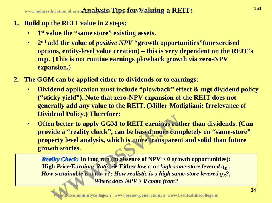
34
Analysis Tips for Valuing a REIT:Analysis Tips for Valuing a REIT:
1.1. Build up the REIT value in 2 steps:Build up the REIT value in 2 steps:•• 11stst value the value the ““same storesame store”” existing assets.existing assets.•• 22ndnd add the value of add the value of positive NPVpositive NPV ““growth growth opportunitiesopportunities””(unexercised(unexercised
options, entityoptions, entity--level value creation) level value creation) –– this is very dependent on the this is very dependent on the REITREIT’’ssmgt. (This is not routine earnings plowback growth via zeromgt. (This is not routine earnings plowback growth via zero--NPV NPV expansion.)expansion.)
2.2. The GGM can be applied either to dividends or to earnings:The GGM can be applied either to dividends or to earnings:•• Dividend application must include Dividend application must include ““plowbackplowback”” effect & mgt dividend policy effect & mgt dividend policy
((““sticky yieldsticky yield””). Note that zero). Note that zero--NPV expansion of the REIT does not NPV expansion of the REIT does not generally add any value to the REIT. (Millergenerally add any value to the REIT. (Miller--Modigliani: Irrelevance of Modigliani: Irrelevance of Dividend Policy.) Therefore:Dividend Policy.) Therefore:
•• Often better to apply GGM to REIT earnings rather than dividendsOften better to apply GGM to REIT earnings rather than dividends. (Can . (Can provide a provide a ““reality checkreality check””, can be based more completely on , can be based more completely on ““samesame--storestore””property level analysis, which is more transparent and solid thaproperty level analysis, which is more transparent and solid than future n future growth stories.growth stories.
Reality Check: Reality Check: In long run (in absence of NPV > 0 growth opportunities):In long run (in absence of NPV > 0 growth opportunities):High High Price/Earnings RatioPrice/Earnings Ratio Either Either low rlow r, or , or high samehigh same--store levered store levered ggEE ..How sustainable is a low r?; How realistic is a high sameHow sustainable is a low r?; How realistic is a high same--store levered store levered ggEE?; ?;
Where does NPV > 0 come from?Where does NPV > 0 come from?
www.bsscommunitycollege.in www.bssnewgeneration.in www.bsslifeskillscollege.in
161www.onlineeducation.bharatsevaksamaj.net www.bssskillmission.in
WWW.BSSVE.IN
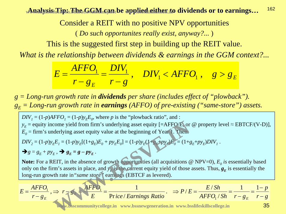
35
Analysis Tip: The GGM can be applied either to dividends or to eAnalysis Tip: The GGM can be applied either to dividends or to earningsarnings……
EE
ggAFFODIVgr
DIVgr
AFFOE ><−
=−
= ,, 1111
DIV1 = (1-p)AFFO1 = (1-p)yEE0, where p is the “plowback ratio”, and :yE = equity income yield from firm’s underlying asset equity [=AFFO/E, or @ property level ≈ EBTCF/(V-D)], E0 = firm’s underlying asset equity value at the beginning of Year 1. Then:
DIV2 = (1-p)yEE1 = (1-p)yE[(1+gE)E0 + pyEE0] = (1-p)yE(1+gE+pyE)E0 = (1+gE+pyE)DIV1 .
g = gE + pyE , ggEE = g = g –– pypyEE .
Note:Note: For a REIT, in the absence of growth opportunities (all acquisiFor a REIT, in the absence of growth opportunities (all acquisitions @ NPV=0), tions @ NPV=0), EE00 isis essentially based essentially based only on the firmonly on the firm’’s assets in place, and s assets in place, and yyEE is the current equity yield of those assets. Thus, is the current equity yield of those assets. Thus, ggEE is essentially the is essentially the longlong--run growth rate run growth rate inin““samesame storestore”” earnings (EBTCF as levered).earnings (EBTCF as levered).
grp
grShAFFOShEEP
RatioEarningsiceEAFFOgr
grAFFOE
EE
E −−
=−
==⇒==−⇒−
=11
///.
/Pr1,
1
11
Consider a REIT with no positive NPV opportunities( Do such opportunites really exist, anyway?... )
This is the suggested first step in building up the REIT value.What is the relationship between dividends & earnings in the GGM context?...
g = Long-run growth rate in dividends per share (includes effect of “plowback”).gE = Long-run growth rate in earnings (AFFO) of pre-existing (“same-store”) assets.
www.bsscommunitycollege.in www.bssnewgeneration.in www.bsslifeskillscollege.in
162www.onlineeducation.bharatsevaksamaj.net www.bssskillmission.in
WWW.BSSVE.IN

36
This is g . . .Percent
199219911990198919881987 1993 1994 1995 1996 1997 1998 1999 2000 2001 2002 2003 2004 20050.00
1.00
2.00
3.00
4.00
5.00
6.00
7.00
8.00
9.00
Dividend per Share Growth(Annual year-over-year growth, 1987-2005)
2.40
7.647.09
5.38
2.62
5.41
7.02
5.98
6.76
4.88
7.39
7.977.65
6.67
3.80
1.85
5.17
5.80
4.95
Figure by MIT OCW.www.bsscommunitycollege.in www.bssnewgeneration.in www.bsslifeskillscollege.in
163www.onlineeducation.bharatsevaksamaj.net www.bssskillmission.in
WWW.BSSVE.IN

37
This is not gE because it’s not “same store”…
Compare to previous slide to see “dividend smoothing”.
Percent
1993 1994 1995 1996 1997 1998 1999 2000 2001 2002 2003 2004 20050
5
-5
10
15
20
11.63 12.1411.04
10.35
12.47
18.63
10.88
8.22
(2.44)
2.523.32
2.33
(3.85)
FFO Per Share Growth(Year-over-year growth, 1993-2005)
Note: Data for 1994-1999 based on partial information for the Top 100 equity REITs
Figure by MIT OCW.
www.bsscommunitycollege.in www.bssnewgeneration.in www.bsslifeskillscollege.in
164www.onlineeducation.bharatsevaksamaj.net www.bssskillmission.in
WWW.BSSVE.IN

38
)(
)()1(
1
1
iesopportunitgrowthNPVgr
AFFO
iesopportunitgrowthNPVgr
AFFOpE
E
+−
=
+−
−=
*)1(
)( 11 grp
shareperAFFOP
AFFOE
−−
==NPV >0 growth NPV >0 growth oppsopps. result in high . result in high REIT price to earnings multiples REIT price to earnings multiples
*)1(
*11
grAFFOp
grDIV
−−
=−
=Collapsing it into the GGM framework: g* is larger than g without growth opportunities.
Value of assets in place less debt
This brings us to third of three steps to deriving This brings us to third of three steps to deriving g*g* in GGM: in GGM: E = DIVE = DIV11 / ( r / ( r –– g* )g* ) ::
1.1. 11stst step was to start with realistic samestep was to start with realistic same--store growth rate: store growth rate: ggEE ..2.2. 22ndnd step was to then consider realistic sustainable step was to then consider realistic sustainable plowback plowback rate ( rate ( pp ) to get: ) to get:
gg = = ggEE + + pypyEE (where (where yyEE = levered equity cash yield of properties: EBTCF / V (less = levered equity cash yield of properties: EBTCF / V (less entity level G&A).entity level G&A).
3.3. Finally now add effect (if any) of positive NPV opportunities (mFinally now add effect (if any) of positive NPV opportunities (micro level options, icro level options, entityentity--level value creation) to get level value creation) to get g*g*, where , where g*g* ≥≥ gg ::
Value of Firm (E) = Value of Existing Assets in Place (less dValue of Firm (E) = Value of Existing Assets in Place (less debt) ebt) + Net Value of Growth Opportunities + Net Value of Growth Opportunities
www.bsscommunitycollege.in www.bssnewgeneration.in www.bsslifeskillscollege.in
165www.onlineeducation.bharatsevaksamaj.net www.bssskillmission.in
WWW.BSSVE.IN

39
Summary & review up to here . . . Summary & review up to here . . .
Same store growth ( Same store growth ( ggEE ) ) (existing property cash flow growth) is pretty (existing property cash flow growth) is pretty mundanemundane::•• Easy to quantify, Easy to predict,Easy to quantify, Easy to predict,•• Usually not very exciting (R.E. Usually not very exciting (R.E. ““bricks & mortarbricks & mortar”” are are ““cash cowscash cows””, not , not ““growth growth starsstars””, though use of , though use of leverageleverage can make more exciting).can make more exciting).
Growth opportunities ( g* )Growth opportunities ( g* ) (NPV>0 actions) is the more interesting source of growth:(NPV>0 actions) is the more interesting source of growth:•• More uncertain & difficult to predict (how realistic?, How sustMore uncertain & difficult to predict (how realistic?, How sustainable?),ainable?),•• More volatility in More volatility in mktmkt expectnsexpectns about magnitude of NPV>0 opportunities.about magnitude of NPV>0 opportunities.
Positive NPV growth opportunities:Positive NPV growth opportunities:Micro (property) level:Micro (property) level: Buy Low or Sell High Deals; Buy Low or Sell High Deals; ““ArbitrageArbitrage”” betwbetw publpubl & & privpriv mktsmkts; ; Entrepreneurial/Innovative Entrepreneurial/Innovative DevlopmentDevlopment; Creative Mgt of Operations.; Creative Mgt of Operations.Macro (firm) level:Macro (firm) level: Economies of Scale; Franchise Value; Rental Economies of Scale; Franchise Value; Rental MktMkt Dominance; etc.Dominance; etc.
g*g* is very important ( 1 pt is very important ( 1 pt ΔΔg* g* >> ≈≈ 20% 20% ΔΔEE )). Reflects:. Reflects:•• LR growth in EBTCF (LR growth in EBTCF (sustainablesustainable ““same store growthsame store growth”” + + ““plowbackplowback””).).•• LR ability of REIT mgt to generate LR ability of REIT mgt to generate ““growth opportunitiesgrowth opportunities”” (NPV>0 (NPV>0 projects): difference between projects): difference between g*g* and and gg (or (or ggEE ).).
Plowback ( g ) Plowback ( g ) (NPV=0 acquisition of assets) is more uncertain:(NPV=0 acquisition of assets) is more uncertain:•• How long can firm find new acquisitions at NPV=0?How long can firm find new acquisitions at NPV=0?•• But analyst can But analyst can ““shortshort--cutcut”” around this question by using AFFO (earnings) around this question by using AFFO (earnings) version of GGM (as noted on previous slides).version of GGM (as noted on previous slides).
www.bsscommunitycollege.in www.bssnewgeneration.in www.bsslifeskillscollege.in
166www.onlineeducation.bharatsevaksamaj.net www.bssskillmission.in
WWW.BSSVE.IN

40The Dividend (Gordon) Growth Model of REIT Share Prices: A Summary
+ NPV(growth opportunities)
Internally Financed Expansion but no GrowthOpportunities
Internally Financed Expansion and GrowthOpportunities
No expansion [no plowback (p = 0), DIV1 = AFFO1]Case 1:
Case 2:
Case 3:
r - gE
r - g
0 < p < 1
g = gE + p(r - gE ) = gE + pyE
AFFO1 NPV(growth opportunities)
r - g r - g r - gE E = DIV1 (1 - p)AFFO1 AFFO1
E = DIV1r - gE r - gE =
= =
AFFO1
+
(1 - p)AFFO1
=
E + NPV(growth opportunities)E* =
E* =
(1 - p)AFFO1r - g*=E* =
DIV1r - g*
Assumptions about growth environment
Figure by MIT OCW, adapted from course textbook.www.bsscommunitycollege.in www.bssnewgeneration.in www.bsslifeskillscollege.in
167www.onlineeducation.bharatsevaksamaj.net www.bssskillmission.in
WWW.BSSVE.IN

41
23.2.3 Fundamental Growth Opportunities23.2.3 Fundamental Growth OpportunitiesAre Are REITsREITs growth stocksgrowth stocks or or income stocksincome stocks??……
millionmillionmillionEBOB 1000$10.0
100$0.010.0
100$==
−=
Beneficial of Boston (Beneficial of Boston (BOBBOB): An ): An ““income REITincome REIT”…”…
Owns properties that pay $100 million / yr, in perpetuity, no deOwns properties that pay $100 million / yr, in perpetuity, no debt.bt.
OCC = OCC = rr = 10%; = 10%; gg = 0.= 0.
Using GGM, Using GGM, BOBBOB’’ss equity is worth:equity is worth:
www.bsscommunitycollege.in www.bssnewgeneration.in www.bsslifeskillscollege.in
168www.onlineeducation.bharatsevaksamaj.net www.bssskillmission.in
WWW.BSSVE.IN

42
Sioux Realty (Sioux Realty (SiouxSioux): A ): A ““growth REITgrowth REIT”…”…
Sioux owns stabilized operating properties like Sioux owns stabilized operating properties like BOBBOB’’ss that pay $50 that pay $50 million / yr in perpetuity, no debt, million / yr in perpetuity, no debt, plus:plus:
Land on which a completed project worth $3000 million in one yeaLand on which a completed project worth $3000 million in one year can r can be built, at a cost of $2400 million construction. Due to the ribe built, at a cost of $2400 million construction. Due to the risk in this sk in this development project (note the operational leverage), the OCC fordevelopment project (note the operational leverage), the OCC for this this project is 20%.project is 20%.
Thus, SiouxThus, Sioux’’s value is:s value is:
millionmillion
millionmillionGrowthPVExistingPVESIOUX
1000$)500$500($
20.01600$
0.010.050$
)()(
=+=
++
−=
+=
www.bsscommunitycollege.in www.bssnewgeneration.in www.bsslifeskillscollege.in
169www.onlineeducation.bharatsevaksamaj.net www.bssskillmission.in
WWW.BSSVE.IN

43
BOBBOB’’ss and Siouxand Sioux’’s Price/Earnings multiples are:s Price/Earnings multiples are:
( ) 10100$1000$/ ==
millionmillionAFFOE BOB
( ) 2050$
1000$/ ==millionmillionAFFOE SIOUX
If they pay out all their income as dividends, what are the currIf they pay out all their income as dividends, what are the current yields of ent yields of these two these two REITsREITs?? Answer: BOB yield = 10%, Sioux yield = 5%.
Why is Sioux a Why is Sioux a ““growth REITgrowth REIT””??……
Is it because Sioux Is it because Sioux ““does development projectsdoes development projects””??……
Suppose Sioux did not already own the land (and were similar to the “second best developer” on the site)?
www.bsscommunitycollege.in www.bssnewgeneration.in www.bsslifeskillscollege.in
170www.onlineeducation.bharatsevaksamaj.net www.bssskillmission.in
WWW.BSSVE.IN

44
Growth stocks have positive NPV opportunities.Growth stocks have positive NPV opportunities.Value of Firm = Value of Existing Assets in Place (less debt) Value of Firm = Value of Existing Assets in Place (less debt) Equity (E)Equity (E) + Net Value of Growth Opportunities + Net Value of Growth Opportunities
)(
)()1(
1
1
iesopportunitgrowthNPVgr
AFFO
iesopportunitgrowthNPVgr
AFFOpE
E
+−
=
+−
−=
*11
)1()( gr
pshareperAFFO
PAFFO
E−−
==
NPV >0 growth NPV >0 growth oppsopps. result in high REIT price to earnings multiples . result in high REIT price to earnings multiples ……
*1
*1 )1(
grAFFOp
grDIV
−−
=−
=Collapsing it into the GGM framework: g* is larger than g without growth opportunities.
Value of assets in place less debt
www.bsscommunitycollege.in www.bssnewgeneration.in www.bsslifeskillscollege.in
171www.onlineeducation.bharatsevaksamaj.net www.bssskillmission.in
WWW.BSSVE.IN

45
23.2.423.2.4““Most Most REITsREITs are not growth stocks most of the time, are not growth stocks most of the time, but some but some REITsREITs are growth stocks most of the time, are growth stocks most of the time, and most and most REITsREITs are growth stocks some of the time.are growth stocks some of the time.””
Last case is possible because ofLast case is possible because of……
Typical sources of growth Typical sources of growth (NPV > 0)(NPV > 0) opportunities in opportunities in REITsREITs (if any):(if any):
• Developable land already owned.• Entrepreneurial abilities (in devlpt, or possibly other activities).• Macro-level abilities
(scale economies?, franchise value?, econ of scope?).
• Differential property asset valuation in stock vs private property markets.
www.bsscommunitycollege.in www.bssnewgeneration.in www.bsslifeskillscollege.in
172www.onlineeducation.bharatsevaksamaj.net www.bssskillmission.in
WWW.BSSVE.IN

46Based on Green Street P/NAV data and NAREIT Equity Price Index.
23.2.5 Parallel Asset Markets and NAV23.2.5 Parallel Asset Markets and NAV--Based ValuationBased Valuation
-40%
-30%
-20%
-10%
0%
10%
20%
30%
40%Ja
n-90
Jan-
91
Jan-
92
Jan-
93
Jan-
94
Jan-
95
Jan-
96
Jan-
97
Jan-
98
Jan-
99
Jan-
00
Jan-
01
Jan-
02
Jan-
03
Jan-
04
Jan-
05
Jan-
06
Source: Green Street Advisors
Avg
Pre
m =
% (S
hare
Pric
e-N
AV)
/NA
VPublicPublic versus PrivatePrivate Market Pricing of Real Estate Equity …REIT Share Price Premium to NAVREIT Share Price Premium to NAV
www.bsscommunitycollege.in www.bssnewgeneration.in www.bsslifeskillscollege.in
173www.onlineeducation.bharatsevaksamaj.net www.bssskillmission.in
WWW.BSSVE.IN
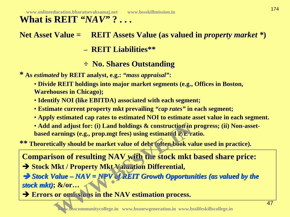
47
What is REIT What is REIT ““NAVNAV”” ? . . .? . . .Net Asset Value = REIT Assets Value (as valued in Net Asset Value = REIT Assets Value (as valued in property market *property market *))
–– REIT Liabilities**REIT Liabilities**
÷÷ No. Shares OutstandingNo. Shares Outstanding** As As estimatedestimated by REIT analyst, e.g.: by REIT analyst, e.g.: ““mass appraisalmass appraisal””::
•• Divide REIT holdings into major market segments (e.g., Offices Divide REIT holdings into major market segments (e.g., Offices in Boston, in Boston, Warehouses in Chicago);Warehouses in Chicago);•• Identify NOI (like EBITDA) associated with each segment;Identify NOI (like EBITDA) associated with each segment;•• Estimate current property Estimate current property mktmkt prevailing prevailing ““cap ratescap rates”” in each segment;in each segment;•• Apply estimated cap rates to estimated NOI to estimate asset vaApply estimated cap rates to estimated NOI to estimate asset value in each segment.lue in each segment.•• Add and adjust for: (i) Land holdings & construction in progresAdd and adjust for: (i) Land holdings & construction in progress; (ii) Nons; (ii) Non--assetasset--based earnings (e.g., based earnings (e.g., prop.mgtprop.mgt fees) using estimated P/E ratio.fees) using estimated P/E ratio.
**** Theoretically should be market value of debt (often book value Theoretically should be market value of debt (often book value used in practice).used in practice).
Comparison of resulting NAV with the stock Comparison of resulting NAV with the stock mktmkt based share price:based share price:Stock Stock MktMkt / Property / Property MktMkt Valuation Differential, Valuation Differential, Stock Value Stock Value –– NAV = NPV of REIT Growth Opportunities (as valued by the NAV = NPV of REIT Growth Opportunities (as valued by the
stock stock mktmkt)); &/or; &/or……Errors or omissions in the NAV estimation process.Errors or omissions in the NAV estimation process.
www.bsscommunitycollege.in www.bssnewgeneration.in www.bsslifeskillscollege.in
174www.onlineeducation.bharatsevaksamaj.net www.bssskillmission.in
WWW.BSSVE.IN

48
Private Property Market
Share Price = (AFFO/share)*(P/AFFO Multiple)Share Price = (NAV/share)*(Prem. to NAV)
Valuation
Effective Gross Income (EGI) - Operating Expenses (OEs) = Net Operating Income (NOI) - Corporate Overhead (G&A Expenses) = EBITDA (Earnings Before Interest, Taxes, Depreciation, and Amortization) - Interest = Funds from Operations (FFO) - Adjustment for Straight-Lining Rents - Amortization of Mortgage Debt - Capital Improvement Expenditures (CI) = Adjusted Funds from Operations (AFFO)
Annual Cash Flows from Operations
Public REIT Market
Annual Cash Flows from Operations
Effective Gross Income (EGI) - Operating Expenses (OEs) = Net Operating Income (NOI) - Capital Improvement Expenditures (CI) = Property-Before-Tax Cash Flow (PBTCF) - Debt Service (DS) = Equity-Before-Tax Cash Flow (EBTCF)
Valuation
Asset Value = NOI
Cap Rate
Cash Flows and Asset Valuation in the Private Property and Public REIT Markets
Figure by MIT OCW, adapted from course textbook.
www.bsscommunitycollege.in www.bssnewgeneration.in www.bsslifeskillscollege.in
175www.onlineeducation.bharatsevaksamaj.net www.bssskillmission.in
WWW.BSSVE.IN

49
Another perspective on this same point (from Chapter 12) Another perspective on this same point (from Chapter 12) ……
0.6
0.8
1.0
1.2
1.4
1.6
1.8
2.0
2.2
2.4
2.6Ja
n-90
Jul-9
0
Jan-
91Ju
l-91
Jan-
92
Jul-9
2
Jan-
93Ju
l-93
Jan-
94Ju
l-94
Jan-
95Ju
l-95
Jan-
96
Jul-9
6
Jan-
97Ju
l-97
Jan-
98Ju
l-98
Jan-
99Ju
l-99
Jan-
00
Jul-0
0
Jan-
01Ju
l-01
Jan-
02Ju
l-02
Jan-
03Ju
l-03
Jan-
04
Jul-0
4
Jan-
05Ju
l-05
Jan-
06
NA
REI
T an
d N
AV
Indi
ces
(NA
REI
T=1
Jan
1990
)
NAREIT Share Price Green Street NAV Ratio (Price/NAV)
www.bsscommunitycollege.in www.bssnewgeneration.in www.bsslifeskillscollege.in
176www.onlineeducation.bharatsevaksamaj.net www.bssskillmission.in
WWW.BSSVE.IN

50
Exhibit 7-4:End of Year Public vs Private Asset Mkt Commercial R.E. Values:
(Indexes set to have Equal Avg Values 1974-2006)
0.6
1.1
1.6
2.1
2.6
3.1
3.6
4.1
74 76 78 80 82 84 86 88 90 92 94 96 98 00 02 04 06
NAREIT (Unlevered) NCREIF (Unsmoothed)
Another perspective on this point (update of Exh.7-4 from Chapter 7) . . .
www.bsscommunitycollege.in www.bssnewgeneration.in www.bsslifeskillscollege.in
177www.onlineeducation.bharatsevaksamaj.net www.bssskillmission.in
WWW.BSSVE.IN

51
Another perspective on this point (here monthly, with private R.E. represented by transactions-based indexes) . . .
Indexes of Commercial Property Values: Private vs REITs (2002 = 1.00)
0
0.2
0.4
0.6
0.8
1
1.2
1.4
1.6
1.819
74
1976
1978
1980
1982
1984
1986
1988
1990
1992
1994
1996
1998
2000
2002
2004
2006
PrivateREITs
www.bsscommunitycollege.in www.bssnewgeneration.in www.bsslifeskillscollege.in
178www.onlineeducation.bharatsevaksamaj.net www.bssskillmission.in
WWW.BSSVE.IN

52
Indexes of Commercial Property Values: Private vs REITs (2002 = 1.00)
0.5
0.6
0.7
0.8
0.9
1
1.1
1.2
1.3
1.4
1.5
1.6
1.719
91
1992
1993
1994
1995
1996
1997
1998
1999
2000
2001
2002
2003
2004
2005
2006
PrivateREITs
Zeroing in on 1991-2006 period . . .
www.bsscommunitycollege.in www.bssnewgeneration.in www.bsslifeskillscollege.in
179www.onlineeducation.bharatsevaksamaj.net www.bssskillmission.in
WWW.BSSVE.IN

53
The point is . . .The point is . . .•• REITREIT--based valuations & private property based valuations & private property mktmkt--based valuations appear based valuations appear to be different much of the time.to be different much of the time.
•• These differences do not appear to be explainable by differenceThese differences do not appear to be explainable by differences in the s in the underlying operating cash flows of the underlying operating cash flows of the REITsREITs vsvs the private properties; the private properties; nor are they explainable entirely by purely nor are they explainable entirely by purely firmfirm--levellevel considerations (e.g., considerations (e.g., debt financing, entitydebt financing, entity--level mgt, trading, etc.). level mgt, trading, etc.).
•• Thus, at least part of these differences appear to be Thus, at least part of these differences appear to be micromicro--levellevel valuation valuation differencesdifferences, differences in the two markets, differences in the two markets’’ perceptions of the values of the perceptions of the values of the samesame underlying properties as of the same point in time underlying properties as of the same point in time ((““micromicro--levellevel”” = = ““bricks & mortarbricks & mortar””, underlying assets as opposed to firm, underlying assets as opposed to firm--level effects).level effects).
•• There is some evidence that REIT valuations tend to be a bit moThere is some evidence that REIT valuations tend to be a bit more re volatile, and to volatile, and to leadlead the private property market valuations in time (based the private property market valuations in time (based on timing of major cyclical turning points, the lead may be up ton timing of major cyclical turning points, the lead may be up to 3 years.)o 3 years.)
•• There is also some tentative evidence that the differences betwThere is also some tentative evidence that the differences between the een the two markets may be diminishing in recent years (faster two markets may be diminishing in recent years (faster ““mean reversionmean reversion””of P/NAV differential).of P/NAV differential).
www.bsscommunitycollege.in www.bssnewgeneration.in www.bsslifeskillscollege.in
180www.onlineeducation.bharatsevaksamaj.net www.bssskillmission.in
WWW.BSSVE.IN

54
Major investment issues of the valuation difference:Major investment issues of the valuation difference:1.1. Which market should the investor use to make real estate Which market should the investor use to make real estate
investments: public (REIT), or private (direct property)?investments: public (REIT), or private (direct property)?
2.2. Is there scope for Is there scope for ““arbitragearbitrage”” between the two markets? between the two markets? That is, can (nearly) That is, can (nearly) risklessriskless profits be earned by moving profits be earned by moving assets from one ownership form to the other:assets from one ownership form to the other:•• Taking private assets public via REIT acquisition or IPO?; Taking private assets public via REIT acquisition or IPO?; •• Taking REIT assets private via buyout/privatization or simply viTaking REIT assets private via buyout/privatization or simply via a
sale of assets or secured debt in the private market?sale of assets or secured debt in the private market?
3.3. What is the nature and magnitude of the What is the nature and magnitude of the micromicro--levelleveldifferential valuation (and which value is differential valuation (and which value is ““correctcorrect””)?)?
www.bsscommunitycollege.in www.bssnewgeneration.in www.bsslifeskillscollege.in
181www.onlineeducation.bharatsevaksamaj.net www.bssskillmission.in
WWW.BSSVE.IN

55
Two ways to consider the microTwo ways to consider the micro--level differential valuation:level differential valuation:Longitudinal & CrossLongitudinal & Cross--sectionalsectional
Longitudinal (across time) difference:• REIT mkt leads private market (not perfectly, but…):
• Info flows from Public Private (mkt as whole)(Public mkt more informationally “efficient”.)
Cross-sectional (across REITs) difference:• Private Mkt NAVs contain information (again, not perfect, but…)
• Low P/NAV REITs tend to rise, & vice versa.(Public mkt tends to “overshoot” or “herd”.)• Info can flow from Private Public (specific REITs)
www.bsscommunitycollege.in www.bssnewgeneration.in www.bsslifeskillscollege.in
182www.onlineeducation.bharatsevaksamaj.net www.bssskillmission.in
WWW.BSSVE.IN
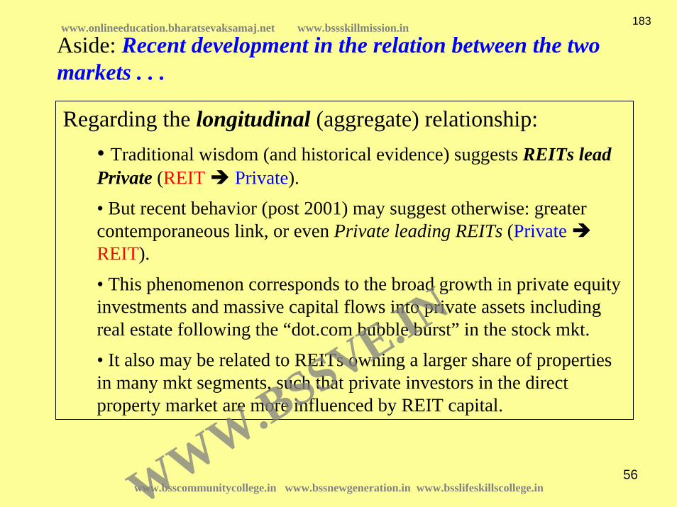
56
Aside: Recent development in the relation between the two markets . . .
Regarding the longitudinal (aggregate) relationship:• Traditional wisdom (and historical evidence) suggests REITs lead Private (REIT Private).• But recent behavior (post 2001) may suggest otherwise: greater contemporaneous link, or even Private leading REITs (PrivateREIT).• This phenomenon corresponds to the broad growth in private equity investments and massive capital flows into private assets including real estate following the “dot.com bubble burst” in the stock mkt.• It also may be related to REITs owning a larger share of properties in many mkt segments, such that private investors in the direct property market are more influenced by REIT capital.
www.bsscommunitycollege.in www.bssnewgeneration.in www.bsslifeskillscollege.in
183www.onlineeducation.bharatsevaksamaj.net www.bssskillmission.in
WWW.BSSVE.IN

57
Time
Mkt
Inde
x Va
lue
Leve
ls
Private
Public
If Public Private, then: • Public > Private when values are rising; • Private > Public when values are falling.
www.bsscommunitycollege.in www.bssnewgeneration.in www.bsslifeskillscollege.in
184www.onlineeducation.bharatsevaksamaj.net www.bssskillmission.in
WWW.BSSVE.IN

58
Time
Mkt
Inde
x Va
lue
Leve
ls
Private
Public
If Private Public, then: • Private > Public when values are rising; • Public > Private when values are falling.
www.bsscommunitycollege.in www.bssnewgeneration.in www.bsslifeskillscollege.in
185www.onlineeducation.bharatsevaksamaj.net www.bssskillmission.in
WWW.BSSVE.IN

59
Exhibit 7-4:End of Year Public vs Private Asset Mkt Commercial R.E. Values:
(Indexes set to have Equal Avg Values 1974-2006)
0.6
1.1
1.6
2.1
2.6
3.1
3.6
4.1
74 76 78 80 82 84 86 88 90 92 94 96 98 00 02 04 06
NAREIT (Unlevered) NCREIF (Unsmoothed)
Red used to be left of blue, but lately the opposite . . .
www.bsscommunitycollege.in www.bssnewgeneration.in www.bsslifeskillscollege.in
186www.onlineeducation.bharatsevaksamaj.net www.bssskillmission.in
WWW.BSSVE.IN

60
Indexes of Commercial Property Values: Private vs REITs (2002 = 1.00)
0.5
0.6
0.7
0.8
0.9
1
1.1
1.2
1.3
1.4
1.5
1.6
1.719
91
1992
1993
1994
1995
1996
1997
1998
1999
2000
2001
2002
2003
2004
2005
2006
PrivateREITs
Red used to be left of blue, but lately the opposite . . .
Recently (since 2004), private mktvaluations seem to be above public mkt valuations when mkt is rising.
Private mkt leading public?
(Price discovery in private mkt?)
Will this shift in locus of price discovery remain?...
www.bsscommunitycollege.in www.bssnewgeneration.in www.bsslifeskillscollege.in
187www.onlineeducation.bharatsevaksamaj.net www.bssskillmission.in
WWW.BSSVE.IN
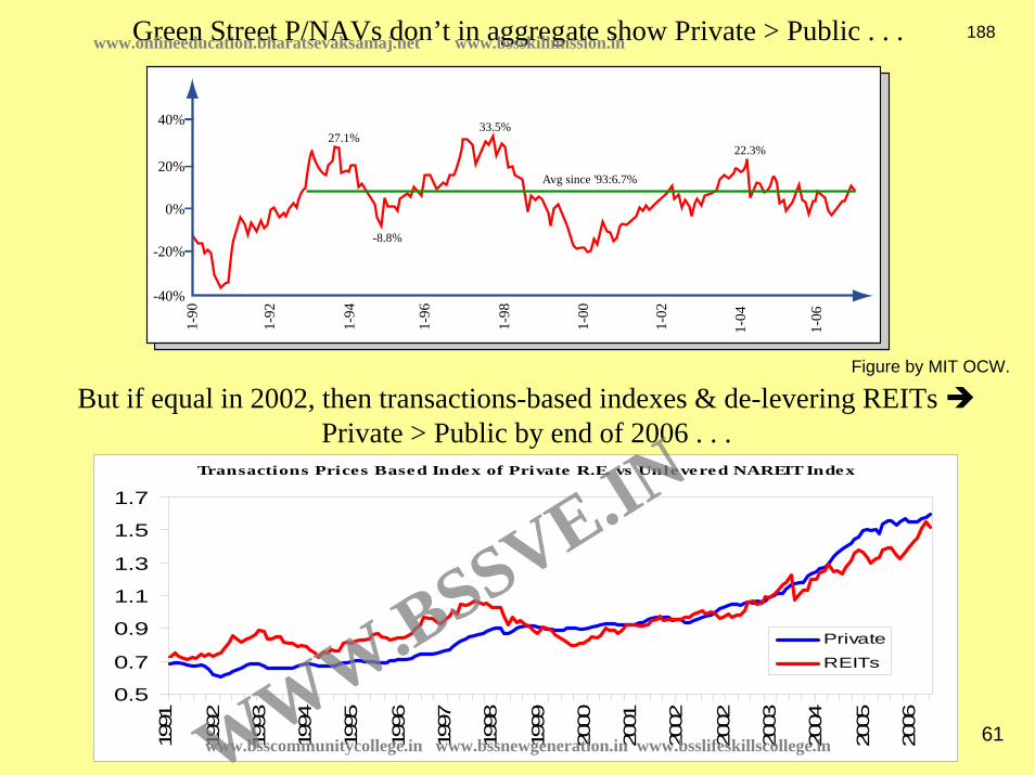
61
Green Street P/NAVs don’t in aggregate show Private > Public . . .
But if equal in 2002, then transactions-based indexes & de-levering REITsPrivate > Public by end of 2006 . . .
Transactions Prices Based Index of Private R.E. vs Unlevered NAREIT Index
0.5
0.7
0.9
1.1
1.3
1.5
1.7
1991
1992
1993
1994
1995
1996
1997
1998
1999
2000
2001
2002
2002
2003
2004
2005
2006
Private
REITs
-40%
-20%
0%
20%
40%
1-90
1-92
1-94
1-96
1-98
1-00
1-02
1-04
1-06
27.1%33.5%
22.3%
-8.8%
Avg since '93:6.7%
Figure by MIT OCW.
www.bsscommunitycollege.in www.bssnewgeneration.in www.bsslifeskillscollege.in
188www.onlineeducation.bharatsevaksamaj.net www.bssskillmission.in
WWW.BSSVE.IN

62
Definition of the microDefinition of the micro--level valuation difference:level valuation difference:For specific individual properties:For specific individual properties:
IVIVREITREIT ≠≠ MVMVPRIVPRIV
(Recall that stock mkt makes: IVREIT=MVREIT in share price.
Thus, if a microThus, if a micro--level valuation difference exists, then profitable (NPV > 0) level valuation difference exists, then profitable (NPV > 0) opportunities exist for opportunities exist for REITsREITs by buying or selling properties in the private by buying or selling properties in the private property market.property market.
This is often referred to as (positive or negative) This is often referred to as (positive or negative) ““accretionaccretion”” opportunity for opportunity for REITsREITs::
REIT Buying: REIT Buying: NPVNPVMVMV(REIT) = NPV(REIT) = NPVIVIV(REIT) = IV(REIT) = IVREITREIT –– MVMVPRIVPRIV
REIT Selling: REIT Selling: NPVNPVMVMV(REIT) = NPV(REIT) = NPVIVIV(REIT) = MV(REIT) = MVPRIVPRIV –– IVIVREITREIT
Mitigated by transaction costs and management or firmMitigated by transaction costs and management or firm--level considerations.level considerations.
From Chapter 12 (Section 12.3)From Chapter 12 (Section 12.3)……
www.bsscommunitycollege.in www.bssnewgeneration.in www.bsslifeskillscollege.in
189www.onlineeducation.bharatsevaksamaj.net www.bssskillmission.in
WWW.BSSVE.IN

63
When REIT valuation > Private valuation (positive REIT premium tWhen REIT valuation > Private valuation (positive REIT premium to o NAV):NAV):•• REITsREITs have growth opportunities (NPV>0, have growth opportunities (NPV>0, ““accretionaccretion””) from ) from buyingbuying in the in the private market.private market.•• REITsREITs raise capital by issuing stock in the public raise capital by issuing stock in the public mktmkt, use proceeds to buy , use proceeds to buy properties.properties.
When REIT valuation < Private valuation (negative REIT premium tWhen REIT valuation < Private valuation (negative REIT premium to o NAV):NAV):•• REITsREITs are no longer are no longer ““growth stocksgrowth stocks””, and their shares are re, and their shares are re--priced accordingly priced accordingly in the stock market (price/earnings multiples fall, in the stock market (price/earnings multiples fall, REITsREITs are priced like are priced like ““value value stocksstocks””, or , or ““income stocksincome stocks””).).•• In the extreme, In the extreme, REITsREITs may become may become ““shrinking stocksshrinking stocks””, maximizing shareholder , maximizing shareholder value by selling off property equity (or debt) and paying out prvalue by selling off property equity (or debt) and paying out proceeds in dividends.oceeds in dividends.
The 2 The 2 mktsmkts swing between these 2 conditions, also with periods when they swing between these 2 conditions, also with periods when they are nearly equal valued.are nearly equal valued.Little Little ““arbitrage tradingarbitrage trading”” occurs when the 2 occurs when the 2 mktsmkts are within 5%are within 5%--10% of 10% of each othereach other’’s valuations (due to transaction costs, firms valuations (due to transaction costs, firm--level effects).level effects).Arbitrage trading tends to keep valuation differences to less tArbitrage trading tends to keep valuation differences to less than 15%han 15%--20%, but occasionally greater differences have briefly occurred.20%, but occasionally greater differences have briefly occurred.
www.bsscommunitycollege.in www.bssnewgeneration.in www.bsslifeskillscollege.in
190www.onlineeducation.bharatsevaksamaj.net www.bssskillmission.in
WWW.BSSVE.IN

64
How can a REIT How can a REIT ““remain a public REIT in businessremain a public REIT in business””, and still maximize , and still maximize shareholder value during times when the stock market valuation oshareholder value during times when the stock market valuation of real estate is f real estate is less thanless than the private property market valuation? . . .the private property market valuation? . . .
IVIVREITREIT < MV< MVPRIVPRIV
•• Sell into the private market most but not all of the equity in Sell into the private market most but not all of the equity in many of their properties (e.g., many of their properties (e.g., sell properties into a partnership controlled by the REIT, with sell properties into a partnership controlled by the REIT, with passive equity partners), passive equity partners), paying out proceeds in extraordinary dividends (or stock purchaspaying out proceeds in extraordinary dividends (or stock purchases), while retaining es), while retaining effective operational control over the assets (e.g., sell to effective operational control over the assets (e.g., sell to passivepassive partners, such as pension partners, such as pension funds): funds): REIT retains scale & operational product.REIT retains scale & operational product.
•• Issue secured debt (mortgages) collateralized by the excess of Issue secured debt (mortgages) collateralized by the excess of MVMVPRIVPRIV over IVover IVREITREIT , paying , paying out proceeds as extraordinary dividends. out proceeds as extraordinary dividends. (( Risky.)Risky.)
•• Sell some of their properties outright into the private market Sell some of their properties outright into the private market (paying proceeds as dividends (paying proceeds as dividends or stock purchase), but subject to contracts to retain the REIT or stock purchase), but subject to contracts to retain the REIT as property manager (TRS).as property manager (TRS).
•• If private market valuations are sufficiently high (and expecteIf private market valuations are sufficiently high (and expected to remain so), consider d to remain so), consider going into development projects with most financing coming from going into development projects with most financing coming from external private equity external private equity and debt sources: and debt sources: Use the Use the REITREIT’’ss entrepreneurial capability; Use developable land entrepreneurial capability; Use developable land already owned; Maximize leverage of private market valuationalready owned; Maximize leverage of private market valuation. . (Note: Though tempting, this (Note: Though tempting, this strategy is risky at the peak of a private market cycle.)strategy is risky at the peak of a private market cycle.)
•• Reinvest proceeds from domestic private market sales into interReinvest proceeds from domestic private market sales into international real estate assets national real estate assets where valuations are lower (yields are higher).where valuations are lower (yields are higher).
www.bsscommunitycollege.in www.bssnewgeneration.in www.bsslifeskillscollege.in
191www.onlineeducation.bharatsevaksamaj.net www.bssskillmission.in
WWW.BSSVE.IN

65
The OCCThe OCC--based source: Marketbased source: Market--wide valuation differences:wide valuation differences:•• Affects all properties, all Affects all properties, all REITsREITs..•• Reflects different informational efficiency (REIT lead).Reflects different informational efficiency (REIT lead).•• Reflects different investor clienteles and different market funReflects different investor clienteles and different market functioning ctioning leading to different liquidity, different risk & return patternsleading to different liquidity, different risk & return patterns in the in the investment results, causing differential perceptions or pricing investment results, causing differential perceptions or pricing of risk.of risk.
Causes of microCauses of micro--level valuation differential:level valuation differential:
The CFThe CF--based source: Idiosyncratic valuation differences:based source: Idiosyncratic valuation differences:•• Affects specific properties or specific Affects specific properties or specific REITsREITs..•• Caused by differential ability to generate firmCaused by differential ability to generate firm--level incremental CF level incremental CF from same properties (e.g., REIT scale economies, franchise valufrom same properties (e.g., REIT scale economies, franchise value, space e, space market monopoly power, adjacent prop spillover, etc.)market monopoly power, adjacent prop spillover, etc.)
Two possible sources: Two possible sources: CFsCFs & OCC& OCC(Recall DCF valuation formula.)
Note: Some REIT mgt actions, such as capital structure (financinNote: Some REIT mgt actions, such as capital structure (financing of the g of the REIT), property REIT), property devlptdevlpt or trading strategy, etc., affect firmor trading strategy, etc., affect firm--level REIT value level REIT value but not microbut not micro--level property valuation (of existing assets in place).level property valuation (of existing assets in place).
www.bsscommunitycollege.in www.bssnewgeneration.in www.bsslifeskillscollege.in
192www.onlineeducation.bharatsevaksamaj.net www.bssskillmission.in
WWW.BSSVE.IN

66
Which valuation is Which valuation is ““correctcorrect””? . . .? . . .Would you believeWould you believe……
They both are?They both are?(Each in their own way, for their relevant investor clientele.)(Each in their own way, for their relevant investor clientele.)
But keep in mindBut keep in mind……
•• Tendency of REIT market to Tendency of REIT market to leadlead private private mktmkt (sometimes (sometimes up to 3 years). up to 3 years). (Recall longitudinal difference noted earlier.)(Recall longitudinal difference noted earlier.)
•• Tendency of REIT market to exhibit Tendency of REIT market to exhibit ““excess volatilityexcess volatility””::•• transient transient ““overshootingovershooting”” of valuation changes, followed by of valuation changes, followed by ““correctionscorrections””. (Also recall cross. (Also recall cross--sectional difference noted earlier.)sectional difference noted earlier.)
•• Two markets sometimes exhibit a Two markets sometimes exhibit a ““tortoise & haretortoise & hare””relationship (both can relationship (both can ““learnlearn”” from the other).from the other).
www.bsscommunitycollege.in www.bssnewgeneration.in www.bsslifeskillscollege.in
193www.onlineeducation.bharatsevaksamaj.net www.bssskillmission.in
WWW.BSSVE.IN

67
12.3.5:12.3.5: Risk is in the Risk is in the objectobject not in the not in the beholderbeholder..
(Remember from Ch.10: Match (Remember from Ch.10: Match disc.ratedisc.rate to the risk of the to the risk of the investment whose investment whose CFsCFs are being discounted.)are being discounted.)
Property "X" has the same risk for Investor "A" as for Investor "B".
Therefore, oppty cost of cap (r) is same for “A” & “B” for purposes of evaluating NPV of investment in “X” (same discount rate).
Unless, say, “A” has some unique ability to alter the risk of X’s future CFs. (This is rare: be skeptical of such claims!)
It is worth reviewing Section 12.3.5 at this pointIt is worth reviewing Section 12.3.5 at this point……
www.bsscommunitycollege.in www.bssnewgeneration.in www.bsslifeskillscollege.in
194www.onlineeducation.bharatsevaksamaj.net www.bssskillmission.in
WWW.BSSVE.IN

68
Example...
REIT A has expected total return to equity = 12%, Avg.debt int.rate = 7%, Debt/Total Asset Value Ratio = 20%
What is REIT A’s (firm-level) Cost of Capital (WACC)?
Ans: (0.2)7% + (1-0.2)12% = 1.4% + 9.6% = 11%.
REIT B has no debt, curr.div.yield = 6%, pays out all its earnings in dividends (share price/earnings multiple = 16.667), avg.div. growth rate = 4%/yr.
What is REIT B’s (firm-level) Cost of Capital (WACC)?[Hint: Use “Gordon Growth Model”: r = y + g.]
Ans: 6% + 4% = 10%.
www.bsscommunitycollege.in www.bssnewgeneration.in www.bsslifeskillscollege.in
195www.onlineeducation.bharatsevaksamaj.net www.bssskillmission.in
WWW.BSSVE.IN

69
Example (cont.)...Property X is a Boston Office Bldg, in a market where such bldgs sell at 8% cap
rates (CF / V), with 0.5% expected LR annual growth (in V & CF). It has initial CF = $1,000,000/yr.
How much can REIT A afford to pay for How much can REIT A afford to pay for Prop.XProp.X, without suffering loss , without suffering loss in share value, if the REIT market currently has a 10% premium oin share value, if the REIT market currently has a 10% premium over ver the private property market in valuation?the private property market in valuation?
Answer: $13,750,000, analyzed as follows…Prop.X Val in Priv.Mkt = $12,500,000 = $1,000,000 / 0.08= $1,000,000 / (8.5% - 0.5%), where y = r – g, as const.growth perpetuity.Prop.X Val in REIT Mkt = $12,500,000 * 1.1 = $13,750,000, due to 10% premium.Note: “cap rate” in REIT Mkt = 1/13.75 = 7.27%,
OCC for REIT is rX = 7.27% + 0.5% = 7.77%, i.e.: $13.75 = $1/(.0777-.05).Note: • Prop.X value for REIT is not equal to: $1,000,000 / (11% - 0.5%) = $9,524,000.• OCC relevant for valuing Prop.X purchase for REIT is not 11% (REIT A’s firm
level WACC).• Nor is relevant OCC equal to: Prop.X OCC in Private Mkt = 8% + 0.5% = 8.5%.
www.bsscommunitycollege.in www.bssnewgeneration.in www.bsslifeskillscollege.in
196www.onlineeducation.bharatsevaksamaj.net www.bssskillmission.in
WWW.BSSVE.IN

70
Answer: Same as value for REIT A: Prop.X Val for REIT B = $1,000,000 / (7.77% - 0.5%) = $13,750,000.• This is not equal to $1,000,000 / (10%-4%) = $1,000,000 / 6% =
$16,667,000, REIT B’s P/E multiple applied to Prop.X earnings.• Most of REIT B’s assets must be higher risk and higher growth than Prop.X
(perhaps REIT B mostly does development projects).
Same question for REIT B . . .
Example (cont.)...
How much can Private Consortium “C” afford to pay for Prop.X?
Answer: $12,500,000 = $1,000,000 / 0.08 = The Private Mkt’s Value.
How much How much shouldshould either REIT (A or B) pay for either REIT (A or B) pay for Prop.XProp.X??
Answer: $12,500,000, since that is the private mkt MV, unless they have to compete with each other (or other REITs), & the resulting bidding war bids the price up above that.
www.bsscommunitycollege.in www.bssnewgeneration.in www.bsslifeskillscollege.in
197www.onlineeducation.bharatsevaksamaj.net www.bssskillmission.in
WWW.BSSVE.IN

71
Suppose REIT B can borrow money at 6% while REIT A must pay 7% for corporate debt. Does this mean REIT B can afford to pay more for Prop.X than REIT A, assuming both REITs would finance the purchase with corporate-level debt?...
Example (1 last question...)
Answer: No.
• The value of the asset in the firm’s equity is unaffected by it’s corporate cost of debt.
• The firm’s borrowing rate does not generally equal either its firm-level WACC or the specific OCC relevant for a given investment.
www.bsscommunitycollege.in www.bssnewgeneration.in www.bsslifeskillscollege.in
198www.onlineeducation.bharatsevaksamaj.net www.bssskillmission.in
WWW.BSSVE.IN

72
23.2.6 Agency Costs: Conflicts of Interest23.2.6 Agency Costs: Conflicts of Interest
Some major issues to watch out forSome major issues to watch out for……
1) Transaction bias in 1) Transaction bias in UPREITsUPREITs::••Due to taxDue to tax--based conflict (different cost basis for LP investors based conflict (different cost basis for LP investors vsvs public stock public stock investors)?investors)?……
2) Real estate interests outside the REIT:2) Real estate interests outside the REIT:••Do REIT managers have other real estate interests that compete wDo REIT managers have other real estate interests that compete with the ith the REITREIT’’ss properties or for the managersproperties or for the managers’’ time & energy (other properties not in time & energy (other properties not in the REIT, other interests such as brokerage or management firms)the REIT, other interests such as brokerage or management firms)??……
3) Potential for 3) Potential for ““selfself--dealingdealing””::••Do REIT managers have incentives to have the REIT engage in Do REIT managers have incentives to have the REIT engage in ““SweatheartSweatheart””deals with brokerage, management, development firms in which thedeals with brokerage, management, development firms in which they have y have interests?interests?……
4) Take4) Take--over difficulties re over difficulties re ““55--oror--Fewer RuleFewer Rule””::•• REIT governance often makes hostile takeovers particularly diffREIT governance often makes hostile takeovers particularly difficult, in part icult, in part due to due to 55--oror--Fewer Fewer Rule.Rule.
www.bsscommunitycollege.in www.bssnewgeneration.in www.bsslifeskillscollege.in
199www.onlineeducation.bharatsevaksamaj.net www.bssskillmission.in
WWW.BSSVE.IN

73
Public Investors(Stockholders)
Private Investors(Partnership Unit-holders)
REIT
Umbrella Partnership(“Operating Partnership”: OP)
PropertyPartnership
PropertyPartnership
PropertyPartnership
Property Property Property
TheThe
““UPREITUPREIT””
StructureStructure
www.bsscommunitycollege.in www.bssnewgeneration.in www.bsslifeskillscollege.in
200www.onlineeducation.bharatsevaksamaj.net www.bssskillmission.in
WWW.BSSVE.IN

74
23.3 Some Considerations of REIT Management Strategy 23.3 Some Considerations of REIT Management Strategy The traditional real estate cliché about the “3 determinants of value”:
“Location, location, location”.
The modern REIT cliché about the “3 determinants of value”:“Management, management, management”.
Six major strategies or strategic considerationsSix major strategies or strategic considerations……
1) Financial strategy: 1) Financial strategy: ““Caught between a rock and a hard placeCaught between a rock and a hard place”…”…-- REITsREITs dondon’’t have traditional Ct have traditional C--corpcorp income taxincome tax--based rationale for based rationale for
use of debt financing. But use of debt financing. But REITsREITs often need external capital (R.E. is often need external capital (R.E. is capitalcapital--intensive, and intensive, and REITsREITs must pay out 90% of earnings). Various must pay out 90% of earnings). Various considerations enter the REIT capital structure equation:considerations enter the REIT capital structure equation:
•• Stock market wants growth;Stock market wants growth;•• Real estate is not a growth asset without lots of leverage (maReal estate is not a growth asset without lots of leverage (maximized by ximized by shortshort--term or floatingterm or floating--rate debt);rate debt);•• Stock market doesnStock market doesn’’t like t like REITsREITs to be highly levered (especially with to be highly levered (especially with shortshort--term or floatingterm or floating--rate debt).rate debt).
Solution: Solution: walk the tightrope carefullywalk the tightrope carefully..
www.bsscommunitycollege.in www.bssnewgeneration.in www.bsslifeskillscollege.in
201www.onlineeducation.bharatsevaksamaj.net www.bssskillmission.in
WWW.BSSVE.IN

75
23.3 Some REIT Strategic Management Considerations (cont.) 23.3 Some REIT Strategic Management Considerations (cont.)
2) Specialize (2) Specialize (know your marketknow your market):):•• Be a Be a ““residential REITresidential REIT”” or a or a ““retail REITretail REIT””, etc, etc……•• Sometimes some combinations are Sometimes some combinations are ““OKOK”” (e.g., office & industrial)(e.g., office & industrial)•• Geographical specialization is Geographical specialization is ““less coolless cool”” (you (you gottagotta get scale economies get scale economies somehow!)somehow!)
3) Build 3) Build ““franchise valuefranchise value”” ((brand name recognition?brand name recognition?):):••Improve tenant service with increased geographical and product sImprove tenant service with increased geographical and product scope.cope.
4) Consider 4) Consider ““vertical integrationvertical integration””::••Land, Land, DevlptDevlpt, Asset ownership, Property Mgt, Leasing, Tenant , Asset ownership, Property Mgt, Leasing, Tenant SvcsSvcs(logistics, communications, etc), Information (databank);(logistics, communications, etc), Information (databank);••Allows REIT to ride through periods when stock market undervalueAllows REIT to ride through periods when stock market undervalues real s real estate assets relative to the property market (sell most asset oestate assets relative to the property market (sell most asset ownership into wnership into property market, retain control and ancillary functions, possiblproperty market, retain control and ancillary functions, possibly develop y develop new buildings);new buildings);••During periods of low property market asset valuation relative tDuring periods of low property market asset valuation relative to the stock o the stock market, buy existing properties and bank market, buy existing properties and bank buildablebuildable land).land).
www.bsscommunitycollege.in www.bssnewgeneration.in www.bsslifeskillscollege.in
202www.onlineeducation.bharatsevaksamaj.net www.bssskillmission.in
WWW.BSSVE.IN

76
23.3 Some REIT Strategic Management Considerations (cont.) 23.3 Some REIT Strategic Management Considerations (cont.)
5) Take advantage of 5) Take advantage of Economies of Scale Economies of Scale (such as they are):(such as they are):•• Are there scale economies in REIT administrative costs?Are there scale economies in REIT administrative costs?……
•• Are there scale economies in REIT capital costs?Are there scale economies in REIT capital costs?……
•• Where are the limits of such economies?Where are the limits of such economies?……
•• Are there economies of scope in REIT service provision?Are there economies of scope in REIT service provision?……
6) Try to develop some 6) Try to develop some market powermarket power ((““monopoly controlmonopoly control””) in local space ) in local space markets:markets:
•• Buy (or build) most of the space of a given type in a given loBuy (or build) most of the space of a given type in a given local cal submarket;submarket;•• But beware, rare is the submarket that has no potential close But beware, rare is the submarket that has no potential close substitute substitute in the same metro area.in the same metro area.
www.bsscommunitycollege.in www.bssnewgeneration.in www.bsslifeskillscollege.in
203www.onlineeducation.bharatsevaksamaj.net www.bssskillmission.in
WWW.BSSVE.IN

77
REIT scale & consolidation
9
0.13
34
3.07
24
6.29
21 21.38 2023.85
7
18.48
6
26.79
45
40
35
30
25
20
15
10
5
0
Under
$100
M$1
00-$4
99M
$500
-$999
M$1
-$2.49
B$2
.5-$4
.99B
$5-$9
.99B
Over $
10B
# of
REI
Ts a
nd %
of R
EIT
Mar
ket C
apita
lizat
ion
Distribution of Equity REITs by Firm Size (Market Capitalization)
Number of REITs % of REIT Mkt. Cap.
Calculations based on data available at http://www.nareit.org.
Figure by MIT OCW, adapted from course textbook.
www.bsscommunitycollege.in www.bssnewgeneration.in www.bsslifeskillscollege.in
204www.onlineeducation.bharatsevaksamaj.net www.bssskillmission.in
WWW.BSSVE.IN
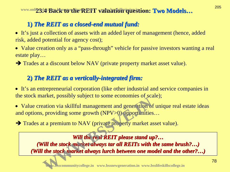
78
23.4 Back to the REIT valuation question: 23.4 Back to the REIT valuation question: Two ModelsTwo Models……
1) 1) The REIT as a closedThe REIT as a closed--end mutual fund:end mutual fund:•• ItIt’’s just a collection of assets with an added layer of management s just a collection of assets with an added layer of management (hence, added (hence, added risk, added potential for agency cost);risk, added potential for agency cost);•• Value creation only as a Value creation only as a ““passpass--throughthrough”” vehicle for passive investors wanting a real vehicle for passive investors wanting a real estate playestate play……
Trades at a discount below NAV (private property market asset vTrades at a discount below NAV (private property market asset value).alue).
2) 2) The REIT as a verticallyThe REIT as a vertically--integrated firm:integrated firm:
•• ItIt’’s an entrepreneurial corporation (like other industrial and servs an entrepreneurial corporation (like other industrial and service companies in ice companies in the stock market, possibly subject to some economies of scale);the stock market, possibly subject to some economies of scale);
•• Value creation via skillful management and generation of uniquValue creation via skillful management and generation of unique real estate ideas e real estate ideas and options, providing some growth (NPV>0) opportunitiesand options, providing some growth (NPV>0) opportunities……
Trades at a premium to NAV (private property market asset valueTrades at a premium to NAV (private property market asset value).).
Will the real REIT please stand up?Will the real REIT please stand up?……(Will the stock market always tar all (Will the stock market always tar all REITsREITs with the same brush?with the same brush?……))
(Will the stock market always lurch between one model and the ot(Will the stock market always lurch between one model and the other?her?……))
www.bsscommunitycollege.in www.bssnewgeneration.in www.bsslifeskillscollege.in
205www.onlineeducation.bharatsevaksamaj.net www.bssskillmission.in
WWW.BSSVE.IN

79
23.5 Some REIT investor considerations23.5 Some REIT investor considerations……
1) Choosing between public (REIT) versus private (direct propert1) Choosing between public (REIT) versus private (direct property) investment y) investment in real estatein real estate……
•• Direct investment in private R.E. has problems regarding illiqDirect investment in private R.E. has problems regarding illiquidity, uidity, need for active management and specialized local expertise, and need for active management and specialized local expertise, and lumpy lumpy scale (capital constraints).scale (capital constraints).•• But But REITsREITs provide less diversification in a stockprovide less diversification in a stock--dominated portfolio, dominated portfolio, and have more volatile, lessand have more volatile, less--predictable returns.predictable returns.
Small investors without specialized expertise should probably sSmall investors without specialized expertise should probably stick with tick with REITsREITs..
Large investors or those with specialized expertise can benefitLarge investors or those with specialized expertise can benefit from direct from direct private investment (albeit also with some REIT investment for taprivate investment (albeit also with some REIT investment for tactical or ctical or strategic portfolio management).strategic portfolio management).
www.bsscommunitycollege.in www.bssnewgeneration.in www.bsslifeskillscollege.in
206www.onlineeducation.bharatsevaksamaj.net www.bssskillmission.in
WWW.BSSVE.IN

80
23.5 Some REIT investor considerations23.5 Some REIT investor considerations……
2) REIT behavior in the stock market2) REIT behavior in the stock market……•• On average On average REITsREITs tend to be hightend to be high--yield, lowyield, low--beta stocks (beta stocks (ββ ≈≈ 0.5, 0.5, typically a smalltypically a small--toto--mid cap value stock);mid cap value stock);•• REITsREITs tend to exhibit higher beta during market tend to exhibit higher beta during market downswingsdownswings than than during upswings (during upswings (ββ ≈≈ 0.8 in down0.8 in down--markets, 0.3 in upmarkets, 0.3 in up--markets markets –– typical of typical of value stocks);value stocks);•• REITsREITs are probably not be useful for are probably not be useful for timingtiming the stock market, but they the stock market, but they may be useful as a may be useful as a tacticaltactical tool for taking advantage of asset market cycles tool for taking advantage of asset market cycles in the private property market (which is more predictable than tin the private property market (which is more predictable than the stock he stock market).market).
www.bsscommunitycollege.in www.bssnewgeneration.in www.bsslifeskillscollege.in
207www.onlineeducation.bharatsevaksamaj.net www.bssskillmission.in
WWW.BSSVE.IN

81
0.10
0.20
0.30
0.40
0.50
0.60
0.70
0.80
0.90
Jan-8
3Ja
n-84
Jan-8
5Ja
n-86
Jan-8
7Ja
n-88
Jan-8
9Ja
n-90
Jan-9
1Ja
n-92
Jan-9
3Ja
n-94
Jan-9
5Ja
n-96
Jan-9
7Ja
n-98
Jan-9
9Ja
n-00
Jan-0
1Ja
n-02
Jan-0
3Ja
n-04
Jan-0
5
5 Ye
ar R
ollin
g C
orre
latio
n
S&P 500
Wilshire Small Cap Growth
Wilshire Small Cap Value
Correlation of Equity REIT Returns with Common Stock Returns (60 month moving average)
Source: Author’s calculations based on data available from Wilshire Associates and Standard and Poors.
www.bsscommunitycollege.in www.bssnewgeneration.in www.bsslifeskillscollege.in
208www.onlineeducation.bharatsevaksamaj.net www.bssskillmission.in
WWW.BSSVE.IN

Real Estate Equity Derivatives
Geltner – Miller 2nd Edition
Chapter 26
Section 26.3Section 26.3
Real Estate DerivativesReal Estate Derivatives
(Index Return Swaps)
www.bsscommunitycollege.in www.bssnewgeneration.in www.bsslifeskillscollege.in
209www.onlineeducation.bharatsevaksamaj.net www.bssskillmission.in
WWW.BSSVE.IN

Real Estate Equity Derivatives
A derivative is an asset whose value depends completely on the value of another asset (or a combination of assets).e.g., Stock options.
Currently, private equity R.E. derivatives offered are essentially “futures” contracts:• No cash changes hands up front (“notional trade amt.”)
The major products are “swaps”:• e.g., Swap NPI return for a fixed return each quarter.
www.bsscommunitycollege.in www.bssnewgeneration.in www.bsslifeskillscollege.in
210www.onlineeducation.bharatsevaksamaj.net www.bssskillmission.in
WWW.BSSVE.IN

Products Currently Offered
• NPI Appreciation Swap for Fixed
• NPI Total Return Swap for Fixed
• NPI Property Type Total Return Swap
• Similar products on IPD in U.K.
www.bsscommunitycollege.in www.bssnewgeneration.in www.bsslifeskillscollege.in
211www.onlineeducation.bharatsevaksamaj.net www.bssskillmission.in
WWW.BSSVE.IN

How Derivatives Work:An Example . . .
• Littleton Fireman’s Fund is a Pension Fund that wants to invest in direct (private) real estate for portfolio diversification
• But Littleton is small: They face high transaction costs and/or low diversification within real estate (few properties: “noise”, “basis risk”); and
• Littleton is worried about lack of private R.E. liquidity (10 year investment?!?...)
• Southern State Teachers is a large pension fund, already invested in real estate.
• Southern finds itself over-invested in R.E. due to “denominator effect” (stock mktdecline puts them over-target in R.E.).
• Southern hates to sell any of their individual properties because they like these properties and they hate to incur the high transactions cost of sale; but
• They need to reduce their exposure to the R.E. asset class in their portfolio.
www.bsscommunitycollege.in www.bssnewgeneration.in www.bsslifeskillscollege.in
212www.onlineeducation.bharatsevaksamaj.net www.bssskillmission.in
WWW.BSSVE.IN
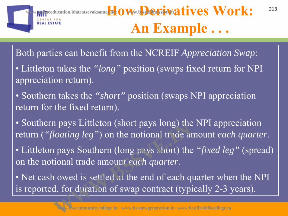
How Derivatives Work:An Example . . .
Both parties can benefit from the NCREIF Appreciation Swap:• Littleton takes the “long” position (swaps fixed return for NPI appreciation return).• Southern takes the “short” position (swaps NPI appreciation return for the fixed return).• Southern pays Littleton (short pays long) the NPI appreciation return (“floating leg”) on the notional trade amount each quarter.• Littleton pays Southern (long pays short) the “fixed leg” (spread) on the notional trade amount each quarter.• Net cash owed is settled at the end of each quarter when the NPI is reported, for duration of swap contract (typically 2-3 years).
www.bsscommunitycollege.in www.bssnewgeneration.in www.bsslifeskillscollege.in
213www.onlineeducation.bharatsevaksamaj.net www.bssskillmission.in
WWW.BSSVE.IN

Suppose Littleton & Southern agree on a two year contract to trade a “notional”amount of $100 million at the end of 2005, with a “fixed leg” (spread) of 100bps:• No cash changes hands at end of 2005Q4.• Suppose 2006Q1 NPI appreciation return is 2.5%, then:
• Southern owes Littleton (short owes long) .025*$100 = $2,500,000;• Littleton owes Southern (long owes short) .01*$100 = $1,000,000;• They settle net cash flow: Southern pays Littleton $1,500,000.
• Suppose 2006Q2 NPI appreciation return is then negative 1.0%:• Southern owes Littleton -.01*$100 = -$1,000,000 (i.e., Littleton owes Southern $1,000,000);• Littleton still owes Southern another $1,000,000 on the fixed spread (as always);• They settle net cash flow: Littleton pays southern $2,000,000.
• This process continues through 2007Q4.
How Derivatives Work:An Example . . .
www.bsscommunitycollege.in www.bssnewgeneration.in www.bsslifeskillscollege.in
214www.onlineeducation.bharatsevaksamaj.net www.bssskillmission.in
WWW.BSSVE.IN

How Derivatives Work:An Example . . .
Portfolio risk impact on Littleton (long position):
• Gains risk effect of $100 million worth of real estate investment;
• Loses risk effect of $100 million worth of riskfree bond investment.
i.e.: They’ve “swapped” $100 million of riskfree bond risk for $100 million of private R.E. risk (because virtually all of the quarterly risk in R.E. investment is in the appreciation return).
www.bsscommunitycollege.in www.bssnewgeneration.in www.bsslifeskillscollege.in
215www.onlineeducation.bharatsevaksamaj.net www.bssskillmission.in
WWW.BSSVE.IN

How Derivatives Work:An Example . . .
Portfolio risk impact on Southern (short position):
• Gains risk effect of $100 million worth of riskfree bonds;
• Loses risk effect of $100 million worth of private R.E. investment (like NPI).
i.e.: They’ve “swapped” $100 million of real estate risk for $100 million of riskfree bond risk (i.e., they’ve eliminated $100 million worth of R.E. risk exposure, again because virtually all of the quarterly risk in R.E. investment is in the appreciation return, and the fixed spread is riskless).
www.bsscommunitycollege.in www.bssnewgeneration.in www.bsslifeskillscollege.in
216www.onlineeducation.bharatsevaksamaj.net www.bssskillmission.in
WWW.BSSVE.IN

How Derivatives Work:An Example . . .
• Littleton (long position) “covers” their exposure to the fixed spread by holding $100 million of riskfree bonds in their portfolio.
• Southern (short position) “covers” their exposure to the floating leg (NPI appreciation return) by holding $100 million of real estate (similar to NCREIF properties) in their portfolio.
www.bsscommunitycollege.in www.bssnewgeneration.in www.bsslifeskillscollege.in
217www.onlineeducation.bharatsevaksamaj.net www.bssskillmission.in
WWW.BSSVE.IN
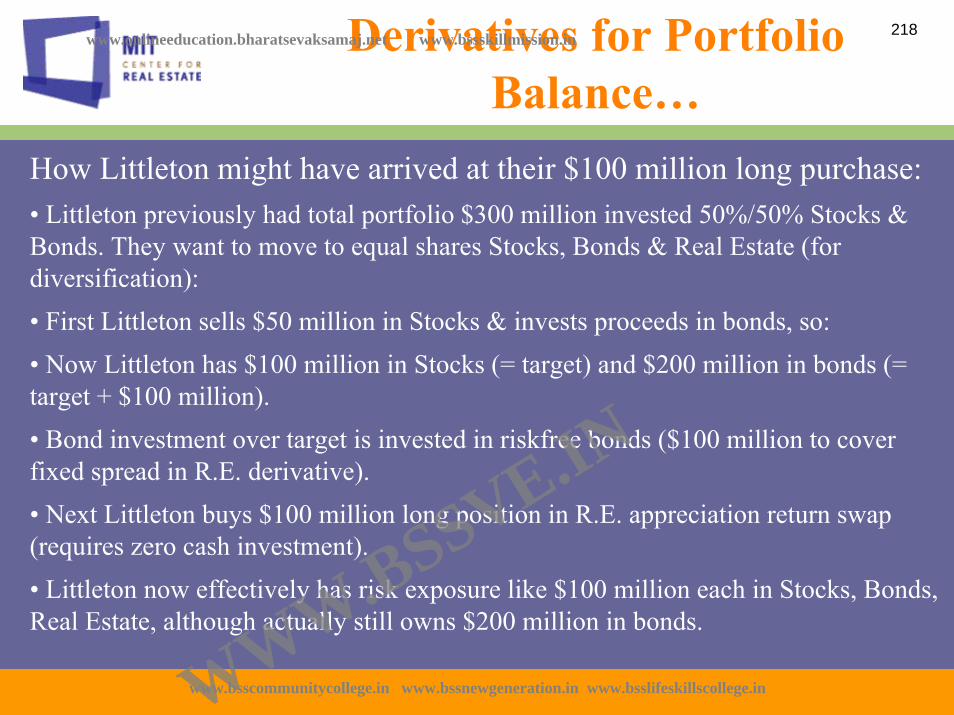
How Littleton might have arrived at their $100 million long purchase:• Littleton previously had total portfolio $300 million invested 50%/50% Stocks & Bonds. They want to move to equal shares Stocks, Bonds & Real Estate (for diversification):• First Littleton sells $50 million in Stocks & invests proceeds in bonds, so:• Now Littleton has $100 million in Stocks (= target) and $200 million in bonds (= target + $100 million).• Bond investment over target is invested in riskfree bonds ($100 million to cover fixed spread in R.E. derivative).• Next Littleton buys $100 million long position in R.E. appreciation return swap (requires zero cash investment).• Littleton now effectively has risk exposure like $100 million each in Stocks, Bonds, Real Estate, although actually still owns $200 million in bonds.
Derivatives for Portfolio Balance…
www.bsscommunitycollege.in www.bssnewgeneration.in www.bsslifeskillscollege.in
218www.onlineeducation.bharatsevaksamaj.net www.bssskillmission.in
WWW.BSSVE.IN

Littleton could accomplish this same result by buying $100 million worth of properties or private R.E. investment funds.However:
• Transaction costs & management fees might be higher than derivative fees.
• Effectively fewer number of properties (even in a fund) would add “noise” and/or “basis risk” compared to derivative that tracks NPI benchmark.
• There might be less liquidity or a longer horizon fixed commitment (less investment flexibility), certainly with direct property investment, possibly with fund investment (depending on type of fund).
Derivatives for Portfolio Balance…
www.bsscommunitycollege.in www.bssnewgeneration.in www.bsslifeskillscollege.in
219www.onlineeducation.bharatsevaksamaj.net www.bssskillmission.in
WWW.BSSVE.IN

Another consideration:
For property returns to be as liquid as derivative returns, property returns must be based on transaction prices.
Derivative returns are based on an appraisal-based index (at least in the case of NPI & IPD), which might have more favorable risk characteristics (due to “smoothing”).(This consideration is better for the long position than the short.)
Derivative Risk vs Property Risk from a Portfolio Perspective
www.bsscommunitycollege.in www.bssnewgeneration.in www.bsslifeskillscollege.in
220www.onlineeducation.bharatsevaksamaj.net www.bssskillmission.in
WWW.BSSVE.IN

How Southern might have arrived at their $100 million short purchase:Previous Southern Portfolio:Stocks: $3333 M (55%)Bonds: $1818 M (30%)R.E.: $ 909 M (15%)Total: $6060 M (100%)
After 20% Stock Crash, Portfolio:Stocks: $2667 M (49%): Δ - $666 MBonds: $1818 M (34%): Δ 0R.E.: $ 909 M (17%): Δ 0 Total: $5394 M (100%): Δ - $666 M
Southern is now below-target in Stocks, above in bonds & R.E. (aka “denominator effect”…) Can correct (rebalance) by:
Purchase (Sale):Stocks: $300 M (11% of previous)Bonds: ($200 M) (11% of previous) R.E.: ($100 M) (11% of previous) Total Net:$ 0 M (0% of previous)
New Portfolio:Stocks: $2667 + 300 = 2967 M (55%)Bonds: $1818 - 200 = 1618 M (30%)R.E.: $ 909 - 100 = 809 M (15%) Total: $5394 + 0 = 5394 M (100%)
Southern can accomplish this by . . .
Derivatives for Portfolio Balance…
www.bsscommunitycollege.in www.bssnewgeneration.in www.bsslifeskillscollege.in
221www.onlineeducation.bharatsevaksamaj.net www.bssskillmission.in
WWW.BSSVE.IN

Southern can accomplish the above by: • Short $100 M R.E. Derivative (0 cash flow);• Cover R.E. short by “earmarking” $100 M worth of R.E. (like NCREIF) to cover floating leg (R.E. appreciation), thereby reducing R.E. risk exposure to $809 M;• Short $100 riskless bonds (T-Bond futures mkt) (+$100 M cash flow), covered by R.E. Derivative fixed spread, so no impact on portfolio risk exposure;• Sell $200 M bonds (+$200 M cash flow), reducing bond exposure to $1618 M;• Use resulting +$300 M cash flow to purchase stocks, bringing exposure to $2967 M.
Without having to actually sell any properties.
Purchase (Sale):Stocks: $300 M (11% of previous)Bonds: ($200 M) (11% of previous) R.E.: ($100 M) (11% of previous) Total Net:$ 0 M (0% of previous)
New Portfolio:Stocks: $2667 + 300 = 2967 M (55%)Bonds: $1818 - 200 = 1618 M (30%)R.E.: $ 909 - 100 = 809 M (15%) Total: $5394 + 0 = 5394 M (100%)
Derivatives for Portfolio Balance…
www.bsscommunitycollege.in www.bssnewgeneration.in www.bsslifeskillscollege.in
222www.onlineeducation.bharatsevaksamaj.net www.bssskillmission.in
WWW.BSSVE.IN

Southern could take a more traditional approach of simply borrowing an incremental $100 million against their R.E. portfolio.
However:• Covenants or restrictions may prevent such borrowing;
• Borrowing transaction costs and fees may exceed those of derivative;
• Interest rates may make borrowing NPV < 0 transaction for tax-exempt investor (marginal borrower in debt mkt is taxed);
• And anyway this will not actually produce the target risk & return allocation…
Derivatives for Portfolio Balance…
www.bsscommunitycollege.in www.bssnewgeneration.in www.bsslifeskillscollege.in
223www.onlineeducation.bharatsevaksamaj.net www.bssskillmission.in
WWW.BSSVE.IN

New Portfolio:Stocks: Use proceeds to buy stock: $2667 + 300 = 2967 M (55%)Bonds: Sell $200 M worth: $1818 - 300 = 1518 M (28%)R.E.: Borrow $100 M like shorting bonds: $ 909 - 0 = 909 M (17%) Total: $5394 + 0 = 5394 M (100%)
The result of simply borrowing $100 million against their R.E. portfolio may reduce the real estate equity on Southern’s books to $809 million, but it increases the leverage of their real estate, thereby retaining the risk and return impact of the full $909 million real estate asset holding in the portfolio.
The borrowing is like “shorting” bonds, thereby negating another $100 million of bond investment in the portfolio risk/return profile, resulting in the following effective portfolio allocation:
The only way to produce the target result without the use of the derivative is by actually selling $100 million worth of Southern’s R.E. properties.
Derivatives for Portfolio Balance…
www.bsscommunitycollege.in www.bssnewgeneration.in www.bsslifeskillscollege.in
224www.onlineeducation.bharatsevaksamaj.net www.bssskillmission.in
WWW.BSSVE.IN

Other Derivative Products
The Property Sector Swap
Swap total return of one NPI sub-index for total return of another plus/minus a fixed leg (that might equal zero).
Useful for portfolio rebalancing.
To better match benchmark (reduce a type of systematic “basis risk”).
To “speculate” (make a bet) on one sector where you feel you have superior knowledge.
www.bsscommunitycollege.in www.bssnewgeneration.in www.bsslifeskillscollege.in
225www.onlineeducation.bharatsevaksamaj.net www.bssskillmission.in
WWW.BSSVE.IN

Derivatives for Hedging & Speculation…
Previous example showed use of derivative for portfolio balancing or target allocation purposes.
There is another major use for derivatives:
Speculation & Hedging…
www.bsscommunitycollege.in www.bssnewgeneration.in www.bsslifeskillscollege.in
226www.onlineeducation.bharatsevaksamaj.net www.bssskillmission.in
WWW.BSSVE.IN

Using Derivatives to Make Money in a Down Market…
Suppose you think the real estate market (& NPI) is headed down.
You stand to lose money, even though you are a good real estate asset manager.
You can use the short position in the NPI appreciation or total return future to continue to make money in the down market…
www.bsscommunitycollege.in www.bssnewgeneration.in www.bsslifeskillscollege.in
227www.onlineeducation.bharatsevaksamaj.net www.bssskillmission.in
WWW.BSSVE.IN
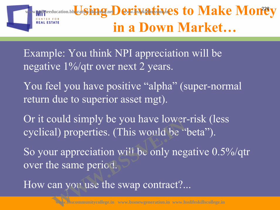
Example: You think NPI appreciation will be negative 1%/qtr over next 2 years.
You feel you have positive “alpha” (super-normal return due to superior asset mgt).
Or it could simply be you have lower-risk (less cyclical) properties. (This would be “beta”).
So your appreciation will be only negative 0.5%/qtr over the same period.
How can you use the swap contract?...
Using Derivatives to Make Money in a Down Market…
www.bsscommunitycollege.in www.bssnewgeneration.in www.bsslifeskillscollege.in
228www.onlineeducation.bharatsevaksamaj.net www.bssskillmission.in
WWW.BSSVE.IN

Say you short $100 million of NPI appreciation futures.
If your expectations are born out, you will receive $1 million per qtr from the derivative, plus the fixed spread (which however will probably be negative, hence paid by you).
You lose only about $500,000 per qtr on your property revaluations, leaving you net positive by $500,000 before counting the fixed spread.
If the fixed spread is greater than negative 50 basis-points, you will make money on property appreciation in a down market!
(You of course also still have your properties’ cash yield.)
Using Derivatives to Make Money in a Down Market…
www.bsscommunitycollege.in www.bssnewgeneration.in www.bsslifeskillscollege.in
229www.onlineeducation.bharatsevaksamaj.net www.bssskillmission.in
WWW.BSSVE.IN
Even if you don’t have positive “alpha”, shorting the appreciation derivative “hedges” the down side of the real estate market.
Even if you don’t fully cover your property position, you can reduce downside volatility by shorting the appreciation swap.
This is like:
Property Market InsuranceIf you have it when the market is headed down, you will likely “beat the benchmark”, and you will beat the performance of other portfolio managers who haven’t hedged.
Using Derivatives to Make Money in a Down Market…
www.bsscommunitycollege.in www.bssnewgeneration.in www.bsslifeskillscollege.in
230www.onlineeducation.bharatsevaksamaj.net www.bssskillmission.in
WWW.BSSVE.IN

Pricing the appreciation swap…
There are two major approaches to analyzing the pricing (or valuation) of the real estate index swap:
• Arbitrage Analysis• Equilibrium Analysis
The two approaches give identical results when the underlying index is always valued at the equilibrium (liquid market) value of its constituent properties.There is also a useful methodology for valuing any swap contract:
• Certainty Equivalence DCF Analysis (CEQ)CEQ valuation is based on equilibrium analysis, but gives results identical to both arbitrage and equilibrium analysis when the underlying index is at equilibrium value.
www.bsscommunitycollege.in www.bssnewgeneration.in www.bsslifeskillscollege.in
231www.onlineeducation.bharatsevaksamaj.net www.bssskillmission.in
WWW.BSSVE.IN

First consider an “arbitrage analysis” . . .
• Suppose it were possible to hold and efficiently trade long andshort positions in the NPI directly (a so-called “spot market” for the NPI), such that:
• Possible to construct a riskless hedge between the underlying asset and the swap contract:
• Then we could derive a pricing relationship like the classical “Futures-Spot Parity Theorem” . . .
(Aside note: This implies that the index must itself directly reflect equilibrium price and return
expectations.)
We’ll come back to this point later…
Arbitrage Analysis . . .
www.bsscommunitycollege.in www.bssnewgeneration.in www.bsslifeskillscollege.in
232www.onlineeducation.bharatsevaksamaj.net www.bssskillmission.in
WWW.BSSVE.IN

Let:• Vt = Value level of the underlying appreciation index at end of period t.
• E[y] = Expected income return of the underlying index (assumed constant & riskless).*
• rf = Riskfree interest rate (e.g., LIBOR).
• F = Fixed leg (spread) paid from long to short position (in percent of notional value).
The “price” of the swap contract is given by F, the value of the agreed-upon fixed spread.
F can be derived by arbitrage analysis as follows . . .
Arbitrage Analysis . . .
www.bsscommunitycollege.in www.bssnewgeneration.in www.bsslifeskillscollege.in
233www.onlineeducation.bharatsevaksamaj.net www.bssskillmission.in
WWW.BSSVE.IN

Cash Flow Today(t)
Cash Flow End of Qtr(t+1)
Cash Flow End of Qtr(t+2)
Short position in Index +Vt -gt+1Vt - E[y]Vt -gt+2 Vt - E[y]Vt - Vt
Invest risklessly zero-coupon
-Vt / (1+rf)2 0 +Vt
Long position in appreciation swap
0 +gt+1Vt - FVt +gt+2Vt - FVt
Hedge Portfolio = Sum +(1-1/(1+rf)2)Vt -(F+E[y])Vt -(F+E[y])Vt
riskless riskless
Consider a 2-period appreciation swap.Construct a riskless hedge as follows:
www.bsscommunitycollege.in www.bssnewgeneration.in www.bsslifeskillscollege.in
234www.onlineeducation.bharatsevaksamaj.net www.bssskillmission.in
WWW.BSSVE.IN

Cash Flow Today(t)
Cash Flow End of Qtr(t+1)
Cash Flow End of Qtr(t+2)
Long position in NPI -Vt gt+1Vt + E[y]Vt gt+2 Vt + E[y]Vt + Vt
Borrow risklessly zero-coupon
+Vt / (1+rf)2 0 -Vt
Short position in appreciation swap
0 -gt+1Vt + FVt -gt+2Vt + FVt
Hedge Portfolio = Sum -(1-1/(1+rf)2)Vt (F+E[y])Vt (F+E[y])Vt
riskless riskless
Or on the other side, the riskless hedge for the short…
www.bsscommunitycollege.in www.bssnewgeneration.in www.bsslifeskillscollege.in
235www.onlineeducation.bharatsevaksamaj.net www.bssskillmission.in
WWW.BSSVE.IN

Suppose you pay a cash price Ct at time t for the long position in the swap.
You can construct the hedge described previously by shorting the index and investing in a riskless zero-coupon bond for a net cash flow at time t of: (1-1/(1+rf)2)Vt , and thereby convert your future cash flow stream into a risklessone of -(F + E[y])V0 each future period.
Thus, including the Ct cost of the swap, the NPV of your transaction at time t is:
Consider a 2-period appreciation swap.Construct a riskless hedge as follows:
( )( ) ( )
( )200
02 1][
1][
111)(
fft
f rVyEF
rVyEFCV
rlongNPV
++
−+
+−−⎟
⎟⎠
⎞⎜⎜⎝
⎛
+−=
Since in fact the swap is purchased for zero net cash up-front at time t, Ct = 0, and the NPV of the long position in the appreciation swap is:
( )( ) ( )
( )200
02 1][
1][
111)(
fff rVyEF
rVyEFV
rlongNPV
++
−+
+−⎟
⎟⎠
⎞⎜⎜⎝
⎛
+−=
www.bsscommunitycollege.in www.bssnewgeneration.in www.bsslifeskillscollege.in
236www.onlineeducation.bharatsevaksamaj.net www.bssskillmission.in
WWW.BSSVE.IN
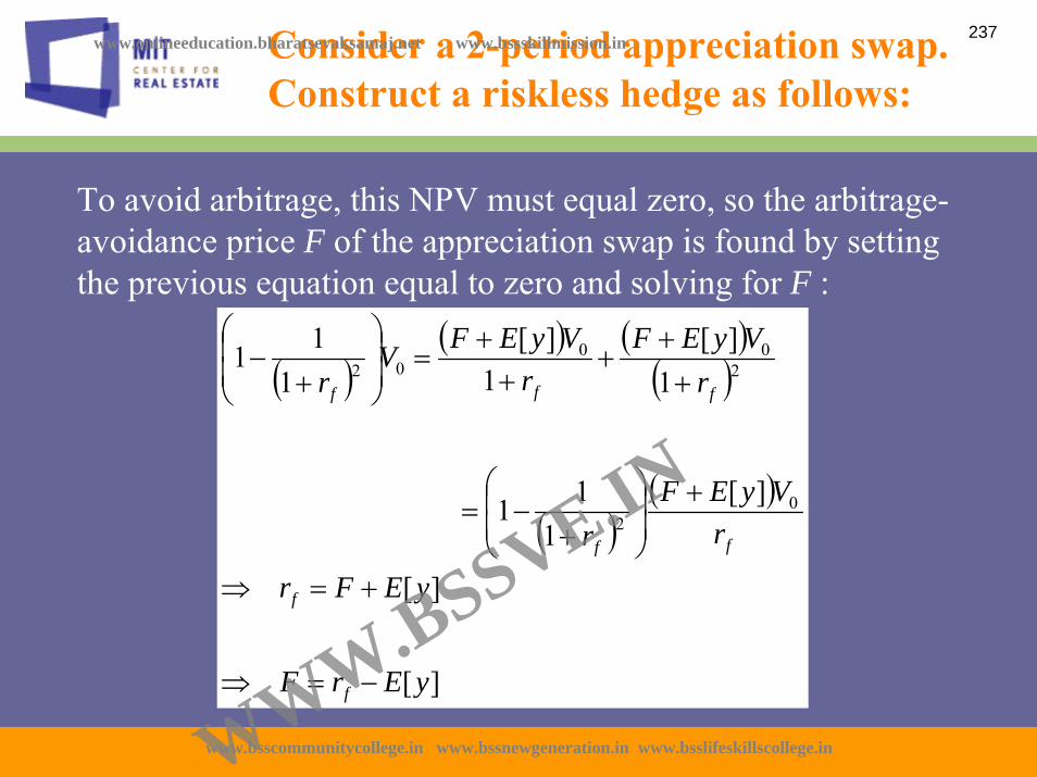
To avoid arbitrage, this NPV must equal zero, so the arbitrage-avoidance price F of the appreciation swap is found by setting the previous equation equal to zero and solving for F :
Consider a 2-period appreciation swap.Construct a riskless hedge as follows:
( )( ) ( )
( )
( )( )
][
][
][1
11
1][
1][
111
02
200
02
yErF
yEFr
rVyEF
r
rVyEF
rVyEFV
r
f
f
ff
fff
−=⇒
+=⇒
+⎟⎟⎠
⎞⎜⎜⎝
⎛
+−=
++
++
+=⎟
⎟⎠
⎞⎜⎜⎝
⎛
+−
www.bsscommunitycollege.in www.bssnewgeneration.in www.bsslifeskillscollege.in
237www.onlineeducation.bharatsevaksamaj.net www.bssskillmission.in
WWW.BSSVE.IN

In general, the price F is given by the following equation:
Extension to a T-period swap . . .
F = rf – E[y]
( )( ) ( )
( )
( )( )
.,][
][
][1
11
1][
1][
111
0
000
TanyyErF
yEFr
rVyEF
r
rVyEF
rVyEFV
r
f
f
fT
f
Tff
Tf
−=⇒
+=⇒
+⎟⎟⎠
⎞⎜⎜⎝
⎛
+−=
++
+++
+=⎟
⎟⎠
⎞⎜⎜⎝
⎛
+− L
www.bsscommunitycollege.in www.bssnewgeneration.in www.bsslifeskillscollege.in
238www.onlineeducation.bharatsevaksamaj.net www.bssskillmission.in
WWW.BSSVE.IN

The fixed spread (F ), price of the appreciation swap, equals the riskfree interest rate minus the real estate income return.
Arbitrage Analysis . . .
Let: E[RPV] = E[rV] – rf = Real Estate (index) Risk PremiumE[g] = Real Estate Expected Appreciation RateE[y] = E[rV] – E[g] = Real Estate Income Return (constant)
Short position first buys the notional amount of real estate and receives expected total return of:
E[rV] = rf + E[RPV] = E[g] + E[y]But then swaps gt for F (replaces gt with F) during the contract, thereby eliminating all risk during that time, hence eliminates any need for E[RPV], giving a required expected return of: F + E[y] = rf , which implies:
F = rf - E[y]Note that this is independent of Er *
www.bsscommunitycollege.in www.bssnewgeneration.in www.bsslifeskillscollege.in
239www.onlineeducation.bharatsevaksamaj.net www.bssskillmission.in
WWW.BSSVE.IN
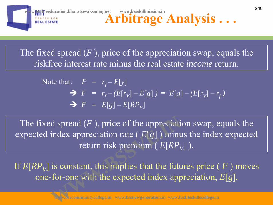
The fixed spread (F ), price of the appreciation swap, equals the riskfree interest rate minus the real estate income return.
Arbitrage Analysis . . .
Note that: F = rf – E[y]F = rf – (E[rV] – E[g] ) = E[g] – (E[rV] – rf )F = E[g] – E[RPV]
The fixed spread (F ), price of the appreciation swap, equals the expected index appreciation rate ( E[g] ) minus the index expected
return risk premium ( E[RPV] ).
If E[RPV] is constant, this implies that the futures price ( F ) moves one-for-one with the expected index appreciation, E[g].
www.bsscommunitycollege.in www.bssnewgeneration.in www.bsslifeskillscollege.in
240www.onlineeducation.bharatsevaksamaj.net www.bssskillmission.in
WWW.BSSVE.IN

Arbitrage Analysis . . .
F = rf – E[y]F = E[g] – E[RPV]
If E[RPV] is constant, this implies that the futures price ( F ) moves one-for-one with the expected index appreciation, E[g].
However, it is important to note that:• As long as the underlying index is priced at its equilibrium value (which it would have to be if we could really use it to construct arbitrages),• F will not necessarily or primarily reflect E[g], but rather:• The equilibrium swap price will primarily reflect interest rates and real estate income returns, according to: F = rf – E[y]. In other words:• If the index is priced at equilibrium, changes over time in E[g] may largely reflect corresponding changes in the market’s equilibrium E[RPV] requirement for real estate, except as reflected in changes in rf – E[y].
www.bsscommunitycollege.in www.bssnewgeneration.in www.bsslifeskillscollege.in
241www.onlineeducation.bharatsevaksamaj.net www.bssskillmission.in
WWW.BSSVE.IN

Arbitrage Analysis . . .
The complete arbitrage valuation formula for the t-period appreciation swap:
( )( ) ( )
( )
( )( )
( )0
0
000
][1,
][11
11
1][
1][
111)(
Vr
yEFTfor
Vr
yEFr
rVyEF
rVyEFV
rlongNPV
f
fT
f
Tff
Tf
⎟⎟⎠
⎞⎜⎜⎝
⎛ +−=∞=
⎟⎟⎠
⎞⎜⎜⎝
⎛ +−⎟
⎟⎠
⎞⎜⎜⎝
⎛
+−=
++
−−+
+−⎟
⎟⎠
⎞⎜⎜⎝
⎛
+−= L
The NPV of the short position is just the negative of the above.Note: F should include impact of fees.
E[y] can be equivalently expressed as: E[rV] – E[g](Caution: This assumes V0 is an equilibrium value: no “index lag”.)
www.bsscommunitycollege.in www.bssnewgeneration.in www.bsslifeskillscollege.in
242www.onlineeducation.bharatsevaksamaj.net www.bssskillmission.in
WWW.BSSVE.IN

Cash Flow Today(t)
Cash Flow End of Qtr(t+1)
Cash Flow End of Qtr(t+2)
Long position in NPI -Vt rt+1Vt rt+2 Vt + Vt
Borrow risklessly zero-coupon
+Vt / (1+rf)2 0 -Vt
Short position in total return swap
0 -rt+1Vt + FVt -rt+2Vt + FVt
Hedge Portfolio = Sum -(1-1/(1+rf)2)Vt FVt FVt
riskless riskless
For total return swap, the riskless hedge for the short…
www.bsscommunitycollege.in www.bssnewgeneration.in www.bsslifeskillscollege.in
243www.onlineeducation.bharatsevaksamaj.net www.bssskillmission.in
WWW.BSSVE.IN

Suppose you pay a cash price Ct at time t for the short position in the swap.
You can construct the hedge described previously by buying the index and risklessly borrowing Vt/(1+rf)2 zero-coupon for 2 periods, for a net cash flow at time t of: -(1-1/(1+rf)2)Vt , and thereby convert your future cash flow stream into a riskless one of FVt each future period.
Thus, including the Ct cost of the swap, the NPV of your transaction at time t is:
Consider a 2-period total return swap.Construct a riskless hedge as follows:
( ) ( )202 11111)(
f
t
f
tt
f rFV
rFVCV
rshortNPV
+−
++−⎟
⎟⎠
⎞⎜⎜⎝
⎛
+−−=
Since in fact the swap is purchased for zero net cash up-front at time t, Ct = 0, and the NPV of the short position in the total return swap is:
( ) ( )22 11111)(
f
t
f
tt
f rFV
rFVV
rshortNPV
+−
+−⎟
⎟⎠
⎞⎜⎜⎝
⎛
+−−=
www.bsscommunitycollege.in www.bssnewgeneration.in www.bsslifeskillscollege.in
244www.onlineeducation.bharatsevaksamaj.net www.bssskillmission.in
WWW.BSSVE.IN

To avoid arbitrage, this NPV must equal zero, so the arbitrage-avoidance price F of the total return swap is found by setting the previous equation equal to zero and solving for F :
Consider a 2-period total return swap.Construct a riskless hedge as follows:
( ) ( )
( )f
f
t
f
f
t
f
tt
f
rF
rFV
r
rFV
rFVV
r
=⇒
⎟⎟⎠
⎞⎜⎜⎝
⎛
+−=
++
+=⎟
⎟⎠
⎞⎜⎜⎝
⎛
+−
2
22
111
11111
www.bsscommunitycollege.in www.bssnewgeneration.in www.bsslifeskillscollege.in
245www.onlineeducation.bharatsevaksamaj.net www.bssskillmission.in
WWW.BSSVE.IN

Equilibrium Analysis . . .
In real estate we cannot construct the arbitrage, because we cannot directly trade the underlying index.
However, the arbitrage analysis gives a pricing result that equates the expected total return risk premium per unit of risk within and across the relevant asset markets: so-called “linear pricing”…
rfRisk
E[r]
E[RP]
This is a characteristic of equilibrium pricing, which may also be viewed as normative (i.e., “fair” ) pricing.
www.bsscommunitycollege.in www.bssnewgeneration.in www.bsslifeskillscollege.in
246www.onlineeducation.bharatsevaksamaj.net www.bssskillmission.in
WWW.BSSVE.IN

From the Perspective of the Covered Long Position…
Littleton’s expected overall net return is:
NPI Appreciation Return (EL[gNPI]), minus the Fixed Spread (F ), plus the riskfree rate (rf ) that they receive on their covering bond investment.
Littleton’s overall net risk exposure is that of the NPI:
Because almost all return risk is in the appreciation return component.
Therefore, Littleton requires:
EL[gNPI] – F + rf ≥ rf + E[RPNPI]
www.bsscommunitycollege.in www.bssnewgeneration.in www.bsslifeskillscollege.in
247www.onlineeducation.bharatsevaksamaj.net www.bssskillmission.in
WWW.BSSVE.IN
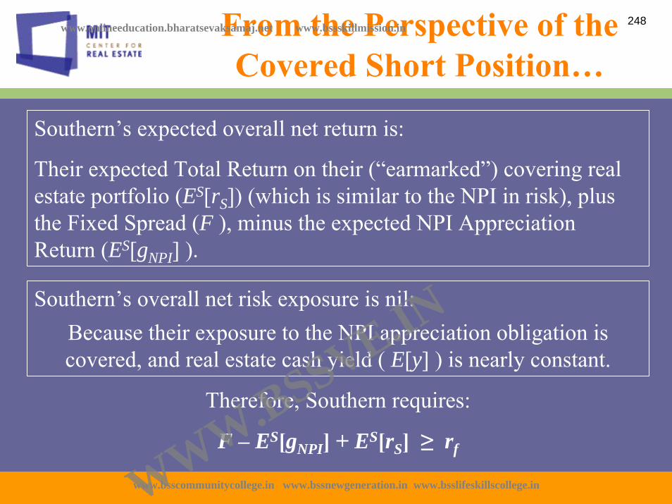
From the Perspective of the Covered Short Position…
Southern’s expected overall net return is:
Their expected Total Return on their (“earmarked”) covering real estate portfolio (ES[rS]) (which is similar to the NPI in risk), plus the Fixed Spread (F ), minus the expected NPI Appreciation Return (ES[gNPI] ).
Southern’s overall net risk exposure is nil:Because their exposure to the NPI appreciation obligation is covered, and real estate cash yield ( E[y] ) is nearly constant.
Therefore, Southern requires:
F – ES[gNPI] + ES[rS] ≥ rf
www.bsscommunitycollege.in www.bssnewgeneration.in www.bsslifeskillscollege.in
248www.onlineeducation.bharatsevaksamaj.net www.bssskillmission.in
WWW.BSSVE.IN

Putting the two previous pricing conditions from each side together, we have the following feasible pricing range for F :
rf – ES[rS] + ES[gNPI] ≤ F ≤ EL[gNPI] – E[RPNPI]
Equilibrium Analysis . . .
If all parties have the same expectations, the above pricing condition becomes:
rf – E[rNPI] + E[gNPI] ≤ F ≤ E[gNPI] – E[RPNPI]
rf – (rf + E[RPNPI]) + E[gNPI] ≤ F ≤ E[gNPI] – E[RPNPI]
–E[RPNPI] + E[gNPI] ≤ F ≤ E[gNPI] – E[RPNPI]
F = E[gNPI] – E[RPNPI] = rf – E[yNPI]
which is the same as the arbitrage-based result*.
www.bsscommunitycollege.in www.bssnewgeneration.in www.bsslifeskillscollege.in
249www.onlineeducation.bharatsevaksamaj.net www.bssskillmission.in
WWW.BSSVE.IN

F = E[gNPI] – E[RPNPI] = rf – E[yNPI]In this derivation we have not assumed that the underlying index is priced at its equilibrium value.
However, if the underlying index is priced at its equilibrium value, then the same observations as before apply to the equilibrium price and valuation of the swap contract. In particular:
Swap price and value are:
• Independent of Index Expected Return E[rV].
• Independent of Index Expected Appreciation E[g].
• Except in both cases as these expectations are reflected in rf – E[y]. (i.e., movements in equilibrium E[g] & E[RPV] may largely cancel.)
• Independent of the Volatility of the underlying Index.
Equilibrium Analysis . . .
www.bsscommunitycollege.in www.bssnewgeneration.in www.bsslifeskillscollege.in
250www.onlineeducation.bharatsevaksamaj.net www.bssskillmission.in
WWW.BSSVE.IN

F = E[gNPI] – E[RPNPI] = rf – E[yNPI]There is an important corollary to this observation:
If real estate swap prices (spreads) are observed to move noticeably with:
• Changes in Index Expected Returns going forward E[rV] , OR
• Changes in Index Expected Appreciation going forward E[g],
• Beyond the movements implied by changes in rf – E[y] ,
Then:
The underlying index is not priced at equilibrium(e.g., the index value may be lagged behind current property market
equilibrium values due to the effect of appraisal valuation and/or other index construction issues.)
Equilibrium Analysis . . .
www.bsscommunitycollege.in www.bssnewgeneration.in www.bsslifeskillscollege.in
251www.onlineeducation.bharatsevaksamaj.net www.bssskillmission.in
WWW.BSSVE.IN

F = E[gNPI] – E[RPNPI] = rf – E[yNPI]For the appreciation swap this pricing rule will often give a negative value for F (that is, short party pays the fixed spread to the long party). This will almost always be true if the underlying index is priced at its equilibrium value.This is because the appreciation return is only fraction of the total return that is required to compensate investors for bearing real estate investment risk,And the swap long position that bears that risk only receives the appreciation return, not the total return.If the swap contract is written on the total return (E[rNPI]) instead of just the appreciation, we obtain by the same reasoning as above (just substitute E[rNPI] for E[gNPI] in the above):
F = E[rNPI] – E[RPNPI] = rf( rf is of course normally positive.*)
Appreciation vs Total Return Swaps for Fixed Spreads…
www.bsscommunitycollege.in www.bssnewgeneration.in www.bsslifeskillscollege.in
252www.onlineeducation.bharatsevaksamaj.net www.bssskillmission.in
WWW.BSSVE.IN

F = E[gNPI] – E[RPNPI] = rf – E[yNPI]The long-term historical average quarterly return components for the NPI are as follows (1978-2005):
E[gNPI] = 0.46%
E[RPNPI] = 0.90%
rf = 1.51%
E[yNPI] = 1.94%
Which implies a long-term average appreciation price, F of:
Typical Numbers…
F = 0.46% – 0.90% = 1.51% – 1.94% = – 0.43%
www.bsscommunitycollege.in www.bssnewgeneration.in www.bsslifeskillscollege.in
253www.onlineeducation.bharatsevaksamaj.net www.bssskillmission.in
WWW.BSSVE.IN

Equilibrium Analysis . . .
Another corollary:
• If the appreciation swap is priced with a positive spread (F > 0),
• It is a strong signal that the underlying index is under-priced relative to the actual current market value of the real estate it represents:
• Index value below its equilibrium level implies expected near-term future returns to the index above their equilibrium rates.
• This could be due to “index lag” after a recent upsurge in property market value. (e.g., 2006.)
www.bsscommunitycollege.in www.bssnewgeneration.in www.bsslifeskillscollege.in
254www.onlineeducation.bharatsevaksamaj.net www.bssskillmission.in
WWW.BSSVE.IN

Suppose over the period of the contract:
The potential long party expects gNPI will overperform 25 bps/qtr above the general market expectation:
EL[gNPI] = E[gNPI] + 25bps.
The potential short party is relatively bearish:ES[gNPI] = E[gNPI] – 25bps.
Suppose further that the potential short party feels that their own (covering) real estate portfolio will beat the NPI totalreturn by an average of 25bps/qtr (even though it contains the same risk as the NPI, i.e., the excess is “alpha” ):
ES[rS] = ES[rNPI] + 25bps
Effect of Heterogeneous Expectations…
www.bsscommunitycollege.in www.bssnewgeneration.in www.bsslifeskillscollege.in
255www.onlineeducation.bharatsevaksamaj.net www.bssskillmission.in
WWW.BSSVE.IN
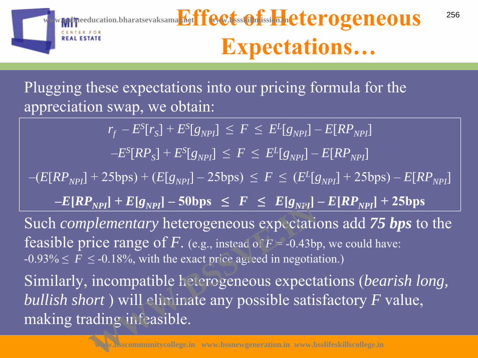
rf – ES[rS] + ES[gNPI] ≤ F ≤ EL[gNPI] – E[RPNPI]
–ES[RPS] + ES[gNPI] ≤ F ≤ EL[gNPI] – E[RPNPI]
–(E[RPNPI] + 25bps) + (E[gNPI] – 25bps) ≤ F ≤ (EL[gNPI] + 25bps) – E[RPNPI]
–E[RPNPI] + E[gNPI] – 50bps ≤ F ≤ E[gNPI] – E[RPNPI] + 25bps
Effect of Heterogeneous Expectations…
Plugging these expectations into our pricing formula for the appreciation swap, we obtain:
Such complementary heterogeneous expectations add 75 bps to the feasible price range of F. (e.g., instead of F = -0.43bp, we could have: -0.93% ≤ F ≤ -0.18%, with the exact price agreed in negotiation.)
Similarly, incompatible heterogeneous expectations (bearish long, bullish short ) will eliminate any possible satisfactory F value, making trading infeasible.
www.bsscommunitycollege.in www.bssnewgeneration.in www.bsslifeskillscollege.in
256www.onlineeducation.bharatsevaksamaj.net www.bssskillmission.in
WWW.BSSVE.IN

Type of Heterogeneity Useful for Trading…
Implication of the fact that the zero-NPV price condition can be expressed in either of two ways:
E[g] – E[RP] OR rf – E[y]
Apart from “alpha” considerations, in order to obtain complementary (overlapping) price requirements, we require:
Heterogeneity in gNPI expectations that are not canceled out by heterogeneity in RPNPI expectations. This requires:
Offsetting E[gNPI] & E[yNPI] expectations.e.g.: If the long party believes that NPI appreciation will be 1%/year higher than average it must also believe that NPI income yields will be 1%/year lower than average.
www.bsscommunitycollege.in www.bssnewgeneration.in www.bsslifeskillscollege.in
257www.onlineeducation.bharatsevaksamaj.net www.bssskillmission.in
WWW.BSSVE.IN

rf – ES[rS] + ES[gNPI] + f ≤ F ≤ EL[gNPI] – E[RPNPI] – f
Effect of Transaction Fees…
Transaction fees narrow the feasible trading range.
If the fees are f basis-points of notional value per period (charged to each party), then the feasible pricing range becomes:
This would seem to require complementary heterogeneous expectations in order to allow any feasible trading range.
However, . . .
EL[gNPI] – ES[gNPI] + ES[rS] – E[RPNPI] – rf
Fees charged to both parties together must be less than:
www.bsscommunitycollege.in www.bssnewgeneration.in www.bsslifeskillscollege.in
258www.onlineeducation.bharatsevaksamaj.net www.bssskillmission.in
WWW.BSSVE.IN

Effect of Transaction Fees…
The above analysis ignores the savings of transactions costs, investment management fees, and other advantages of using derivatives versus traditional methods of accomplishing the portfolio balancing or hedging/speculation objectives underlyingthe short and long positions.
For example, suppose the long party would avoid 20 bp/qtr in investment management and fund fees, and suppose the short partyeffectively saves 10 bp/qtr in costs of borrowing against their portfolio (alternative traditional methods to accomplish portfolio balancing objectives).
Then even with homogeneous expectations, there exists 30 bp/qtr of savings that can be split among the two parties and the brokers and investment banking fees of the derivative process.
www.bsscommunitycollege.in www.bssnewgeneration.in www.bsslifeskillscollege.in
259www.onlineeducation.bharatsevaksamaj.net www.bssskillmission.in
WWW.BSSVE.IN
What about predictability in the NPI?…
Appraisal smoothing and stale appraisals (along with true underlying property market sluggishness) give the NPI much more inertia than typical securities indexes, making the NPI relatively smooth and predictable.
Wouldn’t this type of predictability result in an absence of heterogeneous expectations, and thereby an absence of counterparties for trading the derivatives, making a functioningfutures market impossible?
www.bsscommunitycollege.in www.bssnewgeneration.in www.bsslifeskillscollege.in
260www.onlineeducation.bharatsevaksamaj.net www.bssskillmission.in
WWW.BSSVE.IN

What about predictability in the NPI?…
Answer: Not necessarily.As seen in our Littleton & Southern example, derivative traders may have reasons other than speculation for trading derivatives. Heterogeneous expectations may not be necessary.
Predictability in the NPI will simply come out in the equilibrium derivative price, F.
Recall that F is a function of the market participants’ expectations about the future NPI appreciation returns: EL[gNPI] and ES[gNPI].
e.g., if NPI is headed down, then E[gNPI] will be negative, making F more negative than it would otherwise be (meaning the short position must pay the long position more in the fixed leg).
Well-functioning futures markets have long existed for various commodities and financial products whose future price directions are often rather predictable in advance (e.g., corn, wheat, oil, foreign exchange, among others).
www.bsscommunitycollege.in www.bssnewgeneration.in www.bsslifeskillscollege.in
261www.onlineeducation.bharatsevaksamaj.net www.bssskillmission.in
WWW.BSSVE.IN

What about predictability in the NPI?…
Of course, predictability in the NPI means that derivatives traders who don’t want to get taken advantage of must use all the relevant information as skillfully as possible to be educated about what are reasonable expectations of where the NPI is headed.
For example (inter alia ), the MIT transactions-based index (which tends to lead the NPI…)
Roughly speaking: gNPI(yr t) = (1/2)gTBI(yr t-1) + (1/2)gTBI(yr t).
www.bsscommunitycollege.in www.bssnewgeneration.in www.bsslifeskillscollege.in
262www.onlineeducation.bharatsevaksamaj.net www.bssskillmission.in
WWW.BSSVE.IN

What about predictability in the NPI?…
Effect of Index Lag on Swap Pricing and Valuation:Effect of Index Lag on Swap Pricing and Valuation:Index Lag Index will often not be valued at its equilibrium value.That is, realistic expected returns on the index differ in the near-term from long-run equilibrium rates.In such circumstances, the Arbitrage Pricing and Valuation Formula for the swap no longer holds.The zero-NPV pricing condition will still be well approximated by:
F = E[g] – E[RPV]but not by rf – E[y], and only provided that E[RPV] in the above formula reflects the market’s long-run equilibrium risk premium, not the current disequilibrium premium presented by the index (while E[g] reflects the non-equilibrium appreciation in the index).
www.bsscommunitycollege.in www.bssnewgeneration.in www.bsslifeskillscollege.in
263www.onlineeducation.bharatsevaksamaj.net www.bssskillmission.in
WWW.BSSVE.IN

Alternative Pricing Perspectives…
The previous pricing analysis assumed trading by “covered”parties on both sides.Alternative pricing perspectives are possible…Suppose neither party is covered at all, and both view themselves as requiring a return as if they were actually making the notional investment. The resulting pricing condition would be:
rf + ES[gNPI] – E[RPNPI] ≤ F ≤ EL[gNPI] – rf – E[RPNPI]Which implies a feasible pricing range for F of width:
E[gLNPI] – E[gS
NPI] – 2rf
This requires that the long position be substantially more bullish than the short position. But this perspective is not based on an But this perspective is not based on an equilibrium framework . . .equilibrium framework . . .
www.bsscommunitycollege.in www.bssnewgeneration.in www.bsslifeskillscollege.in
264www.onlineeducation.bharatsevaksamaj.net www.bssskillmission.in
WWW.BSSVE.IN

Alternative Pricing Perspectives…
We can analyze equilibrium pricing of the uncovered swap by using certainty-equivalence valuation (CEQ)…Consider a 1-period binomial world;V0 = Current value of the R.E.index & notional amt of swap trade;p = Probability of the “up” move in index next period (real prob)V1
up , V1down = Value of index next period in “up”
or “down” outcomes;g = 1-period appreciation return on index;F = Appreciation swap price (fixed leg) in fraction of notional trade amount.
VV00
VV11upup
VV11downdown
pp
11--pp
VV11upup = = (1 + g(1 + gupup)V)V00
VV11downdown = = (1 + g(1 + gdowndown)V)V00
E[E[VV11] = ] = (1 + E(1 + E[[gg]])V)V00
= [= [p(1+gp(1+gupup)) + (1+ (1--pp))(1+g(1+gdowndown))]]VV00
= [ = [ 11 + + pgpgupup + (1+ (1--pp))ggdowndown ]]VV00
EE[[gg] = ] = pgpgupup + (1+ (1--pp))ggdowndown
www.bsscommunitycollege.in www.bssnewgeneration.in www.bsslifeskillscollege.in
265www.onlineeducation.bharatsevaksamaj.net www.bssskillmission.in
WWW.BSSVE.IN

Alternative Pricing Perspectives…
Cash flow amts for apprec swap long position:Expected CF next period is:
00
CFCF11upup = = ((ggupup –– F)VF)V00
CFCF11downdown = = ((ggdowndown –– F)VF)V00
pp
11--pp
E[E[CFCF11] = [] = [pgpgupup + (1+ (1--pp))ggdowndown ]]VV00 –– FVFV00
= ( = ( EE[[gg] ] –– FF ))VV00
Certainty Equivalent CF next period is:CEQCEQ[[CFCF11] = ] = EE[[CFCF11] ] –– EE[[RPRPVV](](CFCF11
upup –– CFCF11downdown )/()/(VV11
upup//VV00 –– VV11downdown/V/V0 0 ))
= = EE[[CFCF11] ] –– ( ( EE[[rrVV] ] –– rrff )()(ggupup –– ggdowndown )V)V00 / (/ (ggupup –– ggdowndown ))
== EE[[CFCF11] ] –– ( ( EE[[rrVV] ] –– rrff ))VV00
Hence, present value of uncovered swap CF next period is:PVPV[[CFCF11] = [ ] = [ EE[[CFCF11] ] –– ( ( EE[[rrVV] ] –– rrff ))VV00 ] / (1 + ] / (1 + rrff ))
In equilibrium, this must equal the 0 net CF of the trade today:PVPV[[CFCF11] = [ ] = [ EE[[CFCF11] ] –– ( ( EE[[rrVV] ] –– rrff ))VV00 ] / (1 + ] / (1 + rrff ) = ) = 00 . . EE[[CFCF11] = ] = ( ( EE[[rrVV] ] –– rrff ))VV00
www.bsscommunitycollege.in www.bssnewgeneration.in www.bsslifeskillscollege.in
266www.onlineeducation.bharatsevaksamaj.net www.bssskillmission.in
WWW.BSSVE.IN

Alternative Pricing Perspectives…
Thus, we have the equilibrium condition:
00
CFCF11upup = = ((ggupup –– F)VF)V00
CFCF11downdown = = ((ggdowndown –– F)VF)V00
pp
11--pp
EE[[CFCF11] = ] = ( ( EE[[rr] ] –– rrff ))VV00
( ( EE[[gg] ] –– FF ))VV00 = ( = ( EE[[rr] ] –– rrff ))VV00
FF = = rrff + + EE[[gg] ] –– EE[[rr] = ] = EE[[gg] ] –– EE[[RPRP]]
== rrff –– EE[[yy]]
This is the same equilibrium pricing condition that we obtained before:
F = E[g] – E[RP] = rf – E[y]
www.bsscommunitycollege.in www.bssnewgeneration.in www.bsslifeskillscollege.in
267www.onlineeducation.bharatsevaksamaj.net www.bssskillmission.in
WWW.BSSVE.IN

( )( ) ( )( )
( )Tf
Tf
TV
VT
Tf
TT r
rrErSTDCSTDCE
rCCEQCPV
+
+−+⎟⎟⎠
⎞⎜⎜⎝
⎛±
=+
=1
1][1][][][
1][][ 0
100
0
Certainty Equivalence Valuation of Derivatives…
In general, we can use certainty-equivalence discounting to evaluate the swap with heterogeneous expectations, and whether or not the underlying index is valued at its equilibrium level…The general certainty equivalence valuation (CEQ) formula for valuing a derivative cash flow is as follows:Let: Ct = The derivative value (cash flow) t periods hence,
E[rV] = Equilibrium expected total return on underlying asset (per period).
Then the Certainty Equivalence PV formula is as follows for a single sum T periods in the future, with risk accumulation throughout T ):*
The risk adjustment is subtracted for long positions, added for shorts.
www.bsscommunitycollege.in www.bssnewgeneration.in www.bsslifeskillscollege.in
268www.onlineeducation.bharatsevaksamaj.net www.bssskillmission.in
WWW.BSSVE.IN

Certainty Equivalence Valuation of Derivatives…
For the index swap, the CEQ valuation formula for a given future cash flow of the swap t periods in the future (Ct) with current value of the underlying index (= notional amount of trade) V0 is:
( )( )
( )
( )
( )
( )( ) .1
][][
1][
][][][
1][][][][
1][][
00
00
00
0
tf
Vt
tf
V
VVt
tf
V
tVt
tf
tt
rVRPECE
rrSTD
VrSTDRPECE
rrSTDCSTDRPECE
rCCEQCPV
+±
=
+
⎟⎟⎠
⎞⎜⎜⎝
⎛±
=
+
⎟⎟⎠
⎞⎜⎜⎝
⎛±
=+
=
There is only 1 period of risk accumulation (just prior to the cash flow), because the cash flow is based solely on the index return in period ttimes a notional amount that is fixed up front at time 0. Hence, the risk adjustment in the numerator is for just one period.
Where the risk adjustment in the numerator is subtracted for long positions and added for short positions (negative correl betwswap & index).
where E[RPV] is the mkt equilibrium risk premium.
www.bsscommunitycollege.in www.bssnewgeneration.in www.bsslifeskillscollege.in
269www.onlineeducation.bharatsevaksamaj.net www.bssskillmission.in
WWW.BSSVE.IN

Consider a 1-period example with F = -60bp and the following expectations:Long Perspective: rf = 0.75% /qtr Short Perspective:EL[rNPI] = 2.00% /qtr ES[rNPI] = 2.00% /qtrEL[gNPI] = 0.75% /qtr ES[gNPI] = 0.55% /qtrEL[RPNPI] = 1.25% /qtr ES[RPNPI] = 1.25% /qtrEL[C1] = (0.0075 – (-0.0060))$100 ES[C1] = (-0.0055 + (-0.0060))$100
= $0.75 + $0.60 = $1.35. = -$0.55 – $0.60 = -$1.15.Applying the certainty equivalence DCF valuation formula:
Certainty Equivalence Valuation of Derivatives…
( ) ( ) 0993.0$0075.1
25.1$35.1$0075.1
100$0125.35.1$][][][ 110 =
−=
−=
−=
f
VtL
tL
RVRPECECPV
( ) ( ) 0993.0$0075.1
25.1$15.1$0075.1
100$0125.15.1$][][][ 110 =
+−=
+−=
−=
f
VtS
tS
RVRPECECPV
Because of heterogeneous expectations,The trade allows both sides to face a positive NPV ex ante.
www.bsscommunitycollege.in www.bssnewgeneration.in www.bsslifeskillscollege.in
270www.onlineeducation.bharatsevaksamaj.net www.bssskillmission.in
WWW.BSSVE.IN

Certainty Equivalence Valuation of Derivatives…
PV[C] = CEQ[C] / (1+rf) = $0.10 / 1.0075 = $0.0993.Even though the expected cash flow is $1.35 for the long position, -$1.15 for the short position, the certainty equivalent cash flow is only $0.10 in both cases. The certainty-equivalence operation reverses the sign of the short position cash flow expectation, because the risk in the short position is negative the risk in the underlying index, because the two are perfectly negatively correlated.
( ) ( ) 0993.0$0075.1
25.1$35.1$0075.1
100$0125.35.1$][][][ 110 =
−=
−=
−=
f
VtL
tL
RVRPECECPV
( ) ( ) 0993.0$0075.1
25.1$15.1$0075.1
100$0125.15.1$][][][ 110 =
+−=
+−=
−=
f
VtS
tS
RVRPECECPV
Note that you should always employ the market equilibrium risk premium for the underlying index.
www.bsscommunitycollege.in www.bssnewgeneration.in www.bsslifeskillscollege.in
271www.onlineeducation.bharatsevaksamaj.net www.bssskillmission.in
WWW.BSSVE.IN

NPVL = +$0.0993.Same answer as before.
(But this formula only works if the underlying index is in equilibrium.)
Same thing using the arbitrage formula…
See downloadable Excel® file example on book CD
( )( )
( )0993.0$100$*13333.0*00744.0
100$0075.
0125.0060.10075.1
11
11
11)(
1
0
==
⎟⎠⎞
⎜⎝⎛ +−−⎟⎟
⎠
⎞⎜⎜⎝
⎛−=
⎟⎟⎠
⎞⎜⎜⎝
⎛ +−⎟
⎟⎠
⎞⎜⎜⎝
⎛
+−= NPI
rEyF
rlongNPV
fT
f
NPVS = +$0.0993.
Given the same conditions as before with F = -0.60%:rf = 0.75% /qtr
EL[rNPI] = 2.00% /qtr ES[rNPI] = 2.00% /qtrEL[gNPI] = 0.75% /qtr ES[gNPI] = 0.55% /qtr
Define:EyL = EL[rNPI] – EL[gNPI] = 2% – .75% = 1.25%EyS = ES[rNPI] – ES[gNPI] = 2% – .55% = 1.45%
Applying the arbitrage valuation formula to the $100 notional trade:
( )( )
( )0993.0$100$*13333.0*00744.0
100$10075.
0145.0060.0075.1
11
11
11)(
1
0
==
⎟⎠⎞
⎜⎝⎛ −
+−⎟⎟⎠
⎞⎜⎜⎝
⎛−=
⎟⎟⎠
⎞⎜⎜⎝
⎛−
+⎟⎟⎠
⎞⎜⎜⎝
⎛
+−= NPI
rEyF
rlongNPV
fT
f
www.bsscommunitycollege.in www.bssnewgeneration.in www.bsslifeskillscollege.in
272www.onlineeducation.bharatsevaksamaj.net www.bssskillmission.in
WWW.BSSVE.IN

What are Derivatives?
• A claim whose cash flow and value are derived completely from one or more underlying assets, financial instruments or indices
• Usually involve one of the following:• Futures• Swaps• Options
• Traded on exchanges like CBOT and CME and off-exchange (OTC)
www.bsscommunitycollege.in www.bssnewgeneration.in www.bsslifeskillscollege.in
273www.onlineeducation.bharatsevaksamaj.net www.bssskillmission.in
WWW.BSSVE.IN

Example – Foreign Investor• A foreign investor wants to quickly get exposure to the US
real estate market to diversify into the US but doesn’t have the time and expertise to identify individual properties and be sure he is also diversified within the US.
• They enter into a long position on a two year forwardcontract based on a national real estate index total return. The index is currently at 100. Forecasts for where the index will be in 2 yrs range from 105 to 115 (including cash yield).
• Investor agrees on a forward price of 105 that it will pay at the end of the two years in order to receive a payment based on the actual change in the index.
• The contract pays $500,000 times the index value.• No cash payment is made today although a margin or
bond may be required.
www.bsscommunitycollege.in www.bssnewgeneration.in www.bsslifeskillscollege.in
274www.onlineeducation.bharatsevaksamaj.net www.bssskillmission.in
WWW.BSSVE.IN

Payoff
• Suppose that at the end of the two years the index is 115 (upper end of forecast). The investor will receive$500,000 x (115 -105) = $5 million
• Suppose that at the end of the two years the index is 95 (bad forecast!).
The investor will pay$500,000 x (95 -105) = -$5 million
www.bsscommunitycollege.in www.bssnewgeneration.in www.bsslifeskillscollege.in
275www.onlineeducation.bharatsevaksamaj.net www.bssskillmission.in
WWW.BSSVE.IN

Short Position(This is the “counterparty”, or opposite side: Every
derivative trade requires both a “long” and “short” side to the trade…)
• The short position receives the opposite cash flows in the previous example, receiving $5 million when the index is 95 and paying $5 million when it is 115.
• The short might be a CMBS issuer who wants to hedge its warehouse risk, a hedge fund that believed the low end of the forecast was more likely or an investment manager seeking to “harvest alpha” (explained next).
www.bsscommunitycollege.in www.bssnewgeneration.in www.bsslifeskillscollege.in
276www.onlineeducation.bharatsevaksamaj.net www.bssskillmission.in
WWW.BSSVE.IN

Harvesting “Alpha”A specialized RE asset mgt fund believes it can
purchase properties that consistently out-perform the RE index (with same risk), based on their specialized expertise. They want to harvest the “alpha” from these excess returns whether the market is up or down (which they can’t control, whereas they do control their “alpha”–difference betw their properties vs market).
They purchase $50 million in properties and sell (short) the forward contract on the index used in the previous example.
www.bsscommunitycollege.in www.bssnewgeneration.in www.bsslifeskillscollege.in
277www.onlineeducation.bharatsevaksamaj.net www.bssskillmission.in
WWW.BSSVE.IN

Results when values increase
• Suppose at the end of the two years the real estate fund’s property portfolio increased in value by 20% (including income reinvested in fund). Suppose the total return index rose to 115 over the two years.
Appreciation on portfolio $10,000,000Loss on short futures $5,000,000Net gain $5,000,000
www.bsscommunitycollege.in www.bssnewgeneration.in www.bsslifeskillscollege.in
278www.onlineeducation.bharatsevaksamaj.net www.bssskillmission.in
WWW.BSSVE.IN

Results when values decrease
• Suppose at the end of the two years the fund’s property portfolio decreased in value by 2% (even including income earned).
• Suppose the index decreased to 95 over the two years (also including income).
Loss on portfolio $1,000,000Gain on short futures $5,000,000Net gain $4,000,000
www.bsscommunitycollege.in www.bssnewgeneration.in www.bsslifeskillscollege.in
279www.onlineeducation.bharatsevaksamaj.net www.bssskillmission.in
WWW.BSSVE.IN

Conclusion
• Fund gains between $4 and $5 million whether the market increases or decreases.
• Gains in the down market even though its properties decreased in value, because its properties didn’t do as bad as the index (positive “alpha”).
www.bsscommunitycollege.in www.bssnewgeneration.in www.bsslifeskillscollege.in
280www.onlineeducation.bharatsevaksamaj.net www.bssskillmission.in
WWW.BSSVE.IN

Consider…• How this “disarticulates” the performance
of the “real estate experts” (the specialized fund managers whose expertise and performance are based on the relative performance of their physical properties –“bricks & mortar” – and/or on their specific property-level transaction execution, deal structuring, and RE asset mgt abilities) from the movements and forces and flows in the broader financial capital markets…
www.bsscommunitycollege.in www.bssnewgeneration.in www.bsslifeskillscollege.in
281www.onlineeducation.bharatsevaksamaj.net www.bssskillmission.in
WWW.BSSVE.IN

Long Position has Risk/Return similar to Holding Properties
• Return from RE index total return (similar to diversified holdings of properties).
• If plan to buy physical properties over time, long position in derivative “locks in” current property market prices.
• Diversification benefit of RE in the mixed-asset portfolio – low correlation of real estate index with other asset classes
• Inflation hedge – to extent RE index is correlated with inflation
www.bsscommunitycollege.in www.bssnewgeneration.in www.bsslifeskillscollege.in
282www.onlineeducation.bharatsevaksamaj.net www.bssskillmission.in
WWW.BSSVE.IN

Short Position Reduces Exposure to Broad Property Mkt that is Beyond Control of Individuals
• “Hedges” RE Mkt exposure• Like buying “property mkt risk insurance” –
hence, a major risk mgt tool.• Can also be used to effectively reduce
relative holding (exposure) to real estate in a mixed-asset portfolio, without selling physical properties.
www.bsscommunitycollege.in www.bssnewgeneration.in www.bsslifeskillscollege.in
283www.onlineeducation.bharatsevaksamaj.net www.bssskillmission.in
WWW.BSSVE.IN

Types of Derivatives…
– Forwards– Futures– Swaps (& TRS)– Structured Notes– Options– Credit Default Swaps (CDS)
www.bsscommunitycollege.in www.bssnewgeneration.in www.bsslifeskillscollege.in
284www.onlineeducation.bharatsevaksamaj.net www.bssskillmission.in
WWW.BSSVE.IN

Forwards
– Traded OTC, customized contracts, private trades (secret)
– Agree today to pay (or sell) underlying index at a specified certain price at a specified certain future date
– No cash flow up front, no intermediate cash flows, cash settlement at maturity.
(Like previous example)
www.bsscommunitycollege.in www.bssnewgeneration.in www.bsslifeskillscollege.in
285www.onlineeducation.bharatsevaksamaj.net www.bssskillmission.in
WWW.BSSVE.IN

Futures
– Exchange traded forward contracts, e.g., housing futures on the CME.
– Standardized contract specifications, margin or collateral (bonding) may be required.
– Open positions in futures are typically “marked to market” every day (net difference cash changes hands, or margin requirements are adjusted).
www.bsscommunitycollege.in www.bssnewgeneration.in www.bsslifeskillscollege.in
286www.onlineeducation.bharatsevaksamaj.net www.bssskillmission.in
WWW.BSSVE.IN

Swaps– Swapping of exposure to certain risks– Can be based on interest rates, currencies, equity
indices, property indices, etc.– Return swaps exchange the return on one portfolio,
benchmark or index for another.• London Interbank Offered Rate (LIBOR)• FTSE 100, S&P 500 Indices• NCREIF Property Index (NPI)• To be available on other commercial real estate indices
– In RE derivatives, typically refers to a periodically cash-settled index return swap (e.g., RE index total return for LIBOR).
www.bsscommunitycollege.in www.bssnewgeneration.in www.bsslifeskillscollege.in
287www.onlineeducation.bharatsevaksamaj.net www.bssskillmission.in
WWW.BSSVE.IN

Total Return Swap (TRS)• Some terminology confusion:
– This may also be referred to simply as a “swap”;– Often refers to only a capital return swap not actually a total
return swap.• TRS involve ongoing payments between the two parties to
the contract• Total return payer pays periodic index performance on the
specified notional amount• Total return payer pays funding rate on specified notional
that is not linked to the index performance (fixed leg)• Total return computed as Periodic Index Value / Prior Index
Value -1• Funding can be paid either fixed rate or floating rate, e.g.,
LIBOR + [ ]bp
www.bsscommunitycollege.in www.bssnewgeneration.in www.bsslifeskillscollege.in
288www.onlineeducation.bharatsevaksamaj.net www.bssskillmission.in
WWW.BSSVE.IN

Structured Note• Like a swap but funded up front instead of being based
on a notional dollar amount. No fixed leg.• E.g., purchase structured note and receive the return on
the index each quarter.• Typical maturity would be 2 to 3 years.
Purchase noteInvestor Intermediary
Receive coupon payments
www.bsscommunitycollege.in www.bssnewgeneration.in www.bsslifeskillscollege.in
289www.onlineeducation.bharatsevaksamaj.net www.bssskillmission.in
WWW.BSSVE.IN

Call option• Gives the buyer the right without obligation to buy
the index at a specific price (strike price) over (or at the end of) a certain period of time (expiration)
• Buyer pays the seller a premium or price for this option, price is the maximum loss (somewhat analogous to an insurance premium)
• Seller of option receives price paid for the option and must sell the underlying asset at the exercise price if the option is exercised. There is no limit to the losses the seller of the option may incur.
www.bsscommunitycollege.in www.bssnewgeneration.in www.bsslifeskillscollege.in
290www.onlineeducation.bharatsevaksamaj.net www.bssskillmission.in
WWW.BSSVE.IN

Put option• Gives the buyer the right without obligation to sell
the index at a specific price (strike price) over (or at the end of) a certain period of time (expiration)
• Buyer of put profits if asset falls below the strike price
• Price paid for the put option is again the maximum loss
• seller of the put option must sell the asset at the strike price regardless of how much the value of the asset has dropped
Credit Default Swaps (CDS) are similar to this.www.bsscommunitycollege.in www.bssnewgeneration.in www.bsslifeskillscollege.in
291www.onlineeducation.bharatsevaksamaj.net www.bssskillmission.in
WWW.BSSVE.IN

Example of Swap UsageAn open end fund has money to invest but has not yet identified properties they want to purchase. They believe that the capital return on the RE index will be stronger over the next two years than most market participants believe. They decide to take a long position in the index capital return as a swap where they receive the capital return and pay a “fixed leg” each quarter.
www.bsscommunitycollege.in www.bssnewgeneration.in www.bsslifeskillscollege.in
292www.onlineeducation.bharatsevaksamaj.net www.bssskillmission.in
WWW.BSSVE.IN
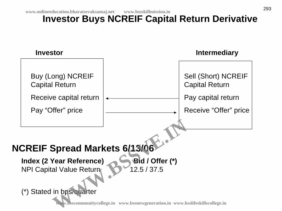
Investor Buys NCREIF Capital Return Derivative
Buy (Long) NCREIF Capital Return
Receive capital return
Pay “Offer” price
Investor Intermediary
Sell (Short) NCREIF Capital Return
Pay capital return
Receive “Offer” price
Index (2 Year Reference) Bid / Offer (*)NPI Capital Value Return 12.5 / 37.5
NCREIF Spread Markets 6/13/06
(*) Stated in bps/quarterwww.bsscommunitycollege.in www.bssnewgeneration.in www.bsslifeskillscollege.in
293www.onlineeducation.bharatsevaksamaj.net www.bssskillmission.in
WWW.BSSVE.IN

Payoff if long capital return
Year Quarter Capital Return Fixed Leg Difference2006 3 2.00% 0.38% 1.63%2006 4 3.03% 0.38% 2.66%
Long position would have received 1.63% in the 3rd quarter of 2006 and 2.66% in the fourth quarter. But what about next 6 quarters?
www.bsscommunitycollege.in www.bssnewgeneration.in www.bsslifeskillscollege.in
294www.onlineeducation.bharatsevaksamaj.net www.bssskillmission.in
WWW.BSSVE.IN

Investor Sells NCREIF Capital Return Derivative
Sell (Short) NCREIF Capital Return
Pay capital return
Receive “Bid” price
Investor CSFB
Buy (Long) NCREIF Capital Return
Receive capital return
Pay “Bid” price
Index (2 Year Reference) Bid / Offer (*)NPI Capital Value Return 12.5 / 37.5
NCREIF Spread Markets 6/13/06
(*) Stated in bps/quarter
Intermediary
www.bsscommunitycollege.in www.bssnewgeneration.in www.bsslifeskillscollege.in
295www.onlineeducation.bharatsevaksamaj.net www.bssskillmission.in
WWW.BSSVE.IN

Short position
Short position would have paid 1.88% in the 3rd quarter of 2006 and 2.91% in the fourth quarter. Perhaps next 6 quarters will be better!
Year Quarter Capital Return Fixed Leg Difference2006 3 2.00% 0.13% -1.88%2006 4 3.03% 0.13% -2.91%
www.bsscommunitycollege.in www.bssnewgeneration.in www.bsslifeskillscollege.in
296www.onlineeducation.bharatsevaksamaj.net www.bssskillmission.in
WWW.BSSVE.IN

Intermediary is Long and Short NCREIF Capital Return Derivative – nets bid ask spread.
Long and Short NCREIF Capital Return
Net “Bid Ask Spread”:(37.5 – 12.5 = 25)
Investor 2CSFB
Sell (Short) NCREIF Capital Return
Pay capital return
Pay “Bid” price (12.5)
Buy (Long) NCREIF Capital Return
Receive capital return
Pay “Ask” price (37.5)
Investor 1 Intermediary
www.bsscommunitycollege.in www.bssnewgeneration.in www.bsslifeskillscollege.in
297www.onlineeducation.bharatsevaksamaj.net www.bssskillmission.in
WWW.BSSVE.IN

Investor Swaps Office for Retail
Sell (short) Office
Buy (long) Retail
Pay Office return
Receive Retail price
Pay “Bid” price
Investor CSFB
Buy (Long) Office Return
Sell (Short) Retail Return
Receive Office Return
Pay Retail Return
Receive “Bid” price
(*) Stated in bps/quarter
NCREIF Spread Markets 6/13/06Index (2 Year Reference) Bid / Offer (*)Office vs. Retail Total Return 35.0 / 70.0
Bid is for intermediary to buy office and sell retail.
Intermediary
Property Type Swaps
www.bsscommunitycollege.in www.bssnewgeneration.in www.bsslifeskillscollege.in
298www.onlineeducation.bharatsevaksamaj.net www.bssskillmission.in
WWW.BSSVE.IN

Investor Purchases NCREIF Total Return (Income and Capital Return)
Buy (long) NCREIF Total Return
Receive total return
Pay Libor
Pay “Offer” price
Investor CSFB
Sell (Short) Total Return
Pay Total Return
Receive Libor
Receive “Offer” price
NCREIF Spread Markets 6/13/06Index (2 Year Reference) Bid / Offer (**)NPI Total Return L + 250 / L + 375
(**) Stated in bps/year ; L is 3-month Libor
Intermediary
www.bsscommunitycollege.in www.bssnewgeneration.in www.bsslifeskillscollege.in
299www.onlineeducation.bharatsevaksamaj.net www.bssskillmission.in
WWW.BSSVE.IN

Use of long position in R.E. Index Swap to Achieve Effect of Target R.E. Allocation in Portfolio Risk & Return Performance: A 2-step process…
Capital flows in first instance to debt market, helping keep interest rates low.
(1) Original Portfolio:Equity: $1.5 B ( 50%)Fixed Inc: $1.5 B ( 50%)R.E.: $ 0 B ( 0%)Total: $3.0 B (100%)
(2) Sell Stocks, Buy Riskless Bonds:Equity: Δ – $500 M $1.0 B ( 33.3%)Fixed Inc: Δ + $500 M $2.0 B ( 66.7%)R.E.: Δ 0 $ 0 B ( 0.0%)Total: Δ 0 $3.0 B (100%)
Step 2: Earmark $1.0 Billion of Fixed Income Allocation to Riskless Bonds to Cover Fixed Spread Obligation in R.E. Index Swap.
No cash changes hands up front, but effect on portfolio risk & return is as if:
Using Derivatives to Achieve Portfolio Target Real Estate Allocation
(3) Long in Swap, Cover with Bonds New Portfolio:Equity: $1.0 B, Δ 0 $1.0 B ( 33.3%)Fixed Inc.: $2.0 B, Δ – $1.0 B $1.0 B ( 33.3%)R.E.: $ 0 B, Δ + $1.0 B $1.0 B ( 33.3%)Total: $3.0 B, Δ 0 $3.0 B (100%)
www.bsscommunitycollege.in www.bssnewgeneration.in www.bsslifeskillscollege.in
300www.onlineeducation.bharatsevaksamaj.net www.bssskillmission.in
WWW.BSSVE.IN

Two Major Types of R.E. Indexes• Appraisal-based (e.g., NCREIF)
• Track a particular sub-population in which ALL properties are appraised EVERY period (or almost)
• Use the avg appraised value to represent Vt in the index return At ≈ Vt : rt ≈ (At – At-1)/At-1 .
• Transaction Price-based (e.g., “repeat-sales”)• Base index directly and purely on contemporaneous
transaction prices of the sample of properties that happens to sell each period
• Use statistics/econometrics to estimate population return (price change) each period.
Real estate derivatives depend on good indexes of real estate market returns, to serve as the basis of the derivatives…
www.bsscommunitycollege.in www.bssnewgeneration.in www.bsslifeskillscollege.in
301www.onlineeducation.bharatsevaksamaj.net www.bssskillmission.in
WWW.BSSVE.IN

NCREIF Index vs Transactions-Based Capital Value Index: 1984-2006, Quarterly
50
100
150
200
250
1984
1
1985
1
1986
1
1987
1
1988
1
1989
1
1990
1
1991
1
1992
1
1993
1
1994
1
1995
1
1996
1
1997
1
1998
1
1999
1
2000
1
2001
1
2002
1
2003
1
2004
1
2005
1
2006
1
Source: Fisher, Geltner & Pollakow ski (2006).
NPI Appreciation (EWCF) Transactions-Based
Appraisal-based index tends to smooth and lag the market.
Transaction-based index needs to guard against excessive noise.
www.bsscommunitycollege.in www.bssnewgeneration.in www.bsslifeskillscollege.in
302www.onlineeducation.bharatsevaksamaj.net www.bssskillmission.in
WWW.BSSVE.IN

NCREIF Index vs Transactions-Based Capital Value Index: 1984-2006, Quarterly
50
100
150
200
250
1984
1
1985
1
1986
1
1987
1
1988
1
1989
1
1990
1
1991
1
1992
1
1993
1
1994
1
1995
1
1996
1
1997
1
1998
1
1999
1
2000
1
2001
1
2002
1
2003
1
2004
1
2005
1
2006
1
Source: Fisher, Geltner & Pollakow ski (2006).
NPI Appreciation (EWCF) Transactions-Based
1990-91Recession
2001-02Recession
1998-99Fin Crisis,REIT Bust1986
Tax Reform
'87 Stk Mkt Crash
1992-93Kimco Taubman
IPOs
1997REITBoom
2005-6R.E.
Boom
Hedonic transactions-based index with noise filter:Most volatility is probably real…
www.bsscommunitycollege.in www.bssnewgeneration.in www.bsslifeskillscollege.in
303www.onlineeducation.bharatsevaksamaj.net www.bssskillmission.in
WWW.BSSVE.IN
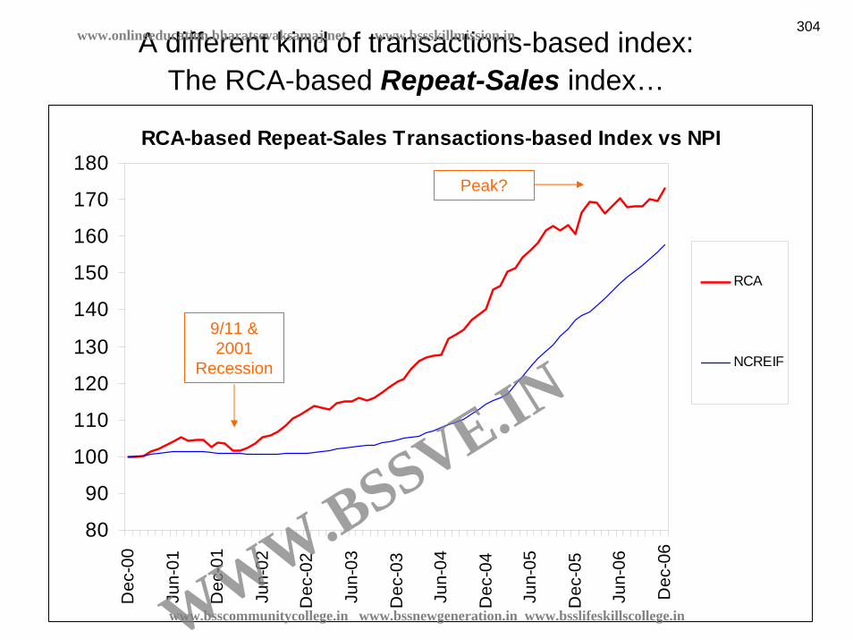
A different kind of transactions-based index:The RCA-based Repeat-Sales index…
RCA-based Repeat-Sales Transactions-based Index vs NPI
80
90
100
110
120
130
140
150
160
170
180
Dec
-00
Jun
-01
Dec
-01
Jun
-02
Dec
-02
Jun
-03
Dec
-03
Jun
-04
Dec
-04
Jun
-05
Dec
-05
Jun
-06
Dec
-06
RCA
NCREIF
Peak?
9/11 & 2001
Recession
www.bsscommunitycollege.in www.bssnewgeneration.in www.bsslifeskillscollege.in
304www.onlineeducation.bharatsevaksamaj.net www.bssskillmission.in
WWW.BSSVE.IN

R.E. Index Swaps Trading GamePut yourself in the shoes of one of two potential trading parties, in an imaginary scenario…
NewBalance Pension Fund currently has total assets of $300 million: $150M in stocks, $150M in bonds…• CIO wants more diversification (less volatility), & is worried about near-term future outlook for stock & bond returns.• Objective: Diversify quickly into real estate to obtain a balanced mixed-asset exposure across all 3 asset classes.
HedgeHog Asset Mgt.: Fund with specialized real estate expertise, a $100M all-real-estate fund that consistently earns positive alpha (beats RE index): Advertises alpha & protection of principal...• CIO worried about near-term direction of RE mkts.• Objective: Hedge RE mkt exposure, harvest alpha.
www.bsscommunitycollege.in www.bssnewgeneration.in www.bsslifeskillscollege.in
305www.onlineeducation.bharatsevaksamaj.net www.bssskillmission.in
WWW.BSSVE.IN
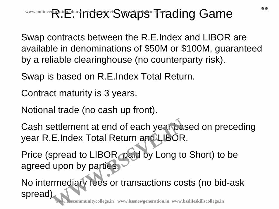
R.E. Index Swaps Trading Game
Swap contracts between the R.E.Index and LIBOR are available in denominations of $50M or $100M, guaranteed by a reliable clearinghouse (no counterparty risk).
Swap is based on R.E.Index Total Return.
Contract maturity is 3 years.
Notional trade (no cash up front).
Cash settlement at end of each year based on preceding year R.E.Index Total Return and LIBOR.
Price (spread to LIBOR, paid by Long to Short) to be agreed upon by parties.
No intermediary fees or transactions costs (no bid-ask spread).
www.bsscommunitycollege.in www.bssnewgeneration.in www.bsslifeskillscollege.in
306www.onlineeducation.bharatsevaksamaj.net www.bssskillmission.in
WWW.BSSVE.IN

R.E. Index Swaps Trading GameYour job:1. Decide whether you want to enter the Swap
market, and on which side (long or short), and for how much ($50 or $100M contract).
2. Think about what price (spread to LIBOR) you think is fair, and/or what price you would agree to (for how much notional). (10 min for 1 & 2)
3. Negotiate a swap price and amount with one or more counterparties. (10 min)
4. Identify (and we’ll assume you’ll carry out) any other related covering or structuring investment transactions. (Just make a note: no time reqd)
www.bsscommunitycollege.in www.bssnewgeneration.in www.bsslifeskillscollege.in
307www.onlineeducation.bharatsevaksamaj.net www.bssskillmission.in
WWW.BSSVE.IN

R.E. Index Swaps Trading GameOur job: We’ll create the future ! . . .We’ll roll the clock forward one year at a time, and
we’ll see how each of you has done (calculate net cash flow)
After each year, and in total (after all 3 years, net):Metrics: Compare:Under Status Quo As Negotiated(no swap trade): (with swap trade):
Periodic returns Periodic returnsOverall avg return* Overall avg return*Volatility Volatility
*Assume all cash reinvested per status quo: Time-wtd GMean ≈ IRR.
www.bsscommunitycollege.in www.bssnewgeneration.in www.bsslifeskillscollege.in
308www.onlineeducation.bharatsevaksamaj.net www.bssskillmission.in
WWW.BSSVE.IN

R.E. Index Swaps Trading GamePossibly relevant (or not?) background info:Current time is end of Year 0.Recent past history of Stock, Bond, & R.E. markets (as tracked by relevant indexes) Total Returns:Year: Stocks: Bonds: R.E.: LIBOR:-2 15% 5% 10% 3%-1 -15% 0% 20% 3%0 10% -3% 10% 3%Current LIBOR rates for 1, 2, & 3-yr maturity = 3%.Stock, Bond, & RE mkts (indexes) reflect equilibrium prices in those markets.No transactions costs for any trades in the stock, bond, or LIBOR markets.Hedge Hog will continue to earn 2%/yr positive alpha.
www.bsscommunitycollege.in www.bssnewgeneration.in www.bsslifeskillscollege.in
309www.onlineeducation.bharatsevaksamaj.net www.bssskillmission.in
WWW.BSSVE.IN

Asset Markets Outcomes & NewBalance Results:Future Ex Post Returns: NewBalance Returns:
End of Yr: Stk Retn Bnd Retn RE Retn LIBOR HHAM alpha Yr: w Swap wout Swap Differ:1 1 0.00% 0.00% 0.00%2 2 0.00% 0.00% 0.00%3 3 0.00% 0.00% 0.00%
GMean: 0.00% 0.00% 0.00% GMean: 0.00% 0.00% 0.00%Volatility: #DIV/0! #DIV/0! #DIV/0! Volatility: 0.00% 0.00% 0.00%
Notional Amt of Swap: WITH SWAPPrice (Spread to LIBOR):
NewBalance Assets: Change in Value: Returns:End of Yr: TotAssets Stocks Bonds LIBORcover TotAssets Stocks Bonds LIBORcover Swap
0 $300.00 $150.00 $150.00 $0.001 $300.00 $150.00 $150.00 $0.00 $0.00 $0.00 $0.00 $0.00 $0.00 0.00%2 $300.00 $150.00 $150.00 $0.00 $0.00 $0.00 $0.00 $0.00 $0.00 0.00%3 $300.00 $150.00 $150.00 $0.00 $0.00 $0.00 $0.00 $0.00 $0.00 0.00%
GMean Return: 0.00% AMean: 0.00%Volatility: 0.00%
Notional Amt of Swap: $0 WITHOUT SWAPPrice (Spread to LIBOR): 0.00%
NewBalance Assets: Change in Value: Returns:End of Yr: TotAssets Stocks Bonds LIBORcover TotAssets Stocks Bonds LIBORcover Swap
0 $300.00 $150.00 $150.00 $0.001 $300.00 $150.00 $150.00 $0.00 $0.00 $0.00 $0.00 $0.00 $0.00 0.00%2 $300.00 $150.00 $150.00 $0.00 $0.00 $0.00 $0.00 $0.00 $0.00 0.00%3 $300.00 $150.00 $150.00 $0.00 $0.00 $0.00 $0.00 $0.00 $0.00 0.00%
GMean Return: 0.00% AMean: 0.00%Volatility: 0.00%
R.E. Index Swaps Trading GameNewBalance Results: Fill in the blanks using Excel . . .
www.bsscommunitycollege.in www.bssnewgeneration.in www.bsslifeskillscollege.in
310www.onlineeducation.bharatsevaksamaj.net www.bssskillmission.in
WWW.BSSVE.IN
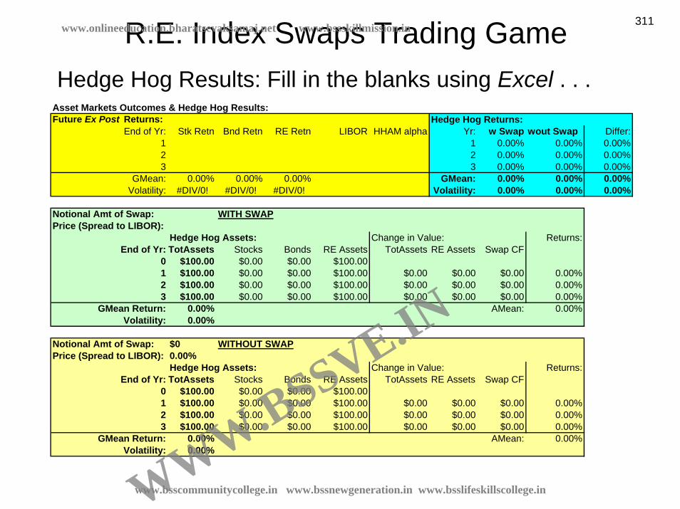
R.E. Index Swaps Trading GameHedge Hog Results: Fill in the blanks using Excel . . .
Asset Markets Outcomes & Hedge Hog Results:Future Ex Post Returns: Hedge Hog Returns:
End of Yr: Stk Retn Bnd Retn RE Retn LIBOR HHAM alpha Yr: w Swap wout Swap Differ:1 1 0.00% 0.00% 0.00%2 2 0.00% 0.00% 0.00%3 3 0.00% 0.00% 0.00%
GMean: 0.00% 0.00% 0.00% GMean: 0.00% 0.00% 0.00%Volatility: #DIV/0! #DIV/0! #DIV/0! Volatility: 0.00% 0.00% 0.00%
Notional Amt of Swap: WITH SWAPPrice (Spread to LIBOR):
Hedge Hog Assets: Change in Value: Returns:End of Yr: TotAssets Stocks Bonds RE Assets TotAssets RE Assets Swap CF
0 $100.00 $0.00 $0.00 $100.001 $100.00 $0.00 $0.00 $100.00 $0.00 $0.00 $0.00 0.00%2 $100.00 $0.00 $0.00 $100.00 $0.00 $0.00 $0.00 0.00%3 $100.00 $0.00 $0.00 $100.00 $0.00 $0.00 $0.00 0.00%
GMean Return: 0.00% AMean: 0.00%Volatility: 0.00%
Notional Amt of Swap: $0 WITHOUT SWAPPrice (Spread to LIBOR): 0.00%
Hedge Hog Assets: Change in Value: Returns:End of Yr: TotAssets Stocks Bonds RE Assets TotAssets RE Assets Swap CF
0 $100.00 $0.00 $0.00 $100.001 $100.00 $0.00 $0.00 $100.00 $0.00 $0.00 $0.00 0.00%2 $100.00 $0.00 $0.00 $100.00 $0.00 $0.00 $0.00 0.00%3 $100.00 $0.00 $0.00 $100.00 $0.00 $0.00 $0.00 0.00%
GMean Return: 0.00% AMean: 0.00%Volatility: 0.00%
www.bsscommunitycollege.in www.bssnewgeneration.in www.bsslifeskillscollege.in
311www.onlineeducation.bharatsevaksamaj.net www.bssskillmission.in
WWW.BSSVE.IN

R.E. Index Swaps Trading GameExample game outcome…Suppose future returns turn out ex post as follows:Year: Stocks: Bonds: R.E.: LIBOR:1 8% 4% -5% 3%2 -17% -11% 2% 3%3 -2% -1% -4% 3%
And Hedge Hog makes 2% positive alpha each year.Swap traded: NewBalance long, Hedge Hog short:$100M @ LIBOR (no spread) – which is the equilibrium price (assuming indexes were in equilibrium).Then 3-yr results compared to status quo (no swap):
• NewBalance: Mean return up 47bps, Volatility down 452bps.• Hedge Hog: Mean return up 515bps, Volatility down 342bps: earns pos retns even tho RE is down.
www.bsscommunitycollege.in www.bssnewgeneration.in www.bsslifeskillscollege.in
312www.onlineeducation.bharatsevaksamaj.net www.bssskillmission.in
WWW.BSSVE.IN

R.E. Index Swaps Trading GameNewBalance Example Results (a given future “history”,
$100M notional trade at LIBOR flat):Asset Markets Outcomes & NewBalance Results:Future Ex Post Returns: NewBalance Returns:
End of Yr: Stk Retn Bnd Retn RE Retn LIBOR HHAM alpha Yr: w Swap wout Swap Differ:1 8.00% 4.00% -5.00% 3.00% 2.00% 1 2.33% 6.00% -3.67%2 -17.00% -11.00% 2.00% 3.00% 2.00% 2 -8.79% -14.00% 5.21%3 -2.00% -1.00% -4.00% 3.00% 2.00% 3 -2.39% -1.50% -0.89%
GMean: -4.23% -2.87% -2.38% GMean: -3.06% -3.53% 0.47%Volatility: 12.58% 7.64% 3.79% Volatility: 5.58% 10.10% -4.52%
Notional Amt of Swap: $100 WITH SWAPPrice (Spread to LIBOR): 0.00%
NewBalance Assets: Change in Value: Returns:End of Yr: TotAssets Stocks Bonds LIBORcover TotAssets Stocks Bonds LIBORcover Swap
0 $300.00 $100.00 $100.00 $100.001 $307.00 $103.50 $103.50 $100.00 $7.00 $8.00 $4.00 $3.00 -$8.00 2.33%2 $280.02 $90.01 $90.01 $100.00 -$26.98 -$17.60 -$11.39 $3.00 -$1.00 -8.79%3 $273.32 $86.66 $86.66 $100.00 -$6.70 -$1.80 -$0.90 $3.00 -$7.00 -2.39%
GMean Return: -3.06% AMean: -2.95%Volatility: 5.58%
Notional Amt of Swap: $0 WITHOUT SWAPPrice (Spread to LIBOR): 0.00%
NewBalance Assets: Change in Value: Returns:End of Yr: TotAssets Stocks Bonds LIBORcover TotAssets Stocks Bonds LIBORcover Swap
0 $300.00 $150.00 $150.00 $0.001 $318.00 $159.00 $159.00 $0.00 $18.00 $12.00 $6.00 $0.00 $0.00 6.00%2 $273.48 $136.74 $136.74 $0.00 -$44.52 -$27.03 -$17.49 $0.00 $0.00 -14.00%3 $269.38 $134.69 $134.69 $0.00 -$4.10 -$2.73 -$1.37 $0.00 $0.00 -1.50%
GMean Return: -3.53% AMean: -3.17%Volatility: 10.10%
www.bsscommunitycollege.in www.bssnewgeneration.in www.bsslifeskillscollege.in
313www.onlineeducation.bharatsevaksamaj.net www.bssskillmission.in
WWW.BSSVE.IN
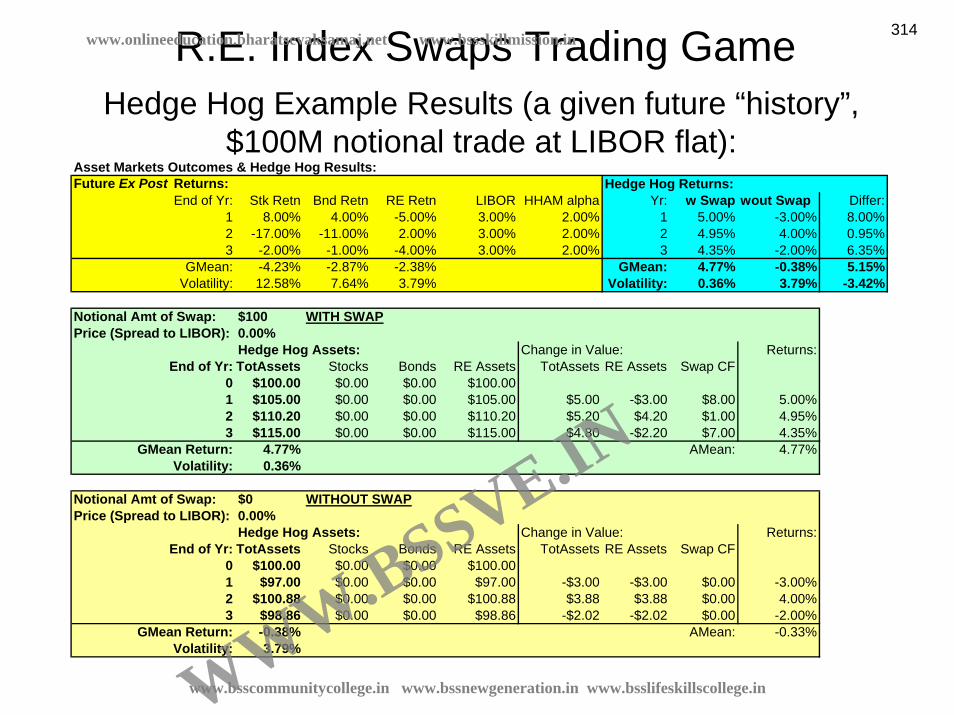
R.E. Index Swaps Trading GameHedge Hog Example Results (a given future “history”,
$100M notional trade at LIBOR flat):Asset Markets Outcomes & Hedge Hog Results:Future Ex Post Returns: Hedge Hog Returns:
End of Yr: Stk Retn Bnd Retn RE Retn LIBOR HHAM alpha Yr: w Swap wout Swap Differ:1 8.00% 4.00% -5.00% 3.00% 2.00% 1 5.00% -3.00% 8.00%2 -17.00% -11.00% 2.00% 3.00% 2.00% 2 4.95% 4.00% 0.95%3 -2.00% -1.00% -4.00% 3.00% 2.00% 3 4.35% -2.00% 6.35%
GMean: -4.23% -2.87% -2.38% GMean: 4.77% -0.38% 5.15%Volatility: 12.58% 7.64% 3.79% Volatility: 0.36% 3.79% -3.42%
Notional Amt of Swap: $100 WITH SWAPPrice (Spread to LIBOR): 0.00%
Hedge Hog Assets: Change in Value: Returns:End of Yr: TotAssets Stocks Bonds RE Assets TotAssets RE Assets Swap CF
0 $100.00 $0.00 $0.00 $100.001 $105.00 $0.00 $0.00 $105.00 $5.00 -$3.00 $8.00 5.00%2 $110.20 $0.00 $0.00 $110.20 $5.20 $4.20 $1.00 4.95%3 $115.00 $0.00 $0.00 $115.00 $4.80 -$2.20 $7.00 4.35%
GMean Return: 4.77% AMean: 4.77%Volatility: 0.36%
Notional Amt of Swap: $0 WITHOUT SWAPPrice (Spread to LIBOR): 0.00%
Hedge Hog Assets: Change in Value: Returns:End of Yr: TotAssets Stocks Bonds RE Assets TotAssets RE Assets Swap CF
0 $100.00 $0.00 $0.00 $100.001 $97.00 $0.00 $0.00 $97.00 -$3.00 -$3.00 $0.00 -3.00%2 $100.88 $0.00 $0.00 $100.88 $3.88 $3.88 $0.00 4.00%3 $98.86 $0.00 $0.00 $98.86 -$2.02 -$2.02 $0.00 -2.00%
GMean Return: -0.38% AMean: -0.33%Volatility: 3.79%
www.bsscommunitycollege.in www.bssnewgeneration.in www.bsslifeskillscollege.in
314www.onlineeducation.bharatsevaksamaj.net www.bssskillmission.in
WWW.BSSVE.IN

R.E. Index Swaps Trading GamePrevious example outcome is just illustrious, but:• Swaps do enable investors to quickly diversify into real estate (effectively adding R.E. into the portfolio) at low transaction cost and with diversified R.E. holdings (index); and• This does tend to reduce overall mixed-asset portfolio volatility (or higher returns at the same volatility using leverage), by reducing overexposure to stocks & bonds.• Swaps do enable real estate investors to hedge against R.E. market downturns, protecting principal & enabling harvesting of positive “alpha”(generated by R.E. experts).www.bsscommunitycollege.in www.bssnewgeneration.in www.bsslifeskillscollege.in
315www.onlineeducation.bharatsevaksamaj.net www.bssskillmission.in
WWW.BSSVE.IN

One Lincoln Street (B)
Timing, luck, and a little bit of guts. That’s how John Hynes summarized the recipe for success for the One Lincoln Street development. But Linda Douglass, Senior Acquisition Officer for Atlantic-Pacific Property Corp., wasn’t buying John’s latest attempt at humility. Linda had bought more than a billion dollars of property over the past five years and knew all too well the amount of negotiating, positioning, persuasion and determination needed to develop a spec building in Boston.
As coffee was being served and their lunch was coming to an end, it was clear that Linda wanted to know more about the construction and financial status of One Lincoln Street, and to pick up on John’s seemingly off-hand comment regarding how Gale & Wentworth might best proceed to monetize the substantial investment value it had created during the development and lease-up phases. Linda had known John for over 15 years dating back to when she was an analyst for a private real estate fund that acquired multi-family apartments. Now at Atlantic-Pacific, this was the first time she had the sense there might be a real transaction for her and John to explore.
Background
In mid-1999, John Hynes identified − and then secured − a million square foot office development opportunity adjacent to South Station in Boston. The project, known as One Lincoln Street, had been kicking around for years but could never find a way to get off the ground. That is, not until the office market came storming back and John Hynes and his partners at Morgan Stanley stepped into the breach and committed enough capital to complete the required site assemblage and perfect the entitlements necessary to proceed to construction. Beyond that, all that was needed was another $300 million and a tenant or two.
As it turned out, the capital was delivered first courtesy of Midwest State Teachers Retirement System (“STRS”). They, too, believed in the long-term vibrancy of the Boston office market and committed over $150 million of equity to commence construction and secure required construction financing. And to everyone’s surprise, John (with a little help from the overheated Boston office market) actually convinced STRS to flex their investment policies a wee bit and proceed to construction on a speculative basis.
That’s when the unexpected occurred.
This case was prepared by W. Tod McGrath for the purpose of class discussion. The case describes a hypothetical situation and is not intended to illustrate either effective of ineffective handling of a fiduciary situation. Revised February 2007.
www.bsscommunitycollege.in www.bssnewgeneration.in www.bsslifeskillscollege.in
316www.onlineeducation.bharatsevaksamaj.net www.bssskillmission.in
WWW.BSSVE.IN

So much of John’s time and energy had been spent negotiating the terms and conditions of the site acquisition, construction loan documentation, and joint-venture structure that he hadn’t even begun to seriously engage the marketing effort for the project. Day-in and day-out his focus was on finalizing the papering of the deal so he could break ground and prove to the marketplace that he had a real project. He never expected to have a letter of intent signed for any space in the building before the heavy site work began. And he certainly never expected to receive a call from Commonwealth Avenue Custody Corporation asking if he could quickly respond to an RFP for 700,000 square feet of space before the construction drawings were even submitted to the city for review.
But what was really unexpected was the actual signing of a lease with Commonwealth Avenue before the first yard of concrete was poured. And not for 700,000 square feet; but for each and every of the 1,025,000 rentable square feet in the building. Along with the parking garage. For 20 years. With rent bumps.
Now that was unexpected.1
Venture Dynamics
You’d think a 20-year lease with AA- rated credit would simplify things. Not necessarily. As John motioned to the waiter for the check, he mentioned to Linda that he had to catch a shuttle to New York for a late afternoon meeting with Morgan Stanley. Despite the project being on schedule, slightly under budget (due to a drop in short-term interest rates), and ready for certificates of occupancy on the first 20 floors, there was a certain restlessness brewing within the venture. MSGW III, the fund that supplied the remaining 10% of the initial equity not otherwise committed by STRS, was strategically reviewing its asset allocations and debating the wisdom of monetizing or selling its equity position in the project. After all, MSGW III was an opportunity fund that advertised a 5-year expected life, and had had a substantial amount of capital committed to One Lincoln Street without any return for over 3 years.
While thrilled with the overall outcome of the Commonwealth Avenue lease, the space and capital markets had changed rather dramatically since the initial equity funding. In the space markets, Class-A vacancy rates (including sublease space) increased from under 4% in 1999 to approximately 5%, 10% and 15% in 2000, 2001, and 2002, respectively. Current (mid 2003) vacancy rates approached 16% (see Exhibit 1). Asking rents for Class-A space had decreased about 25% from about $65 per rentable square foot in 2000 to $50 or less in mid 2003, and most market watchers expected continued decreases throughout the remainder of the year. Current effective rents (incorporating free rent concessions, above-standard tenant improvements, etc.) were now at least 10% lower than asking rents.
In the capital markets, interest rates on both long and short term debt instruments had also decreased significantly. Yields on 10-year Treasury securities had decreased from about 6.50% in early 2000 to about 3.75% in mid 2003. Yields on 15 and 20-year Treasury
1 The unusually prolonged closing festivities, however, were not.
2
www.bsscommunitycollege.in www.bssnewgeneration.in www.bsslifeskillscollege.in
317www.onlineeducation.bharatsevaksamaj.net www.bssskillmission.in
WWW.BSSVE.IN

securities were currently about 4.00% and 4.25%, respectively. The combination of these trends – weakening space market fundamentals and historically low interest rates – made the Morgan Stanley crowd fairly serious about the idea of harvesting profits.
And then there was STRS. As part of its ongoing asset management discipline, STRS was similarly reviewing its asset allocations, particularly within regions like greater Boston that had recently exhibited a high degree of both demand and rental rate volatility. Due to its relatively unique leasing profile, STRS was quite comfortable with its investment in One Lincoln Street; so much so that members of the asset management staff routinely joked about transferring their joint-venture interest in One Lincoln Street to the fixed income group in exchange for a few more days of paid vacation.
Some others within the asset management group, however, were thinking a bit more seriously. Included within the venture documentation were heavily negotiated provisions relating to mechanisms by which both STRS and MSGW could either acquire each other’s interest in the venture or divest their existing interests. Indeed, one senior asset manager was openly debating the long-term alignment of interest between STRS and MSGW, essentially asking why (now that the building is completed) is MSGW such a good long-term partner?
The leasing profile of One Lincoln Street made it exactly the type of asset STRS sought to acquire: one that generated safe, long-term cash flows with predictable built-in growth and little or no future capital expenditures. And STRS was having more than a bit of trouble finding similar type assets, particularly ones that were fairly priced. It was because STRS believed that the negotiated acquisition mechanisms within the venture would deliver fair prices to either party, that some serious discussions had begun regarding triggering the operation of the venture’s Buy/Sell provisions to acquire MSGW’s interest.
And, yes, Morgan Stanley (and now Gale & Wentworth) had gotten wind of it.
The Buy/Sell Provisions
They worked like this:
Any time after shell completion, either STRS or MSGW could submit an offer to purchase the other party’s entire equity interest in the development by delivering to the other party a Buy/Sell Offering Notice that included a “Specified Valuation Amount” which the offering party would be willing to pay in cash for one hundred percent (100%) fee ownership of the development;
The non-offering party would then have 45 days to notify the offering party whether or not it elected to
� sell (as “Seller”) its entire equity interest in the development to the offering party for a price equal to the amount the non-offering party would have received had the development been sold for the Specified Valuation Amount, or
3
www.bsscommunitycollege.in www.bssnewgeneration.in www.bsslifeskillscollege.in
318www.onlineeducation.bharatsevaksamaj.net www.bssskillmission.in
WWW.BSSVE.IN

� acquire (as “Purchaser”) the entire equity interest in the development of the offering party for a price equal to the amount the offering party would have received had the development been sold for the Specified Valuation Amount;
If the non-offering party failed to notify the offering party of its election prior to the 45-day Buy/Sell election period, then the offering party could acquire as Purchaser the entire equity interest of the non-offering party;
At the time of either party’s election to purchase, the Purchaser would be required to make a non-refundable deposit to the Seller equal to five percent (5%) of the amount the Seller would otherwise receive;
If the Purchaser failed to perform, in breach of its purchase obligation, then the Purchaser would (i) forfeit its five percent (5%) deposit, (ii) be responsible for all closing costs actually incurred (including, without limitation, escrow costs and transfer taxes), and (iii) lose all future rights to trigger the Buy/Sell provisions thereafter; and
As a result of the breach of the Purchaser’s obligations, the Seller would have the option, within 30 days of default by the Purchaser, of substituting itself as Purchaser and thereupon have the right to Purchase the other party’s entire equity interest in the development for eighty-five percent (85%) of the amount that the other party would have otherwise received had the development been sold for the Specified Valuation Amount.
Trouble in Paradise?
On the shuttle to Manhattan, John couldn’t help but think of how much he wanted to preserve an ownership interest in the asset he had worked so hard to create. From his perspective, he was in the development business for the long haul – not the quick flip. He understood only too well that a development deal like One Lincoln Street happens once in a career – and only if your timing’s damn good and you’re damn lucky and you’ve got a lot of guts. The guys at Morgan Stanley didn’t understand that; or even if they did, they couldn’t care less about his personal business philosophy. He knew the conversation would be about “harvesting” and “rebalancing” and “posting numbers”. And he knew he wasn’t going to be happy with a decision to sell out to STRS.
Unfortunately, the meeting went pretty much as he predicted. Morgan Stanley reiterated their understanding that STRS was preparing a Buy/Sell Offering Notice that contained the required Specified Valuation Amount, and that such Specified Valuation Amount was being established through an independent MAI appraisal process (see Exhibit 2 for recent building sales information). In addition, Morgan Stanley presented all of their high-brow reasons for why they needed to cash out and how they would try to position STRS to get the highest possible valuation for One Lincoln Street. But despite all the pinstriped bravado, one thing was clear from the meeting: if MSGW didn’t like the Specified Valuation Amount offered to them by STRS, they weren’t in a very good
4
www.bsscommunitycollege.in www.bssnewgeneration.in www.bsslifeskillscollege.in
319www.onlineeducation.bharatsevaksamaj.net www.bssskillmission.in
WWW.BSSVE.IN

position to come up with over a half billion dollars in 45 days to exercise their option to buy out STRS’ interest. They didn’t have a plan for that; they didn’t even have a plan for a plan. At least not until John Hynes put a call into Linda Douglass from the shuttle back to Boston to set up a meeting at his office for early the following morning.
Plan B
Linda arrived at John’s office at 8:00 am. She was more than a little curious as to why he wanted to meet so quickly. Before she even had the time to put milk in her coffee, John had already launched into a discourse on the status of the One Lincoln Street development and the impending ownership issues within the venture. Then John pointedly asked Linda if Atlantic-Pacific had the financial capacity to make a credible purchase offer for the property and if she was willing to conditionally explore such an acquisition.
She responded “Yes. Yes. And what exactly do you mean by conditionally?”
John explained “conditionally”: he was willing to give Linda an exclusive opportunity to submit an informal purchase offer to acquire a majority ownership interest in One Lincoln Street. Because he was presenting this acquisition opportunity exclusively to Atlantic-Pacific, he made it very clear to Linda that any informal purchase offer she submitted should be considered as “take-it-or-leave-it.” A formal purchase offer, if subsequently requested by MSGW and submitted by Atlantic-Pacific, would be in the same amount as the informal purchase offer and would, necessarily, be a “backstop” offer: that is,
it would be submitted to MSGW on the same basis that STRS would be required to submit its Specified Valuation Amount for the development (i.e., 100% fee ownership);
if such offer were greater than or equal to the Specified Valuation Amount submitted by STRS, MSGW would exercise its option to acquire STRS’ interest at a price equal to what STRS would otherwise receive if the development were sold for the Specified Valuation Amount;
the extent, if any, to which Atlantic-Pacific’s formal purchase offer exceeded the Specified Valuation Amount would be paid to MSGW in cash at closing; and
MSGW, or its assignee, could continue to own its current equity interest in the venture (or could elect to be partially cashed-out on a proportionate basis) and would continue to manage the development.
John was confident he could get Morgan Stanley to participate, at some level, within that framework. This was his opportunity to both harvest profits and stay in the deal. Simple enough, right?
Simple, but not that simple. Linda quickly pointed out to John that, as a vertically-integrated public real estate operating company, Atlantic-Pacific would never make a
5
www.bsscommunitycollege.in www.bssnewgeneration.in www.bsslifeskillscollege.in
320www.onlineeducation.bharatsevaksamaj.net www.bssskillmission.in
WWW.BSSVE.IN

substantial acquisition without controlling the management of the asset and being fairly compensated to do so. If John wanted a formal “backstop” purchase offer from Atlantic-Pacific, he could forget about retaining management or any portion of the management fee (of which an estimated 75% was net profit after allocated staff cost).
After a somewhat long and uncomfortable silence, John agreed to Linda’s rather firm position, but felt obligated to impose a few conditions of his own: namely, that (i) Atlantic-Pacific’s informal purchase offer was due within 10 calendar days, irrespective of when, or if, STRS ever delivered a Buy/Sell Offering Notice, (ii) as part of its formal purchase offer, Atlantic-Pacific would be required to indemnify MSGW against any and all financial loss or damage relating to Atlantic-Pacific’s failure to perform under such purchase offer, if such offer were formally accepted by MSGW, and (iii) based on Commonwealth Avenue’s credit, the absence of future landlord-funded capital expenditures, and the built-in rent steps throughout the initial 20-year lease term, he thought her offer price should start with a “7”. Linda wasn’t exactly sure how to evaluate John’s last condition, but she thought she understood the first two.
Linda left John’s office with an abstract of the 400+-page office lease with Commonwealth Avenue Custody Corporation and a promise to immediately receive mountains of due diligence materials on the legal and physical status of the building. As she walked back to her office, she thought about two things: one, the need to quickly marshal the resources of her acquisition team to commence the necessary due diligence; and two, the need to quickly review the lease abstract and attached projection of Property Before-Tax Cash Flow (see Exhibit 3). She’d done this many times before so she knew where to start and what to focus on.
The Lease and Lessee
The lease executed with Commonwealth Avenue Custody Corp. was a 20-year full service gross lease with tax and operating expense stops that ensured the lessor that virtually all increases in property taxes and operating expenses throughout the 20-year term of the lease would be fully reimbursed by Commonwealth Avenue as additional required rent. Under the terms of the lease, MSGW had provided a fixed tenant improvement allowance to Commonwealth Avenue (which had already been fully dispersed for construction of interior improvements), paid all required brokerage commissions, and agreed to limit its annual property management fees to about 0.9% of Effective Gross Income. The scheduled commencement date for the lease was only a few months away.
With over $6 trillion of assets under custody and more than three-quarters of a trillion dollars of assets under management, Commonwealth Avenue Custody Corporation was one of the leading servicers of financial assets in the world. Based in Boston, Commonwealth Avenue occupied well over a million square feet in the greater Boston area and was the sole tenant of One Lincoln Street. Commonwealth Avenue was publicly-traded and had an issuer credit rating of AA- by Standard & Poor’s, enabling it to borrow money in the long-term public bond markets at approximately 85 basis points over comparable-term U.S. Treasury securities.
6
www.bsscommunitycollege.in www.bssnewgeneration.in www.bsslifeskillscollege.in
321www.onlineeducation.bharatsevaksamaj.net www.bssskillmission.in
WWW.BSSVE.IN

Atlantic-Pacific Property Corporation
Linda started with Atlantic-Pacific shortly after it went public in the mid ‘90’s. As an acquisitions officer working for a publicly-traded REIT, Linda’s responsibility was to understand not only the micro-level dynamics of specific property markets, but to apply proven capital budgeting techniques and required financial accounting conventions to arrive at investment decisions that added value to Atlantic-Pacific’s growing franchise. An important part of Linda’s responsibility was to thoroughly understand the financial performance of Atlantic-Pacific and to integrate that understanding into value-enhancing capital investment decisions. Selected summary (historical) financial data for Atlantic-Pacific is presented in Exhibit 4.
In her frequent discussions with Atlantic-Pacific’s CFO, Linda had become aware of the CFO’s perspective and concerns relating to large deployments of investment capital. For any investment over $100 million, she’d been informed that the company would be required to issue both additional equity and unsecured debt. Atlantic-Pacific’s stock price had just recently regained the $44 share price it enjoyed about three years earlier. Over the past two years, Atlantic-Pacific had been very cautious about issuing new equity; however, after recently acquiring assets on its unsecured credit line, it found itself with a debt-to-total market capitalization ratio of approximately 50% − a threshold it didn’t really want to exceed. Any significant acquisition of property would most likely be financed with 50% equity (through a secondary public offering with an underwriters’ spread of 5%) and 50% unsecured debt which Atlantic-Pacific could issue at about 175 basis points over comparable-term treasuries, excluding financing fees and closing costs of about 25 basis points (see Exhibit 5).
Linda was also painfully aware of the fact that the company’s primary investment markets had softened rather significantly. As a result, the company’s “same portfolio” year-over-year cash-basis NOI growth rate had decreased from about 6% three years ago, to about 3% two years ago, to virtually no growth last year. Expectations for 2003 were for negative NOI growth (contraction) of about 1%.
According to the CFO, Atlantic-Pacific’s FFO per share, which had grown significantly over the past five years, was also now likely to plateau due to deteriorating property market fundamentals and the relatively small amount of existing secured mortgage debt available to be refinanced by the company at significantly lower rates. A few stock analysts were even reducing their estimates of Atlantic-Pacific’s FFO per share to slightly below the $4.00 level achieved in 2002. Based on increased market-based tenant improvement allowances and other structural characteristics of the company’s assets and liabilities, Atlantic-Pacific’s operating cash flow, as measured by its Funds Available for Distribution (FAD), was currently estimated at about 80% of its Funds From Operations (FFO), or about $3.20 per share. The analysts that estimated REIT Net Asset Values (NAV) were currently in the range of $39 to $42 for Atlantic-Pacific’s shares.
7
www.bsscommunitycollege.in www.bssnewgeneration.in www.bsslifeskillscollege.in
322www.onlineeducation.bharatsevaksamaj.net www.bssskillmission.in
WWW.BSSVE.IN

Screening
Based on everything that was happening at both the property and corporate levels, Linda knew the CFO was every bit as anxious to evaluate her preliminary bid as John Hynes was. Yet before taking the time to complete a comprehensive purchase offer analysis, she quickly put the cash-basis financial projection for the property (attached to the lease abstract given to her) through her first feasibility screen. The purpose of this screen was to determine if, at John Hynes’ purported $700 million minimum offer price, a hypothetical acquisition of a 100% fee ownership interest would generate a pro forma incremental cash surplus or deficiency to Atlantic-Pacific’s shareholders based on the assumed 50/50 debt/equity capitalization and current dividend payout levels (see Exhibit 6).
Her next financial feasibility screen was the financial reporting analog, or pro forma accretion/dilution to Funds From Operation (FFO)2 per share. For this acquisition, she would specifically assume that the only additional company-level general and administrative (G&A) expense would be (i) the building personnel costs included in the administrative cost line item of the property operating expense budget (Exhibit 3) and (ii) direct overhead costs equal to about 25% of the annual property management fee (implying the remaining 75% of the fee would be a new profit center to the company).
To prepare this accounting-based analysis, she knew she would need to adjust the Base Rental Revenue payable by Commonwealth Avenue to reflect the financial reporting conventions under generally accepted accounting principles (GAAP). These financial reporting conventions require that:
all contractual Base Rental Revenue (and any applicable free rent periods) be reported on a straight-line basis over the term of the lease, as opposed to the manner in which the specific annual contractual Base Rental payments would actually be received by Atlantic-Pacific, and
the present value3 of the “above-market” portion of the annual contractual Base Rents be amortized on a straight-line basis as a deduction in arriving at Earnings Before Interest, Taxes, Depreciation and Amortization (EBITDA). In this regard, Linda believed – and felt Atlantic-Pacific’s independent auditors may also believe – that, over the twenty-year term of the lease, the annual contractual Base Rents per square foot (reflecting the periodic rent bumps) were no less than about $15
2 For purposes of this financial feasibility screen, Linda knew she could quickly estimate the property’s contribution to the company’s existing annual FFO, as:
(i) the property’s annual Earnings Before Interest, Taxes, Depreciation and Amortization (under GAAP),
(ii) plus the “profit center” portion of the annual property management fee, (iii) less any incremental annual interest expense incurred in connection with acquiring the
property, (iv) less any amortization of applicable financing fees and costs.
3 Computed using an appropriate risk-adjusted discount rate reflecting the risk associated with collecting the contractual annual Base Rents.
8
www.bsscommunitycollege.in www.bssnewgeneration.in www.bsslifeskillscollege.in
323www.onlineeducation.bharatsevaksamaj.net www.bssskillmission.in
WWW.BSSVE.IN

per square foot per year above current market lease pricing for leases of comparable term.
Bid Preparation – The Final Frontier
Putting financial assumptions through preliminary feasibility screens is one thing; valuing a major real estate asset with conviction is quite another. Linda had a lot of information − and a lot of issues − to synthesize.
For example, she knew that an offer price of $700 million or more would imply a very low acquisition cap rate, even lower than the cap rates observed during the height of the market when the lease with Commonwealth Avenue was signed (cap rates on recent multi-tenant office building sales in Boston were in the 7.0% range). Linda also realized that while Commonwealth Avenue’s lease had contractual rent steps, it also had contractually limited rent growth. Then again, market rents in their core markets had been deteriorating and this asset might now represent an excellent long-term performance hedge for their portfolio. She then thought for a moment about some of the challenges associated with articulating those possibly conflicting arguments as part of her pricing recommendation, both to senior management and, ultimately, the REIT analyst community if Atlantic-Pacific ended up owning the building.
Linda knew she had to try to explicitly incorporate the somewhat unique characteristics of a 20-year lease and Commonwealth Avenue’s investment grade credit rating into the valuation of the asset on a stand-alone basis as well as an addition to Atlantic-Pacific’s existing portfolio cash flows. Linda understood that, from a default and loss perspective, the lease with Commonwealth Avenue was not quite the equivalent of a bond; however, she also knew that the uncertainty associated with collecting the annual rent from Commonwealth Avenue would be much less than that associated with collecting the annual rent from many of the tenants in other buildings owned by Atlantic-Pacific.
Senior management at Atlantic-Pacific believed that the legal structure of a lease generally imposed more obligations on a landlord than a bondholder in terms of being entitled to demand payment. That said, they had often argued that a leaseholder was more likely to get paid than a bondholder during the early stages of a tenant’s financial distress (in order for the tenant to keep the doors open and remain in business), but once a bankruptcy petition was filed by the tenant, the leaseholder (as an unsecured creditor) was likely to receive at least a third less in terms of percentage recovery than were bondholders (as secured creditors). This was primarily due to the tenant’s right to reject the lease as part of a confirmed reorganization plan under the federal bankruptcy code. Based on this reasoning, Linda figured that an additional 25 to 50 basis point premium over the yield on Commonwealth Avenue’s long term bonds was warranted when trying to determine the value of the Commonwealth Avenue lease.
There just seemed to be a lot of basic questions that were a little harder to answer on this deal than others she had worked on. For example:
How might Commonwealth Avenue’s Right-of-First Offer-on-Sale affect her valuation of the property? That right provides that:
9
www.bsscommunitycollege.in www.bssnewgeneration.in www.bsslifeskillscollege.in
324www.onlineeducation.bharatsevaksamaj.net www.bssskillmission.in
WWW.BSSVE.IN

� If the Landlord wishes to sell the property, it must first notify Commonwealth Avenue. Commonwealth Avenue then has 60 days to review the property and make an offer to purchase it.
� The Landlord is free to accept or reject Commonwealth Avenue’s offer.
� However, should the Landlord reject Commonwealth Avenue’s offer, it is free to sell the property to a third-party purchaser only if the sales price offered by such third-party purchaser is at least 2% greater than the price offered by Commonwealth Avenue.
What could the building be sold for in 20 years when the lease expired? The Commonwealth Avenue lease contains two 10-year renewal options (applicable to its entire premises); the first of which is at 95% of Fair Market Rent, the second at 100%. What’s the probability that Commonwealth Avenue would exercise its first renewal option?
If such renewal option(s) weren’t exercised, what would an owner have to reasonably expect to incur in terms of vacancy and tenant improvement and commission costs in connection with re-leasing the entire building?
Where would market rents and related operating and capital expenses be in 20 years? To Linda, twenty years seemed like a pretty long time; yet to her CFO, twenty weeks seemed like an eternity.
Based on Commonwealth Avenue’s twenty-year lease term, what effect, if any, could arranging debt financing for a term in excess of ten years have on her determination of value for the building.
And the likely financial reporting impact on FFO per share – which is nothing more than an accounting fiction – how important is that really?
Lot’s of important questions to ponder when you’re the Senior Acquisition Officer. And in short order, she knew she’d have to be able to respond to all of them in front of the investment committee. Quite simply, she had to prepare a bid on the largest potential acquisition of her career, and defend it on both a cash and financial reporting basis.
All things considered, this was one of those days when Linda wondered aloud why she didn’t just stick with apartments.
10
www.bsscommunitycollege.in www.bssnewgeneration.in www.bsslifeskillscollege.in
325www.onlineeducation.bharatsevaksamaj.net www.bssskillmission.in
WWW.BSSVE.IN

Exhibit 1
Boston Office Market:
Historical Class-A Vacancy and Asking Rents
Class-A Class-A Vacancy Asking
Year Rate Rent PSF
1975 15.3% $14.00 1976 14.5% 12.00 1977 12.8% 12.00 1978 9.5% 14.00 1979 6.3% 16.00 1980 3.5% 20.00 1981 4.8% 22.00 1982 3.5% 25.00 1983 3.8% 30.00 1984 11.5% 35.00 1985 9.5% 38.00 1986 10.0% 42.00 1987 10.0% 44.00 1988 14.0% 50.00 1989 16.0% 55.00 1990 17.3% 40.00 1991 19.0% 30.00 1992 17.0% 25.00 1993 15.1% 26.00 1994 13.0% 27.00 1995 10.5% 30.00 1996 7.5% 34.00 1997 6.0% 40.00 1998 4.2% 50.00 1999 3.8% 60.00 2000 4.8% 65.00 2001 10.5% 60.00 2002 15.0% 50.00 2003 (mid.) 15.9% 45.00
Mean 10.5%
www.bsscommunitycollege.in www.bssnewgeneration.in www.bsslifeskillscollege.in
326www.onlineeducation.bharatsevaksamaj.net www.bssskillmission.in
WWW.BSSVE.IN

Exhibit 2
Boston Office Market: Recent Sales Activity
Rentable Purchase Square Price Reported Sale
Building Price Footage PSF Cap Rate Date
99 Summer Street $68,300,000 272,000 $251.10 2003
John Hancock Tower Complex 910,000,000 2,885,000 315.42 2003
745 Atlantic Avenue 54,650,000 176,000 310.51 2003
50 Milk Street 109,230,000 274,000 398.65 2002
101 Arch Street 89,000,000 407,000 218.67 2002
501 Boylston Street 122,627,000 550,000 222.96 2002
116 Huntington Avenue 68,000,000 268,672 253.10 2002
One Boston Place 267,000,000 770,000 346.75 7.5% 2002
One Federal Street 375,400,000 1,105,064 339.71 7.2% 2001
53 & 75 State Street 687,755,000 2,100,000 327.50 2001
One Liberty Square 48,365,000 157,467 307.14 2001
99 High Street 213,312,500 730,000 292.21 7.1% 2001
855 Boylston Street 47,200,000 144,825 325.91 2000
One Beacon Street 140,000,000 1,000,000 140.00 8.0% 2000
85 Devonshire / 262 Washington 195,000,000 910,000 214.29 8.9% 2000
260 Franklin Street 76,000,000 349,000 217.77 7.0% 2000
One Boston Place 188,350,000 770,000 244.61 7.75% 2000
www.bsscommunitycollege.in www.bssnewgeneration.in www.bsslifeskillscollege.in
327www.onlineeducation.bharatsevaksamaj.net www.bssskillmission.in
WWW.BSSVE.IN

Exhibit 3
ONE LINCOLN STREET PROJECTED NET OPERATING INCOME AND CASH FLOW FROM OPERATIONS
( $ in Thousands)
Year Year Year Year Year Year Year Year Year Year Year Year Year Year Year Year Year Year Year Year 1 2 3 4 5 6 7 8 9 10 11 12 13 14 15 16 17 18 19 20
Base Rental Revenue $47,215 $57,397 $57,397 $57,397 $57,397 $63,541 $63,541 $63,541 $63,541 $63,541 $68,675 $68,675 $68,675 $68,675 $68,675 $73,800 $73,800 $73,800 $73,800 $73,800 Allowance for Free Rent (4,400) 0 0 0 0 0 0 0 0 0 0 0 0 0 0 0 0 0 0 0 Absorption and Turnover Vacancy 0 0 0 0 0 0 0 0 0 0 0 0 0 0 0 0 0 0 0 0
Scheduled Base Rental Revenue 42,815 57,397 57,397 57,397 57,397 63,541 63,541 63,541 63,541 63,541 68,675 68,675 68,675 68,675 68,675 73,800 73,800 73,800 73,800 73,800
Operating Expense Reimbursement 0 72 408 680 978 1,285 1,581 1,886 2,201 2,540 2,846 3,178 3,520 3,872 4,235 4,609 4,994 5,390 5,798 6,218 Real Estate Tax Reimbursement 0 61 345 576 826 1,084 1,336 1,596 1,864 2,149 2,441 2,740 3,048 3,365 3,691 4,028 4,374 4,731 5,098 5,477 Net Parking Revenue 3,850 4,844 5,271 5,602 5,932 6,088 6,243 6,401 6,559 6,719 6,921 7,129 7,343 7,563 7,790 8,024 8,265 8,513 8,768 9,031 Antenna Income 120 270 350 361 371 382 394 406 418 430 443 456 470 484 499 514 529 545 561 578
Effective Gross Income 46,785 62,644 63,771 64,616 65,504 72,380 73,095 73,830 74,583 75,379 81,326 82,178 83,056 83,959 84,890 90,975 91,962 92,979 94,025 95,104
Operating Expenses (8,218) (8,468) (8,717) (8,976) (9,273) (9,525) (9,809) (10,103) (10,405) (10,742) (11,064) (11,396) (11,738) (12,090) (12,453) (12,827) (13,212) (13,608) (14,016) (14,436) Non-Reimbursable Administrative (350) (361) (371) (382) (394) (406) (418) (430) (443) (457) (471) (485) (500) (515) (530) (546) (562) (579) (596) (614) Parking Expenses (771) (793) (815) (837) (861) (885) (909) (935) (961) (988) (1,016) (1,044) (1,073) (1,103) (1,134) (1,166) (1,199) (1,233) (1,268) (1,304) Real Estate Taxes (5,316) (7,826) (8,061) (8,303) (8,552) (8,808) (9,073) (9,345) (9,625) (9,914) (10,211) (10,517) (10,833) (11,158) (11,493) (11,838) (12,193) (12,559) (12,936) (13,324) Management Fees (423) (567) (577) (585) (593) (655) (662) (668) (675) (682) (736) (744) (752) (760) (768) (823) (832) (841) (851) (861)
NET OPERATING INCOME 31,707 44,629 45,230 45,533 45,831 52,101 52,224 52,349 52,474 52,596 57,828 57,993 58,161 58,334 58,512 63,775 63,964 64,159 64,358 64,566
Tenant Improvements 0 0 0 0 0 0 0 0 0 0 0 0 0 0 0 0 0 0 0 0 Leasing Commissions 0 0 0 0 0 0 0 0 0 0 0 0 0 0 0 0 0 0 0 0 Capital Reserve (105) (108) (111) (115) (118) (122) (125) (129) (133) (137) (141) (145) (149) (153) (158) (163) (168) (173) (178) (183)
PROPERTY BEFORE-TAX CASH FLOW 31,602 44,521 45,119 45,418 45,713 51,979 52,099 52,220 52,341 52,459 57,687 57,848 58,012 58,181 58,354 63,612 63,796 63,986 64,180 64,383
www.bsscommunitycollege.in www.bssnewgeneration.in www.bsslifeskillscollege.in
328www.onlineeducation.bharatsevaksamaj.net www.bssskillmission.in
WWW.BSSVE.IN

Exhibit 4
Atlantic-Pacific Property Corporation:
As of: As of: As of: As of: As of:
31-Dec 31-Dec 31-Dec 31-Dec 31-Dec Assets: 2002 2001 2000 1999 1998
Real Estate $5,780,474 $4,971,937 $4,075,186 $3,741,505 $3,278,129
Less: Accumulated Depreciation (548,622) (479,903) (391,146) 933,441 854,454
Other Assets 386,283 343,639 466,940 506,550 735,003
Total Assets $5,618,135 $4,835,673 $4,150,980 $5,181,497 $4,867,585
Liabilities:
Secured and Unsecured Notes $3,431,480 $2,876,628 $2,276,594 $2,214,389 $2,059,149 Other Payables and Liabilities 183,875 159,837 124,091 853,904 765,482
Total Liabilities $3,615,355 $3,036,465 $2,400,685 $3,068,294 $2,824,631
Owners' Equity (GAAP) $2,002,781 $1,799,209 $1,750,295 $2,113,203 $2,042,954
Share Price $37.00 $38.25 $44.50 $31.25 $30.50
Selected Financial Data
For the For the For the For the For the Year Year Year Year Year
Ending: Ending: Ending: Ending: Ending:
31-Dec 31-Dec 31-Dec 31-Dec 31-Dec Revenue: 2002 2001 2000 1999 1998
Tenant-related $778,496 $646,781 $545,563 $479,777 $312,316Parking-related 33,885 34,666 33,928 30,501 12,735 Service-related 7,165 8,111 7,891 9,805 8,274 Interest and Other 3,669 8,122 5,705 4,293 9,239 Total Revenue 823,215 697,680 593,087 524,376 342,565
Less: Operating Expenses (277,718) (220,201) (186,447) (166,179) (100,327) Less: General & Administrative (31,528) (25,541) (23,773) (19,637) (15,003)
EBITDA 513,969 451,938 382,867 338,561 227,235
Less: Interest Expense (181,123) (148,926) (144,709) (136,940) (83,240) Less: Depreciation & Amortization (124,118) (99,454) (88,149) (80,039) (50,279)
Net Income $208,728 $203,558 $150,009 $121,581 $93,717 Net Income Per Share $2.57 $2.51 $2.08 $1.76 $1.63
Plus: Real Property Depreciation Expense 116,671 89,509 82,860 73,636 47,262
Funds From Operations (FFO) $325,399 $293,067 $232,869 $195,218 $140,979 Funds From Operations (FFO) Per Share $4.00 $3.61 $3.23 $2.83 $2.45
Dividends Per Share $2.40 2.25 2.05 1.75 1.65 Shares Outstanding 81,310 81,083 72,145 68,995 57,471
www.bsscommunitycollege.in www.bssnewgeneration.in www.bsslifeskillscollege.in
329www.onlineeducation.bharatsevaksamaj.net www.bssskillmission.in
WWW.BSSVE.IN

Exhibit 5
One Lincoln Street Acquisition: Pro Forma Capitalization
Acquisition: Equity Capitalization
Purchase Price $ 700,000 Current Stock Price $44.00
Plus: Transaction Costs @ 0.10% 700 Current Annualized Dividend $2.40 Capital Requirement to Close $700,700 Current Dividend Yield 5.45%
Debt Capitalization: Underwriters' Spread & Associated Costs 5.00% Required Equity Raise $370,079
Unsecured Debt @ 50.00% $350,000 Required New Share Offering 8,411 Term-to-Maturity (Years) 10 Comparable-Term Treasury Yield 3.75% Current Quarterly FFO Per Share $1.02 Financing Spread Over Comparable-Term Treasuries 1.75% Expected Annual FFO Per Share (Management Estimate) $4.00 Interest Rate on Unsecured Debt (Interest-Only) 5.50% Other Financing Costs @ 0.25% $875
Shares Outstanding Before the New Share Offering 81,310 Financing Fees Cost Amortization Term 10 Shares Outstanding After the New Share Offering 89,721
www.bsscommunitycollege.in www.bssnewgeneration.in www.bsslifeskillscollege.in
330www.onlineeducation.bharatsevaksamaj.net www.bssskillmission.in
WWW.BSSVE.IN
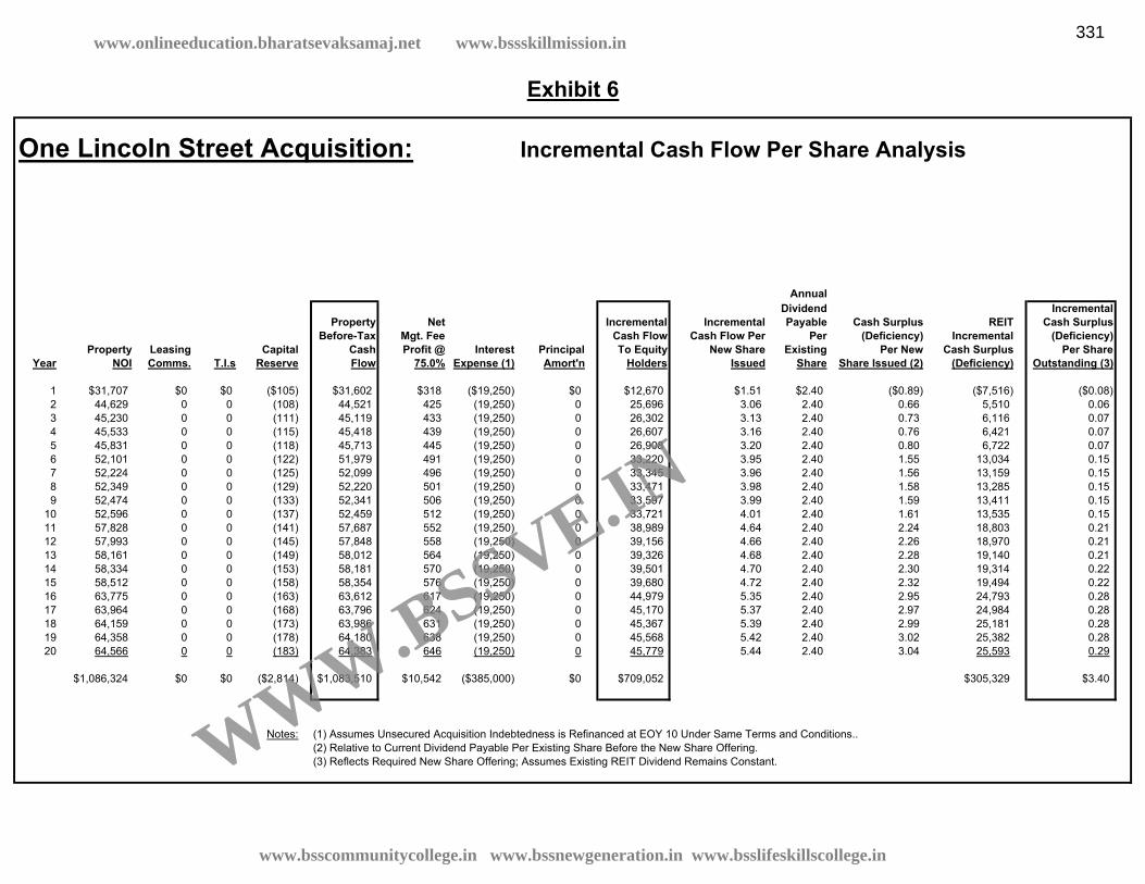
Exhibit 6
One Lincoln Street Acquisition: Incremental Cash Flow Per Share Analysis
Annual Dividend Incremental
Property Net Incremental Incremental Payable Cash Surplus REIT Cash Surplus Before-Tax Mgt. Fee Cash Flow Cash Flow Per Per (Deficiency) Incremental (Deficiency)
Property Leasing Capital Cash Profit @ Interest Principal To Equity New Share Existing Per New Cash Surplus Per Share Year NOI Comms. T.I.s Reserve Flow 75.0% Expense (1) Amort'n Holders Issued Share Share Issued (2) (Deficiency) Outstanding (3)
1 $31,707 $0 $0 ($105) $31,602 $318 ($19,250) $0 $12,670 $1.51 $2.40 ($0.89) ($7,516) ($0.08) 2 44,629 0 0 (108) 44,521 425 (19,250) 0 25,696 3.06 2.40 0.66 5,510 0.06 3 45,230 0 0 (111) 45,119 433 (19,250) 0 26,302 3.13 2.40 0.73 6,116 0.07 4 45,533 0 0 (115) 45,418 439 (19,250) 0 26,607 3.16 2.40 0.76 6,421 0.07 5 45,831 0 0 (118) 45,713 445 (19,250) 0 26,908 3.20 2.40 0.80 6,722 0.07 6 52,101 0 0 (122) 51,979 491 (19,250) 0 33,220 3.95 2.40 1.55 13,034 0.15 7 52,224 0 0 (125) 52,099 496 (19,250) 0 33,345 3.96 2.40 1.56 13,159 0.15 8 52,349 0 0 (129) 52,220 501 (19,250) 0 33,471 3.98 2.40 1.58 13,285 0.15 9 52,474 0 0 (133) 52,341 506 (19,250) 0 33,597 3.99 2.40 1.59 13,411 0.15
10 52,596 0 0 (137) 52,459 512 (19,250) 0 33,721 4.01 2.40 1.61 13,535 0.15 11 57,828 0 0 (141) 57,687 552 (19,250) 0 38,989 4.64 2.40 2.24 18,803 0.21 12 57,993 0 0 (145) 57,848 558 (19,250) 0 39,156 4.66 2.40 2.26 18,970 0.21 13 58,161 0 0 (149) 58,012 564 (19,250) 0 39,326 4.68 2.40 2.28 19,140 0.21 14 58,334 0 0 (153) 58,181 570 (19,250) 0 39,501 4.70 2.40 2.30 19,314 0.22 15 58,512 0 0 (158) 58,354 576 (19,250) 0 39,680 4.72 2.40 2.32 19,494 0.22 16 63,775 0 0 (163) 63,612 617 (19,250) 0 44,979 5.35 2.40 2.95 24,793 0.28 17 63,964 0 0 (168) 63,796 624 (19,250) 0 45,170 5.37 2.40 2.97 24,984 0.28 18 64,159 0 0 (173) 63,986 631 (19,250) 0 45,367 5.39 2.40 2.99 25,181 0.28 19 64,358 0 0 (178) 64,180 638 (19,250) 0 45,568 5.42 2.40 3.02 25,382 0.28 20 64,566 0 0 (183) 64,383 646 (19,250) 0 45,779 5.44 2.40 3.04 25,593 0.29
$1,086,324 $0 $0 ($2,814) $1,083,510 $10,542 ($385,000) $0 $709,052 $305,329 $3.40
Notes: (1) Assumes Unsecured Acquisition Indebtedness is Refinanced at EOY 10 Under Same Terms and Conditions.. (2) Relative to Current Dividend Payable Per Existing Share Before the New Share Offering. (3) Reflects Required New Share Offering; Assumes Existing REIT Dividend Remains Constant.
www.bsscommunitycollege.in www.bssnewgeneration.in www.bsslifeskillscollege.in
331www.onlineeducation.bharatsevaksamaj.net www.bssskillmission.in
WWW.BSSVE.IN

11.432 CMBS Exercise
11.432/15.427J Real Estate Capital Markets Spring 2007
Case 3: CMBS Exercise Due Thurs March 22, in class.
Purpose of assignment:
To give you some basic familiarity with a typical real world CMBS offering from the perspective of the issuer, and to use that as a platform to build your understanding of some fundamental aspects of the
CMBS industry and the real estate capital markets . You may work in groups of up to five. You should prepare a brief narrative report (typed doc max 4 pages plus at most 2 pages of exhibits) plus a PowerPoint presentation (max 5 slides) that your group will be ready to present to the class on the due date (both files should be handed in electronically plus hardcopy to the TA on the due date, with electronic cc to Prof. Geltner). Background In early 2005 General Electric Commercial Mortgage Corporation (GECMC) engaged Deutsche Bank Securities (DBS), a major CMBS investment bank, to launch a new series of CMBS certificates. GECMC is a subsidiary of General Electric Capital Corp (itself a subsidiary of GE Capital Services which is in turn a subsidiary of the giant parent firm, the General Electric Company). GE Capital is a major originator of commercial mortgages, including conduit loans. GECMC wanted to sell a number of recently-issued loans to obtain cash so that GE Capital could originate more commercial mortgages, their primary business. Thus, GECMC had a diversified pool of loans that they hoped would make the core of a good CMBS issue. The pool that was put together consisted mostly of these GE Capital loans, but also included a few other loans from other major commercial mortgage lenders. The overall pool consisted of 127 commercial mortgages secured primarily by first liens on 138 commercial, multi-family and manufactured housing community properties. This included 92 loans from GE Capital, 17 loans from German American Capital Corporation, and 18 loans from Bank of America. The loans were all newly issued (“conduit” loans as opposed to “seasoned” loans), and in aggregate included $1,674,199,523 of outstanding balance (“par value”), collateralized by properties estimated to be worth in total approximately $2,355,000,000. As usual, a trust was established (as a tax-exempt “REMIC” vehicle) to hold the pool of mortgage loans on behalf of the security holders, with LaSalle Bank acting as trustee. A master servicer contract was signed with GEMSA Loan Services (another GE subsidiary), to administer the pool and securities. A special servicer contract was signed with Lennar Partners to handle defaults, workouts, and foreclosures and other such problems that might (would) arise within the mortgage pool. (Lennar is a large, diversified real estate firm who ended up purchasing the so-called “B piece” of the issue, the security classes with credit ratings below the investment grade level of BBB-.) A team of investment banks was put together under the lead of DBS and Bank of America Securities. The securities were designed and structured, and credit ratings were obtained for the securities from S&P, Fitch, and Dominion Bond Rating Service. As required by the SEC
Page 1
www.bsscommunitycollege.in www.bssnewgeneration.in www.bsslifeskillscollege.in
332www.onlineeducation.bharatsevaksamaj.net www.bssskillmission.in
WWW.BSSVE.IN

11.432 CMBS Exercise
for any investment being offered to the public, a prospectus was prepared, dated February 3, 2005, and the public offering was made under the (not very sexy but typical) title of: “GECMC Commercial Mortgage Pass-Through Certificates, Series 2005-C1” (GECMC 2005-C1, for short). The issue closed on February 17. By the standards of the day, this CMBS issue was considered a relatively simple, “plain vanilla” deal. Nevertheless, it might seem complex to the uninitiated. . . A total of 27 classes (or “tranches”) of securities were created from the underlying mortgage pool, including 22 par-valued classes and two IO classes described in the prospectus.* It was decided that 11 of the lower-rated tranches would be sold privately, not included in the public offering but included in the prospectus. The 12 top-rated par-valued classes, all those with a credit rating of “A-” or higher, containing the vast bulk of the loan pool value ($1,550,727,000 par value), plus one of the IO classes, was included in the public offering (13 classes in all). The private placement consisted of the remaining $123,427,000 in par value in 11 classes (including 10 with par values and one IO), with ratings of “BBB+” and lower.†
The Prospectus thus consists of two parts: A basic prospectus relating to the entire issue (24 tranches), and a more specific Supplement relating to the publicly-offered securities only (the front part of the document). The overall structure of the deal is summarized on page S-7 of the Supplement. The publicly-offered classes of securities are described in detail in pages 103-143 of the Prospectus Supplement, with the main description of the prepayment cascade in pp.108-126, and the main description of the credit loss cascade in pp.127-130. The loan pool is detailed in the Annex at the end of the Supplement (and also contained in the downloadable Excel file available on the course web site‡), and is summarized in pp.67-103 of the Supplement, with individual briefs on each of the 10 largest loans (and their underlying properties) on pp.10-65 of the basic Prospectus (after the annexes in the middle of the document). There is also a tabular summary of the pool characteristics at the end of the Annex and on pp.5-7 of the basic prospectus. As with all prospectuses, a major section is devoted to descriptions of the major investment risk considerations that potential buyers of the securities in the public market should be aware of (Supplement pp. 34-66). The subordination structure of the GECMC 2005-C1 securities is typical of CMBS issues of the early 2000s. Of course, credit losses can occur from several sources, including loan payment delinquency, default, and losses in foreclosure (among others). Any credit losses to the pool (coming from any of the mortgages) are assigned first to the bottom tranche (Class P), then to the next lowest (Class O), and so on up the ladder in reverse alphabetical order. Credit losses reduce the outstanding balance (par value) of whichever remaining class of security is lowest until that class is completely wiped out, before the next lowest class becomes exposed. (Reductions in par value commensurately reduce the amount of interest payments the security holders are entitled * The Prospectus mentions but does not describe three classes (L,R, and LR). These have no par value, are not for sale, and simply provide a device for the CMBS issuer to obtain “residual cash flows” in the pool, if any, after all of the other classes have been paid all that is owed to them. In essence, you may think of this CMBS issue including only the 24 classes described in the Prospectus. † The seven lowest of these were bought by Lennar, representing 3.625% of the loan pool par value. ‡ To open the Excel file, skip the password and open as “Read Only”. You can still copy/paste data out of the file into another workbook.
Page 2
www.bsscommunitycollege.in www.bssnewgeneration.in www.bsslifeskillscollege.in
333www.onlineeducation.bharatsevaksamaj.net www.bssskillmission.in
WWW.BSSVE.IN

11.432 CMBS Exercise
to, as the interest owed equals the coupon rate times the par value for each bond.) The “senior classes” (the top seven classes: A-1 through A-5 plus A-AB and A-1A) all have equal subordination and would be docked credit losses on a pro-rata basis if all the subordinate classes were all already wiped out and there were still further credit losses in the pool. Regarding default risk, the senior classes’ initial subordination is 20% (meaning 20% of the initial pool par value is subordinated to the senior securities). Below that Class A-J has 13.375%. All eight of those “A” classes are rated AAA by the credit rating agencies. Below Class A-J, Classes B, C, D, and E have ratings of AA, AA-, A, and A- respectively. Together with Class X-P’s IO securities, this completes the publicly offered securities of the GECMC 2005-C1 issue. The non-offered certificates range from the F Class’ 6% subordination, which warrants an investment-grade BBB+ rating, down to Class O’s 1.5% subordination (B- credit rating) and the first-loss Class P that has no protection (no rating). Regarding maturity and interest rate risk (and prepayment risk), the retirement structure of the deal is “plain vanilla” except that the loans in the underlying pool were divided into two groups. The vast bulk of the loans are in Group 1, which is well diversified by property type. (Group 1 consists of 114 loans with over 91% of the total pool value.) Group 2 is not diversified by property type, consisting of 13 loans that are all secured by apartment properties.* The separation into two groups of loans is made to allow two different streams of principal payment cash flows to separately retire different classes of securities. In particular, payments of principal from the all-apartment Group 2 of loans will go first to the A-1A Class until that class is retired, while payments of principle from the diversified Group 1 of loans will cascade down the A-1 through A-5 classes until they are retired and only then may be available for A-1A if it still exists. Classes A-1 through A-5 will be retired sequentially in order, while Class A-AB will be retired according to a pre-specified schedule between months 60 and 113 (and will have first claim on payments of principal from the Group 1 loans for that purpose). After Class A-5 is retired, subsequent payments of principal will then retire Class A-J and then Classes B through P in alphabetical order. As most of the loans in the pool have a 10-year maturity (two loans have 15 year maturities), this results in contractual weighted average maturities (WAMs) ranging from 2.61 years for Class A-1, down to 9.85 years for Class A-5, and on down to 11.76 years for Class P at the bottom of the principal payment waterfall. A final aspect of the GECMC 2005-C1 issue that is worthy of note is the pass-through coupon rates assigned to each class. These are generally assigned to allow the investment grade classes (Class H and above) to sell at or near par value, while the below investment grade classes are assigned coupon rates approximately equal to the original weighted average coupon rate in the pool. Before beginning the exercises . . . Download the Prospectus pdf file (which includes the Supplement in the front), and look it over briefly (obviously, we don’t expect you to read it in its entirety for this assignment, but get a feeling for the nature of both the document and the security offering). * One loan is backed by a portfolio of three apartment properties in Charlotte, NC.
Page 3
www.bsscommunitycollege.in www.bssnewgeneration.in www.bsslifeskillscollege.in
334www.onlineeducation.bharatsevaksamaj.net www.bssskillmission.in
WWW.BSSVE.IN

11.432 CMBS Exercise
Download the Morgan Stanley CMBS Primer, 5th Edition, and use this (as well as Geltner-Miller Section 18.1 and Chapter 20) as a basic reference as you perform the exercises below. (If you make judgments based on these references, please cite the source in your case write-ups, to assist the TA.) Exercise 1: Gaining familiarity with the loan pool… The most fundamental aspect of any CMBS issue is the loan pool underlying the securities, and the properties collateralizing those loans. As a first exercise, we would like you to examine the loan pool information in the prospectus and in the downloadable “Annex_LoanPool” Excel file. Deliverables: (1) See if you can explain why the largest loan in the pool is represented as having a 63.77% LTV when the loan balance is $97,255,523 and the collateral property (a shopping mall in Michigan) is evaluated at $305,000,000. (2) Use the Excel file to construct histograms (more detailed than the tables in the prospectus) of the frequency distribution of the loans’ LTVs, DSCRs, and Remaining Term to Maturity (or advance payment date), as of the cut-off date of the CMBS issue. (3) Identify the largest loan, the smallest loan, the ones with the longest maturity, and tabulate the percentage of total pool par value that is included in the 10 largest loans detailed in the Prospectus briefs. (4) How many manufactured home community loans are there in the pool, and what fraction of the overall pool value do they represent? Exercise 2: Default Risk… As you know (from lectures and the text, right?...) default risk, and the potential “credit losses” associated with such risk, is a major source of concern for investors in CMBS. This risk (and its perception) can therefore have a large impact on the market value (and hence the prices obtained in the market place) for such bonds. A basic way to think about the amount of default risk in a mortgage based investment is to multiply the probability of mortgage default times the “severity” of the loss in the event of default. Though crude, the result is a kind of “expected credit loss” measure as a fraction of loan value, or, for a pool of mortgages, you could think of it as an expected loss of pool value due to credit events.* The simplest way to measure the probability of mortgage default is by the “lifetime” or “cumulative” default probability for a given mortgage, that is, the probability that the loan will
* This ignores the timing of the defaults within the life of the mortgage(s), and the resulting impact on the investment return or yield. For the interested student, a more in-depth perspective on the impact of credit losses on mortgage (or CMBS) market yields and asset valuation is presented in Sections 18.1 and 19.2 of the Geltner-Miller text (pps.439-448, 475-485). You are not, however, required to read these sections to do this exercise.
Page 4
www.bsscommunitycollege.in www.bssnewgeneration.in www.bsslifeskillscollege.in
335www.onlineeducation.bharatsevaksamaj.net www.bssskillmission.in
WWW.BSSVE.IN

11.432 CMBS Exercise
default at any time during its life, that is, any time prior to its contractual maturity. The simplest way to measure the loss severity is by the percent of outstanding loan balance owed at the time of default that would not be recovered through the foreclosure process. Some historical data that is widely cited in the industry, relevant to both of these measures, is given in the Morgan Stanley Esaki at al study which you can download from the course web site
in the “Esaki_REF2002” pdf file (see the Class Resources section of the Materials page).* Exhibit 6B of this report is reproduced here. Each bar in the exhibit shows the percentage of commercial mortgages issued in the year indicated on the horizontal axis, which experienced a default at some point in the loan life (up to the cutoff date of the study at the end of 2000).† For example, the worst cohort was the loans issued in 1986, 27.7% of which had defaulted by the end of 2000. On the other hand, only 9.3% of the loans originated in 1977 ever defaulted. The overall average lifetime rate across all of the loan cohorts in Exhibit 6B is 16.4%.‡ The Esaki * An updated version of this study is presented in Chapter 12 of the Morgan Stanley CMBS Primer, 5th Edition, which is also available in the Class Resources section of the course web site. And an updated version of the study is discussed in the Geltner-Miller text Chapter 18 (see section 18.1.3, pp.443-448). However, for this exercise let’s use the 2002 REF article whose results are presented in the chart above. † Note that the data source for the Morgan Stanley studies was the loan pool of the American Council of Life Insurers (ACLI). These are whole loans held in life insurance company portfolios. Thus, their default experience may be different from that of conduit loans, which are a much more recent phenomenon. ‡ Note however that the more recently issued cohorts would not have had time to complete their entire lifetime default behavior by the end of the data cutoff in 2000. This is one reason the most recent cohorts have such a low default rate. Nevertheless, this data truncation cannot explain most of the recent decline in default rates, as historically almost half of all commercial mortgage defaults occur within the first five years of loan life. In fact, subsequent to the disastrous experience of the late 1980s and early 1990s commercial mortgage underwriting standards became stricter. This combined with a booming real estate market (either in the space market or the asset market, or both) in the late 1990s and early 2000s has given commercial mortgages a much better default performance record in recent years.
Page 5
www.bsscommunitycollege.in www.bssnewgeneration.in www.bsslifeskillscollege.in
336www.onlineeducation.bharatsevaksamaj.net www.bssskillmission.in
WWW.BSSVE.IN

11.432 CMBS Exercise
study found an overall average loss severity of 34%, meaning that among loans that defaulted, the average losses (in expenses, foregone interest, and lost principal) equaled 34% of the loan outstanding balances. A crude but interesting way to understand the credit loss risk exposure of a CMBS issue is to apply expected credit loss analysis to the tranches in the issue. This can be done in a sensitivity analysis framework to gain insight about the nature of the credit loss risk the CMBS securities face, as a function of their credit ratings. We would like you to perform such an exercise on the GECMC 2005-C1 issue here… Deliverables: (1) Multiply the Esaki overall average lifetime default rate times the Esaki overall average loss severity to obtain a sort of overall average credit loss factor, a type of average expected losses among commercial mortgages. Then apply this loss factor to the GECMC 2005-C1 securities, from the bottom up (based on their subordination credit support), and tell us which tranches (which classes of securities) would be completely wiped out by such “average” credit losses, and which class of securities would be the bottom one affected at all, and what is its bond credit rating. (2) Repeat the exercise (1) above only now model a “worst case” scenario in which the lifetime default rate of the worst historical cohort in the Esaki study happens again. (3) Repeat the exercise again, only now assume that the default experience will be that indicated in the most recent five cohorts (1991-95) in Exhibit 6B. (4) Present your findings here in a simple well designed PowerPoint graphic.*
* You may (but need not if you have a better idea) model this on the graphic in class lecture notes entitled “Conduit Capital Structure vs ELS Study” (approximately Slide #36).
Page 6
www.bsscommunitycollege.in www.bssnewgeneration.in www.bsslifeskillscollege.in
337www.onlineeducation.bharatsevaksamaj.net www.bssskillmission.in
WWW.BSSVE.IN

11.432 CMBS Exercise
Exercise 3: Pricing the Securities… The “bottom line” in any CMBS issue is the pricing of the securities. The most important and fundamental measure of the success of the issue is the gross profit (you can think of it as “NPV”) generated by the difference in the aggregate price of the CMBS securities issued minus the cost of the mortgages placed into the pool. This profit represents the economic value created by the CMBS issuance, and from this gross profit the administrative costs and overhead and required profit margins of all of the various entities that participate in the creation and issuance of the CMBS securities must be obtained.* Here we want you to go through a somewhat simplistic (and only approximate), but illustrative and hopefully instructive, exercise of pricing the 24 tranches of securities created in the GECMC 2005-C1 issue. To perform this exercise you will need to create a table in Excel in which each of the security classes is a row in the table, with much of the summary information from the table on page S-7 of the Prospectus Supplement entered in columns. You should be able to price each security class separately in the Excel worksheet. To do this, you will work with the fundamentals:
(i) The price of each security class is the present value of its expected (contractual) future lifetime cash flow stream discounted at the market yield to maturity applicable to that class;
(ii) (ii) The (contractual) cash flow stream is determined by the Class’ initial par value, its coupon (“pass-through”) rate (determines the interest), and its contractual maturity as indicated in the “Principal Window” column of the Summary table on page S-7 (determines the payout of principal balance in the tranche);
(iii) (iii) The market yield to maturity applicable to each class is a function of the default risk of the tranche (as indicated by its credit rating) and by its maturity as indicated by its weighted average life and the slope of the current yield curve in the bond market.
Deliverables: (1) Expand your Excel table 180 columns out to the right to represent the 180 future months envisioned in the contractual lifetimes of the mortgages in the pool (note that the end of the longest principal window is 180 months for Class P, reflecting the fact that there are a couple of 15-year mortgages in the pool†). Assume that only interest is received by each tranche until the beginning month of its “Principal Window”, and that the tranche is completely retired by the end of its Principal Window. For simplicity (and because it is probably approximately correct), assume that for each tranche the principal is amortized during the Principal Window by a monthly payment level annuity in arrears (i.e., of the type for which the Excel PMT(coupon/12, EndWindowMonth – BegWindowMonth, Par$) function can be used. For simplicity, assume that
* It should be noted that apart from the net difference between the cost of the loan pool and the gross proceeds from the sale of the securities based on it, there is another potential source of profit to the CMBS issuer, namely “residual cash flows” in the pool, that is, extra cash flow that none of the 24 security classes described in the Prospectus are entitled to. † But please note: In general specific mortgages are not assigned to any specific classes of securities. The mortgages are completely “pooled” in the trust, and the securities get their cash from the trust. In the case of GECMC 2005-C1 there is some differentiation within the pool into the “Group 1” and “Group 2” loans, for purposes of (contractual) principal repayment. But this is sufficiently accounted for in the “Principal Window” indicated for Class A-1A in the table on page S-7. You need not (and should not) worry about assigning any specific mortgages to any specific classes in this exercise.
Page 7
www.bsscommunitycollege.in www.bssnewgeneration.in www.bsslifeskillscollege.in
338www.onlineeducation.bharatsevaksamaj.net www.bssskillmission.in
WWW.BSSVE.IN

11.432 CMBS Exercise
for the IO tranches the cash flow in the first month equals the notional par value times the notional coupon rate (divided by 12), and then assume this cash flow declines linearly over the
entire Principal Window of 120 months (reflecting the reduction in excess interest as par value is retired from the pool).* The result should be a 24X180 cell table of future contractual cash flow projections for the certificate classes. (2) Develop estimates of the market yields for each security class, based on the currently prevailing CMBS yield spreads and the currently prevailing yields in LIBOR Swaps and U.S. Treasury Bonds. You can do this using the spreads information for the six major fixed-rate credit ratings in the “CMBS Spreads” table below (taken from the February 4, 2005 issue of Commercial Mortgage Alert).† For simplicity (and consistency) assume that the relevant current yields are 4.3% for 5-year Swaps, 4.7% for 10-year Swaps, 3.7% for 5-year T-Bonds and 4.1% for 10-year T-Bonds; and assume that the yield curve is linear over the relevant range.‡ Assume that a “+” rating reduces the spread by 2 basis points, and a “-“ rating increases the spread by 2 basis points. Assume that the spread for the Non-Rated Class P is 1200 bps, and for the two IO classes it is 150 bps. The result should be a table presenting your estimated market yields for each of the 24 tranches. (3) Apply the Excel NPV(yield/12, CFrange) function using the cash flows and yields you calculated in steps (1) and (2) above to derive an estimated market value for each of the 24 tranches.
* In reality the IO cash flow stream would be a bit more complicated than this. Also, the Class A-AB principal is retired according to a pre-specified schedule (in Annex 5 of the Prospectus Supplement). But we will ignore these subtleties in this exercise. † Use the 2/1 spreads in the first column. ‡ The bond market “yield curve” is explained in Geltner-Miller section 19.1.3 (pp.469-471), and is reported daily in the Wall Street Journal and web sites such as www.smartmoney.com. Usually shorter maturity bonds have lower market yield rates. Here in this exercise we are simplifying the yield curve while retaining its essence. As instructed here, for example, the yield for a bond with WAM of 2.5 years would be: 4.7% - (10-2.5)(4.7%-4.3%)/5 = 4.1% for a Swap; or 4.1% - (10-2.5)(4.1%-3.7%)/5 = 3.5% for a T-Bond. To this you would need to add the default risk premium spread indicated in the “CMBS Spreads” table from CMA. For bonds of rated above BBB+, the spread is added to the appropriate maturity Swap yield; for bonds BBB+ and below the spread is added to the appropriate maturity T-Bond yield. For our purposes in this exercise, assume that the Swap spread for any AAA bond less than 7.5 years WAM is the 19 bps indicated for the 5-yr average life, and for any AAA bond of longer maturity it is the 22 bps indicated for the 10-yr average life. (For this purpose assume the IO tranches have a 5-yr WAM.)
Page 8
www.bsscommunitycollege.in www.bssnewgeneration.in www.bsslifeskillscollege.in
339www.onlineeducation.bharatsevaksamaj.net www.bssskillmission.in
WWW.BSSVE.IN

11.432 CMBS Exercise
(4) Total the estimated market values across the 24 tranches and compare the resulting aggregate market value for the issue to the aggregate loan pool outstanding balance (par value). What is the resulting estimated gross profit (or loss) from the security issue, assuming that the loan pool actually cost its par value to acquire.* Add an additional $40,000,000 of present value of profit expectation to reflect private residual tranches held by the issuers, to get the overall profit up to typical magnitudes.
* In reality this might not be the case. For example, if market interest rates have increased since the loans were issued the pool might be acquired for less than its aggregate par value. Also, in the primary market (from the perspective of the mortgage originators who are selling the loans into the pool), up-front fees and discount points in the mortgages could have caused the actual cost of issuing the loans to be less than their initial par values (initial outstanding principal balances). On the other hand, if interest rates have fallen since loan issuance, the pool might cost more than its aggregate par value. And keep in mind that the administrative and overhead costs and required profit of the intermediary and servicing agents must be paid from the gross profits (e.g., the investment bank fee). Note however that the quoted pass-though coupon rate is net of a service charge that is taken out of the pool cash flow each month to pay the regular servicing and administrative costs of the trust.
Page 9
www.bsscommunitycollege.in www.bssnewgeneration.in www.bsslifeskillscollege.in
340www.onlineeducation.bharatsevaksamaj.net www.bssskillmission.in
WWW.BSSVE.IN

11.432 CMBS Exercise
Exercise 4: Gaining Some Perspective… The CMBS market has evolved in a rather interesting manner over the past several years. Similar to other aspects of the real estate capital markets and asset markets, the commercial mortgage and CMBS markets are much more aggressive and “expensive” than they were a few years ago. Down on Main Street, loan originators are being more aggressive in their underwriting (that is, applying loan approval conditions and terms that could result in more risk in the loans), though this is still a far cry from what was going on in the mid-to-late 1980s. On Wall Street, CMBS subordination levels have come down dramatically. (See the Exhibits below.) Thus, less credit support is now being required by the credit rating agencies to receive a given credit rating. Furthermore, CMBS spreads have narrowed, especially recently, to levels not seen since before the financial crisis of 1998.*
CMBS Spreads Over 10-Year Treasury: Investment Grade
0
50
100
150
200
250
300
350
Aug
-96
Nov
-96
Feb-
97M
ay-9
7A
ug-9
7N
ov-9
7Fe
b-98
May
-98
Aug
-98
Nov
-98
Feb-
99M
ay-9
9A
ug-9
9N
ov-9
9Fe
b-00
May
-00
Aug
-00
Nov
-00
Feb-
01M
ay-0
1A
ug-0
1N
ov-0
1Fe
b-02
May
-02
Aug
-02
Nov
-02
Feb-
03M
ay-0
3A
ug-0
3N
ov-0
3Fe
b-04
May
-04
Aug
-04
Nov
-04
Bas
is p
oint
s
0
50
100
150
200
250
300
350
Aaa Aa A
* See Geltner-Miller section 20.3.4 (pp.509-512) for a description of the 1998 financial crisis and the CMBS market at that time.
Page 10
www.bsscommunitycollege.in www.bssnewgeneration.in www.bsslifeskillscollege.in
341www.onlineeducation.bharatsevaksamaj.net www.bssskillmission.in
WWW.BSSVE.IN

11.432 CMBS Exercise
CMBS Spreads Over 10-Year Treasury: Non-Investment Grade
0
100
200
300
400
500
600
700
800
900
1000
1100
Aug
-96
Nov
-Fe
b-97
May
-A
ug-9
7N
ov-
Feb-
98M
ay-
Aug
-98
Nov
-Fe
b-99
May
-A
ug-9
9N
ov-
Feb-
00M
ay-
Aug
-00
Nov
-Fe
b-01
May
-A
ug-0
1N
ov-
Feb-
02M
ay-
Aug
-02
Nov
-Fe
b-03
May
-A
ug-0
3N
ov-
Feb-
04M
ay-
Aug
-04
Nov
-
Bas
is p
oint
s
0
100
200
300
400
500
600
700
800
900
1000
1100
Ba B This means that investors buying CMBS are paying higher prices, in effect, for a given credit rating. In part, this certainly reflects the recent more favorable experience with commercial mortgage default, as indicated earlier in our discussion in Exercise 2 (for example in the Esaki studies). An in part it reflects the capital markets’ newly acquired appetite for real estate investments of all types, and the resulting flow of capital into both debt and equity real estate investments. Nevertheless, capital markets have been known to change and reverse directions quickly in the past, and it could happen again. In this exercise we would like for you to use the historical experience surrounding the 1998 financial crisis to see what would happen to the profitability of a CMBS issue such as GECMC 2005-C1 if conditions in the capital markets suddenly changed to levels experienced in the not-too-distant past. . . Deliverables: (1) Reprice the securities in the GECMC 2005-C1 issue holding everything as before (including credit rating, coupon rates and yield spreads, and the total amount of loans in the pool, and also including the $40,000,000 residual profit), only now suppose that this issue had to be structured using the credit support subordination levels that prevailed in 1998, according to Table 1 below. In performing this exercise, you will have to recalculate the amount of the pool’s par value that will be assigned to the securities in aggregate within each of the six major credit rating levels (AAA, AA, A, BBB, BB, B).* What is the new aggregate market value for the issue as a whole? * In performing this exercise, hold constant the proportion of each class within each major credit rating category. For example, previously the total par value of the eight classes with AAA ratings (Classes A-1 through A-J) was: (100% – 13.375%)($1,674,200) = $1,450,275 (in thousands). Now it will be: (100% – 29%)($1,674,200) = $1,188,682. However, the proportion within that AAA total assigned to each class will remain the same. Thus, Class A-1 was $75,842 / $1,450,275 = 5.23%, and so it will now be: (.0523)($1,188,682) = $62,162 (thousands). Similarly, the two AA classes (Classes B and C) were (13.375% – 9.875%)($1,674,200) = $58,597 (thousands) both together. Now they will be: (29% – 24%)($1,674,200) = $83,710 (thousands).
Page 11
www.bsscommunitycollege.in www.bssnewgeneration.in www.bsslifeskillscollege.in
342www.onlineeducation.bharatsevaksamaj.net www.bssskillmission.in
WWW.BSSVE.IN

11.432 CMBS Exercise
How does this compare to your answer in Exercise 3 (Question 4)? In other words, how much value has been “created” by the credit rating agencies (as representatives of the bond market?) having “decided” that less credit support is necessary in CMBS issues (for a given credit rating), in other words, in effect, that commercial mortgages are less risky than the market previously thought? (Think about how much value could be “lost” if the market changed its mind and went back to the previous perception.) Table 1
Subordination for Conduit/Fusion Transactions
1As of August 19, 2004Source: Morgan Stanley, Commercial Mortgage Alert
AAA
AA
A
BBB
BB
B
CCC
1998
29%
24%
18%
13%
6%
3%
2%
1999
27%
22%
17%
12%
6%
3%
2%
2000
23%
19%
14%
11%
5%
3%
2%
2001
21%
17%
13%
9%
4%
2%
2%
2002
20%
16%
12%
8%
4%
2%
2%
17%
14%
10%
7%
3%
2%
1%
2003
14%
12%
9%
5%
3%
2%
1%
2004 1
(2) Perform the same exercise as in (1) above, holding everything constant only now apply not only the 1998 credit support subordination levels, but also the April 1998 yield spreads, as indicated in Table 2 below.* Thus, you are pricing the GECMC 2005-C1 securities based on current 2005 interest rates, but with 1998 subordination levels and April 1998 yield spreads, just prior to the 1998 financial crisis. Note not only the aggregate value of the total of all of the securities, but also note in particular the value of the three “B” rated tranches (Classes M,N,O). (3) Finally, perform the same exercise as in (2) above, only now apply the yield spreads of December 1998, reflecting the financial crisis of that year. Compute the total aggregate market value of all the securities, and compare this against the pre-crisis value you computed in (2) above. How much of a hit did the value of the entire issue take as a result of the crisis (both in absolute dollars and in percent of the aggregate issue value)? Perform the same comparison for the three B-rated classes (M,N,O). What percentage of the B classes’ value has been lost. Suppose you were an investment bank specializing in CMBS like Nomura Securities at that time in 1998. Because of your confidence in your knowledge of the market, you were holding a huge * Note: the yield spreads in Table 2 are quoted relative to 10-year U.S. Treasury Bonds for all rating levels. Hold the T-Bond yield rates and yield curve assumption as before in Exercise 3, in effect, work with 2005 interest rates. We want you to see the pure effect of changing yield spreads (and subordinations in the previous question) holding everything else constant.
Page 12
www.bsscommunitycollege.in www.bssnewgeneration.in www.bsslifeskillscollege.in
343www.onlineeducation.bharatsevaksamaj.net www.bssskillmission.in
WWW.BSSVE.IN

11.432 CMBS Exercise
quantify of highly levered investments in such B-rated securities. Do you see how you could be completely wiped out and bankrupted by such a “crisis” in the financial markets?*
Table 2: CMBS Mkt Yld Spreads (bps) over 10-yr T-Bonds
Dec.2004 Dec.1998 Apr.1998 AAA 70 136 77 AA 77 161 88 A 85 186 105 BBB 127 275 140 BB 325 575 250 B 770 825 450
* Of course, this is exactly what did happen to Nomura Securities in 1998. Recall, furthermore, that the crisis of 1998 was not at all based in any fundamental problem in the real estate space or capital markets. Rather, it was caused by a default by the Russian government and a resulting panic that caused a “flight to quality” in the world bond markets, which bid up the price of U.S. Treasury Bonds and at least temporarily dried up the liquidity in other bond markets, especially for low-credit bonds.
Page 13
www.bsscommunitycollege.in www.bssnewgeneration.in www.bsslifeskillscollege.in
344www.onlineeducation.bharatsevaksamaj.net www.bssskillmission.in
WWW.BSSVE.IN

Fairweather Pension Plan
In this case, you are to play the role of Leslie Rentleg, an independent investment consultant specializing in providing institutional investment clients, such as pension funds and endowment funds, with strategic advice regarding “core” portfolio allocations. (The portfolio “core” refers to the main component of professional investment portfolios the allocation of which is usually analyzed using Modern Portfolio Theory.) You should work in teams of 3 students each. (If necessary, a few 2-person teams will be permitted, but no 4-person teams.) Each team should prepare a PowerPoint presentation and a 2-page Word file executive summary covering all four of the “scenes” in the case. On the due-date of the case, teams will be selected randomly to present in class each of the scenes, using your PowerPoint presentation for that scene (a different team will be randomly selected for each scene). All teams should hand in to the TA printouts of their PowerPoint files (6 slides to the page), as well as a printout of their Word file executive summaries.*
Background: It had taken Leslie almost an hour and a half to navigate the Audi A4 Quattro through yet another Boston snowstorm that was timed perfectly for the morning commute. He was beginning to wonder why he had bothered, when he received a call from Cate Polleys, Director of Real Estate Research for Fidelity Investment Management, just down the street. Cate was trying to land a new client, the pension fund of Fairweather Corporation, a major manufacturing firm in the packaging industry. Cate was hoping that Leslie’s expertise and experience could be helpful to her in convincing Fairweather that Fidelity was the right firm to provide strategic advice for the firm’s defined-benefit plan’s investment portfolio allocation decision. Fairweather had recently had a major change in management. A closely held family firm, the original founder had recently stepped aside in favor of a professional management team, including a new CFO by the name of Clayton Patrick. Clayton had been surprised to learn that Fairweather’s pension plan was 100% in bonds. He believes that “a pension plan should be managed so as to maximize return within well-defined risk parameters,” and “anyone can buy bonds and sit on them”. Clayton contacted Cate, who convinced him that Fidelity should be one of a short list of investment management firms that Fairweather should consider hiring to assist with both planning and implementation of a more broad-based and profitable policy for the firm’s pension fund. What Cate wanted from Leslie was an overview of the portfolio allocation implications of “Modern Portfolio Theory” (MPT). Cate knew that strategic investment decision making needed to consider other issues besides those treated in MPT, but she felt that this rigorous scientific model would be a good starting point and frame of reference for an objective discussion with Fairweather’s CFO. Also, Cate felt that one of Fidelity’s comparative advantages relative to their competition was their expertise in including a full range of investment asset classes in clients’ portfolios, going beyond just the traditional but narrow asset classes of stocks and bonds. (Surely her boss, Linda Valerie, didn’t really say: “Portfolios of only stocks and bonds are sooo 20th * At the discretion of the TA, electronic submission may be substituted for hardcopy. Check with the TA.
1
www.bsscommunitycollege.in www.bssnewgeneration.in www.bsslifeskillscollege.in
345www.onlineeducation.bharatsevaksamaj.net www.bssskillmission.in
WWW.BSSVE.IN

century,” - but the point was well taken.) Cate was proud of Fidelity’s ability to include real estate as a third major asset class in the portfolio, even for funds as small as Fairweather’s, by the use of various types of real estate securitization, both public and private, and even use of the new real estate equity derivatives. (For example, nowadays there were not just separate accounts and commingled funds for direct investment in private real estate, but “funds of funds”, private REITs, and a growing array of private equity vehicles, as well as the fascinating new possibility of index return swaps.) Cate had already done some background research on Fairweather, which she summarized for Leslie. Fairweather is the eighth largest domestic packaging company, with annual revenues of $500 million. Revenues have grown about 8.0% per year over the past seven years, with only one down year. The company employs about 7,000 people, compared with 6,500 seven years ago. The annual payroll is about $300 million. Company profits last year were $20 million, compared with $12 million seven years ago. Pension assets are currently $100 million, invested entirely in bonds. The average age of the pension eligible work force is 38 years. Leslie felt that this average age was slightly on the young side, suggesting a relatively long average holding period for Fairweather’s pension fund investments. Leslie agreed to meet Cate next Monday to present her with a preliminary portfolio analysis. Leaving his donut and coffee half finished, he got right on the case… Scene I: Preparation for Monday Meeting with Cate Based on discussions with Cate considering the size and sophistication of Fairweather’s financial staff, Leslie decided to explore a relatively simple six asset class portfolio for Fairweather. The analysis would consider large stocks, small stocks, international stocks, long-term bonds, intermediate-term bonds, and REITs. Leslie decided to base the initial analysis on the historical returns that had actually been achieved by these six asset classes during the 1985-2006 period, analyzing the calendar year annual-frequency periodic total returns achieved.*
For the traditional asset classes of stocks and bonds, Leslie already had the historical investment performance data at hand in an Excel® file, using indices that are widely employed in the investments industry. Leslie would use the Ibbotson Associates “Stocks, Bonds, Bills, & Inflation” (SBBI) historical total return indices to represent large stocks (S&P500) and small stocks. He would use the Lehman Brothers Government/Credit bond indexes for long-term and intermediate-term bond performance. (These indexes represent periodic total returns, or “holding period returns” – HPRs – the returns faced by portfolios regularly marked to market value, not the buy-and-hold-to-maturity return indicated by bond yields.) And Leslie would use the benchmark Morgan Stanley “EAFE” (Europe, Australia, Far East) Index for international stocks.†
* “Total” returns include both current income paid out as well as the change in the asset value each period. Annual frequency returns are accumulated within each year by compounding higher frequency returns such as quarterly or monthly, or by considering the year-over-year percentage change in a cumulative index level. † The historical returns data for these five indexes is provided on the downloadable Excel file posted to the class MIT Server site. Note that the EAFE Index returns are based on US dollars, and so reflect the foreign exchange rate risk inherent in unhedged overseas investment. (The Excel file also contains worksheets for converting monthly or quarterly returns to annual.)
2
www.bsscommunitycollege.in www.bssnewgeneration.in www.bsslifeskillscollege.in
346www.onlineeducation.bharatsevaksamaj.net www.bssskillmission.in
WWW.BSSVE.IN

As Leslie’s familiarity with REIT investment returns data was a bit rusty, he decided to first check out the NAREIT web site (www.nareit.org), to explore what sort of historical returns data were available on that site. One thing Leslie wanted to think about was whether to use the NAREIT All REIT Index or the NAREIT Equity REIT Index to represent the returns to the real estate asset class in his portfolio analysis. (Leslie knew that the main difference was the rather specialized breed of REITs that invest with very high leverage in mortgage assets and risky CMBS tranches, and he was pretty sure Cate wanted to present the REITs asset class with its “best foot forward”.) For his Monday meeting with Cate, Leslie wanted to generate a Markowitz (mean-variance) efficient frontier based on a choice set consisting of the six risky asset classes noted above.* † After presenting a table that showed his expected return inputs (mean, volatility, correlations) for and among all the asset classes, he summarized the frontier in another table that specifically showed the efficient portfolio composition and risk and return statistics for five different risk/return points along the frontier, at target returns spanning the range of what was provided by the individual asset classes.‡ For each target return, the table showed the share of the efficient portfolio in each of the six asset classes (if any), and the expected return and volatility (standard deviation of return) of the portfolio. Leslie also depicted the efficient frontier visually by generating a frontier “area chart” (portfolio composition), which he copy/pasted into a PowerPoint file for his presentation to Cate.
* Believe it or not, Leslie actually had an Excel workbook of templates that he had saved from the CD that came with the textbook he used in his days as a student at the MIT/CRE, that could be used for a portfolio optimization analysis with up to 14 assets or asset classes in the portfolio, based on the Excel Solver. The file repeatedly calls up the Solver utility automatically to fire off an entire “efficient frontier” of portfolios all at once. Leslie also still had his PowerPoint lecture notes covering Chapter 21 of the finance course text, which explained MPT and what the Excel files were actually doing (though of course Leslie had long since sold the actual textbook into the used book market to recoup a miniscule portion of his MIT tuition). † Note that it is sometimes necessary to “reset” the Excel spreadsheet before running the Solver, by entering either zeros or all equal shares in the policy weights row. The point is to make the Solver start searching again for a new optimum. The Solver is a numerical algorithm that works by trial and error. It can sometimes “get stuck”, and needs a sort of “kick” to get it moving. Also note that in the given Excel file with the automatically-solved frontier, you must repeatedly click on the “Optimize” button five times to map out the efficient frontier on five points, and if the macro does not work, you can manually run the Solver repetitively for each point you want on the frontier. Occasionally the Solver will give anomalous results at the extreme ends of the feasible return range (with target return equal to the minimum or maximum return among all the potential constituent assets – points at which the portfolio must consist 100% of the minimum or maximum return asset alone). Finally, note that the portfolio with target return equal to that of the minimum-return asset will not necessarily be the minimum-variance portfolio and therefore not necessarily on the efficient frontier (it will be below the “nose” of the leftward-bending curved frontier). However, you can ignore this fine point in this exercise. ‡ Use points defined by target returns equally spaced between the mean returns of the minimum and maximum return asset classes. With only 6 asset classes in the analysis, “extra” asset class slot(s) in the template (up to 14) must be filled in with “dummy data” such that the extra asset class(es) would not appear in the optimal portfolio. This can be done by giving them artificially very bad return performance (very low negative mean, high volatility, and perfect positive correlation with the other asset classes). The given Excel file initially has such data filled in, but you will need to override or replace some of that depending on how many asset classes you have. Also, when you copy/paste historical return data into the “DATA & STATS” worksheet, take care that you don’t leave any excess old data not written over or erased at the bottom.
3
www.bsscommunitycollege.in www.bssnewgeneration.in www.bsslifeskillscollege.in
347www.onlineeducation.bharatsevaksamaj.net www.bssskillmission.in
WWW.BSSVE.IN

Scene I: Monday Meeting with Cate Leslie’s Monday meeting with Cate went pretty well. However, Cate had a couple of constructive suggestions to improve the analysis. First, she noted that REITs are very similar to “small cap value stocks”, that is, relatively small-capitalization stocks that tend to have high dividend yields and/or high book/market value ratios, stocks that by those measures might be considered to be traditionally “under-valued” in the stock market (and thereby to provide high returns). As there are numerous mutual funds and benchmark indexes that specialize in, and track, the small-cap value stock sector, Cate felt it would make sense to also include an index of the performance of this investment “style” in the portfolio analysis, as small-cap value stocks might act as a potential substitute for REITs in the portfolio. Cate therefore suggested that instead of using one small-cap stock index in the analysis, Leslie should replace the Ibbotson Small Stock index with two more specialized small stock indexes: the Russell 2000 Value Stock Index, and its alter-ego, the Russell 2000 Growth Stock Index. (“Growth stocks” are just the opposite of “value stocks”, stocks with low dividend yields and high price appreciation orientation, often including low book/market value ratios and high price/earnings ratios.) Cate’s other suggestion was potentially even more important. She pointed out that there are really two rather different types of real estate investment vehicles: the publicly-traded REITs that Leslie had considered, but also private investment directly in the underlying property assets, which Leslie had ignored. Cate pointed out that private direct real estate investment was possible even for smaller pension funds nowadays, using private “securitization” vehicles such as co-mingled real estate funds (CREFs), or one of the newer “fund of funds” that allows even smaller denominated investments in diversified portfolios of property by pooling CREF units and issuing smaller-denominated interests in the pool. In fact, recent developments in the investment industry effectively enable highly diversified “synthetic” investment in direct private real estate with greater liquidity and at relatively low transaction costs via derivatives, such as “index return swaps”, which pay off periodically based on indexes of real estate investment returns.* Cate suggested that the National Council of Real Estate Investment Fiduciaries (NCREIF) Property Index (NPI) would be a good benchmark to use to represent the historical periodic investment performance of the direct private real estate asset class. Cate also suggested that, since each of the other two broad asset classes in the portfolio (stocks and bonds) was represented by at least two “sub-classes” (stocks now by four: large cap, both value and growth small cap, and international, while bonds would be represented by both long-term and intermediate-term indexes), it was a bit “unfair” to represent the real estate asset class by only one index. Such an arbitrary asymmetry of “granularity” in the portfolio asset class choice set could bias the result against the asset class that was less well represented by sub-indices. Considering that the underlying real estate assets in the economy make up roughly as much market value as each of the other two broad classes (stocks as a whole and bonds as whole), it seemed only reasonable to represent real estate by at least two sub-classes of investment vehicles.
* For more information about this possibility, see the Geltner & Pollakowski (2006) white paper about the new RCA-based index developed at MIT. The paper is downloadable from the MIT/CRE web site at: http://web.mit.edu/cre/research/credl/rca.html. Derivatives will be covered in the 11.434 “Advanced Topics” course taught in the second half of the spring semester.
4
www.bsscommunitycollege.in www.bssnewgeneration.in www.bsslifeskillscollege.in
348www.onlineeducation.bharatsevaksamaj.net www.bssskillmission.in
WWW.BSSVE.IN

Well, of course, Leslie could have kicked himself for not recognizing Cate’s point earlier by himself. Now he was afraid he had made a bad impression. Leslie realized that the private property market is not perfectly correlated with the REIT market, because Leslie knew that REITs often trade at time-varying premia and discounts to their "net asset values" (NAV). In effect, the stock market (where REIT equity trades) and the private property market (where the underlying properties trade directly) do not always agree about the value of real estate, and this “disagreement” varies over time. (Also, firm level effects such as management actions, agency concerns, capital structure, property development and trading, and other REIT activities, may influence REIT firm equity value and stock returns in ways that may differ from those of the underlying “bricks and mortar”.) Thus, including private direct real estate in the portfolio asset class choice set should improve on the efficient frontier possibilities, allowing greater diversification. Leslie was determined to impress Cate better the next time around. They arranged to meet the following Wednesday after Leslie had incorporated the private direct real estate asset class into the analysis. Scene II: Preparation for Wednesday Meeting with Cate As with the NAREIT data previously, Leslie’s first step was to go to the NCREIF web site (www.ncreif.org), and familiarize himself with the nature of the private real estate investment returns data.* He saw how it was possible to use NCREIF’s query screens to generate “custom indices” consisting of particular types of properties in particular geographic locations, and how the returns indices could be generated based on either value-weighting or equal-weighting of the constituent property returns (the former being the “official” NCREIF method), and with income and appreciation return components computed based either on NOI or cash flow, the former subtracting capital expenditures from the appreciation component instead of from the income component (which is the official NCREIF method).†
To prepare for his Wednesday meeting with Cate, Leslie produced tabular and area chart representations of the efficient frontier and target return portfolios exactly as he had before (including also a table of the input assumptions), only now with eight asset classes including private real estate as represented by the NCREIF Index. Leslie summarized the general characteristics of the efficient frontier with a brief discussion (in executive summary format, both in his PowerPoint presentation and in a hardcopy Word file he prepared for Cate). In this summary Leslie made particular mention of the nature and role of the real estate asset classes in the efficient frontier.
* Get the username and password for accessing the NCREIF web site from the TA or Professor Geltner. You will want to download the total return history using the “custom data query” feature of the web site. When you get into the Member Data Access area of the NCREIF web site, go to the NCREIF Property Index (NPI) Data Products area and then to the NPI Custom Query Screen to add a query to download the returns data history that you want. For our present purposes, the official (default) All properties NPI calendar year total returns will suffice. † While you should use the “official” NPI definitions in the present exercise, keep in mind that an equal-weighted index is arguably superior from a statistical perspective if the index is viewed as a “sample” representing a larger population. The NCREIF property population is less than $300 billion worth out of perhaps ten times that much value in commercial property in the U.S. that is similar in size and quality to the “institutional” properties held by NCREIF members. While the NCREIF population may indeed represent a “universe” of all of the pension fund investment managers who are members of NCREIF, it is not the complete commercial property “universe” in the U.S. It should also be noted that the cash flow based definition of return components, rather than the “official” NOI-based definition, provides a break-out between income and appreciation return components that is more comparable to that in stock market indexes (although this does not matter in the present context as the total return is unaffected).
5
www.bsscommunitycollege.in www.bssnewgeneration.in www.bsslifeskillscollege.in
349www.onlineeducation.bharatsevaksamaj.net www.bssskillmission.in
WWW.BSSVE.IN

Scene II: Wednesday Meeting with Cate The Wednesday meeting went better than Monday’s. Indeed, reflection on the real estate role in the efficient frontier led Cate and Leslie to brainstorm a bit about what was going on, and whether they ought to explore the analysis further. They were both troubled by the difference between the results implied by the MPT analysis based on the historical performance data, and the typical makeup of real world pension portfolios, which they knew had on average less than 5% in real estate, with most small funds like Fairweather having no real estate allocation at all. They were not really satisfied with the data Leslie was using in the inputs of his optimization. Perhaps the NCREIF Index was presenting a biased picture of real estate risk and return, more favorable than real estate really presents, they wondered. It is well known that the NPI is based on appraised values of the constituent properties, and this can make the index artificially “smooth” and “lagged” in time, causing both the volatility of the real estate index and its correlations with the other asset classes to be biased on the low side. This could skew the optimal portfolio excessively toward private real estate. To address this problem, Cate and Leslie hit on the idea of using one of the new transactions prices based real estate indexes rather than an appraisal-based one to represent the private real estate asset class. After some research, Leslie decided to use the transactions based index (“TBI”) developed at MIT, which is based on the NCREIF population of properties, but calibrated off of actual transaction prices rather than appraised values. The TBI is available on the MIT/CRE web site, and Leslie suggested that it would be a good measure of the periodic total returns of the direct private real estate institutional investment asset class. Particularly given that derivatives based on transactions-prices-based indexes similar to the TBI are or would soon be available for trading and formation of synthetic investment, it seemed that a transaction price based index such as the TBI would present periodic investment returns in a manner comparable to securities-based indexes such as the NAREIT Index and the stock and bond-based indexes, thereby enabling the type of “apples-to-apples” comparison across asset classes necessary for a more rigorous portfolio analysis. Leslie and Cate made plans to meet the following Friday (under some time pressure, as the scheduled presentation to Clayton Patrick at Fairweather was fast approaching). Scene III: Preparation for Friday Meeting with Cate Leslie developed a new 8-class portfolio optimization analysis, this time representing the private real estate asset class by the TBI annual total returns from 1985 through 2006. He appended the results as additional tabular and area graph slides in his previous PowerPoint presentation file for Cate. To clarify the potential effect that optimal diversification can have, Leslie also put together another chart, based on optimal ex post diversification. This second chart was a line graph depicting the cumulative total returns for each of the eight asset classes (what $1 invested at the end of 1984 would have grown to in each subsequent year, with reinvestment), with also included in the chart as a ninth line the “ex post optimal” mixed-asset portfolio treating T-bills as the riskless asset, with a target return equal to the maximum achieved by any of the individual eight asset classes. To construct this line graph, Leslie used the “Riskless Asset” worksheet in his Excel workbook to identify the Sharpe Ratio Maximizing portfolio, using as the “riskfree rate” the average annual T-bill total return during 1985-2006 (from the Ibbotson SBBI data). He then used the WACC
6
www.bsscommunitycollege.in www.bssnewgeneration.in www.bsslifeskillscollege.in
350www.onlineeducation.bharatsevaksamaj.net www.bssskillmission.in
WWW.BSSVE.IN

formula to construct the ex post optimal portfolio’s returns from the Sharpe-maximizing risky asset weights and the leverage necessary to meet the target return (i.e., the optimal portfolio’s return each period would be v*rM + (1-v)*rf , where v is the weight on the risky portfolio necessary to achieve the specified target return (maximum across the asset classes), rM is the return on the Sharpe-maximizing risky asset portfolio (a particular weighted average of the individual risky asset classes), and rf is the return (each year) to T-bills achieved during 1985-2006. Interlude: Tuesday Meeting with Fairweather Cate was well satisfied with their preparations for their meeting the following Tuesday with Fairweather. The meeting on Tuesday also went well until Faiweather’s CFO, Clayton Patrick, stood up, cleared his throat, and in a very authoritative manner declared that he had “two major problems” with the analysis. First, he said, he “could not believe that it could be optimal to allocate such a large fraction of the fund’s portfolio to real estate.” How could all of the other pension funds “be so wrong?”, he asked. Surely, he said, the historical data must be biased. “After all, the 1985-2006 period is just one sample of time”. Patrick suggested that the recent years had been “uncharacteristically favorable for real estate, and uncharacteristically unfavorable for the stock market.” Patrick wanted to see the analysis re-run based on statistics from the 1985-1999 period, truncating the data from 2000 on. Leslie protested that such a time sample would be “wasting good data”, and that by leaving out the bursting of the “dot.com bubble” it would bias the analysis in favor of the stock market. Leslie pointed out that the resulting truncated historical period would be unusually dominated by the worst fall in the history of the commercial real estate market since the Great Depression (the 1991-92 period). He said that by beginning the history in 1985 the data was actually leaving out the period in which real estate did the best in comparison to the stock market (the 1970s). But Patrick would hear none of it, and cut Leslie off simply by saying that the 1985-99 period would still include the 1987 stock market crash. Then Patrick launched into his second problem, claiming that the analysis Cate and Leslie had presented: “has not really solved anything for Fairweather, because how can we know which point along the frontier we should target?” In response, Cate covered nicely for the two of them, pointing out that this was a question that could ultimately be decided only by Fairweather, based on their risk tolerance and objectives for the pension portfolio. They agreed, however, that Leslie would prepare some additional relevant analysis and some thoughtful discussion prior to a second meeting scheduled for the following Thursday. Scene IV & Conclusion: Preparation for Thursday Meeting with Fairweather Leslie spent the intervening two days re-doing the portfolio analysis based on the truncated historical period requested by Patrick, and collecting his thoughts regarding the risk posture Fairweather might consider for the pension portfolio. He organized these latter thoughts into two perspectives: (i) In the context of the classical MPT model, where along the efficient frontier should Fairweather position itself? (ii) What are the implications of bringing in a slightly different (but also “classic”) model, in which the existence of a riskless asset is postulated? Although Leslie did not believe the analysis was now being fair to the real estate asset class, he noted that the resulting optimal portfolios looked much more like the traditional and still widely prevailing pension fund allocations, and he collected his presentation in two succinct PowerPoint
7
www.bsscommunitycollege.in www.bssnewgeneration.in www.bsslifeskillscollege.in
351www.onlineeducation.bharatsevaksamaj.net www.bssskillmission.in
WWW.BSSVE.IN

slides and another brief Word file Executive Summary, similar to his previous presentations (only without the extra line graph this time).
8
www.bsscommunitycollege.in www.bssnewgeneration.in www.bsslifeskillscollege.in
352www.onlineeducation.bharatsevaksamaj.net www.bssskillmission.in
WWW.BSSVE.IN