17. Duration Modeling

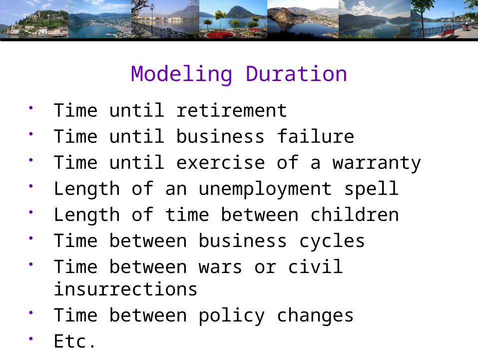
Modeling Duration

• Time until retirement• Time until business failure• Time until exercise of a warranty• Length of an unemployment spell• Length of time between children• Time between business cycles• Time between wars or civil insurrections• Time between policy changes• Etc.

The Hazard Function

For the random variable t = time until an event occurs, t 0.

f(t) = density; F(t) = cdf = Prob[time t]= S(t) = 1-F(t) = survival

Probability of an event occurring at or before time t is F(t)

A condit

ional probability: for small > 0,

h(t)= Prob(event occurs in time t to t+ | has not already occurred)

h(t)= Prob(event occurs in time t to t+ | occurs after time t)

F(t+ )-F(t) =

1 F(t)

Consider a

s 0, the function

F(t+ )-F(t) f(t)(t) =

(1 F(t)) S(t)

f(t)(t) the "hazard function" and (t) Prob[time t time+ | time t]

S(t)

(t) is a characteristic of the distribution

Hazard Function

t

0

t

0

t

0

Since (t) = f(t)/S(t) = -dlogS(t)/dt,

F(t) = 1 - exp - (s)ds ,t 0.

dF(t) / dt exp - (s)ds ( 1) (t)

(t)exp - (s)ds (Leibnitz's Theorem)

Thus, F(t) is a function of the ha

zard;

S(t) = 1 - F(t) is also,

and f(t) = S(t) (t)

A Simple Hazard Function

The Hazard function

Since f(t) = dF(t)/dt and S(t) = 1-F(t),

f(t) h(t)= =-dlogS(t)/dt

S(t)

Simplest Hazard Model - a function with no "memory"

(t) = a constant,

f(t)dlogS(t) / dt.

S(t)

The second

simplest differential equation;

dlogS(t) / dt S(t) Kexp( t), K = constant of integration

Particular solution requires S(0)=1, so K=1 and S(t)=exp(- t)

F(t) = 1-exp(- t) or f(t)= exp( t), t 0. Exponent

ial model.

Duration Dependence

When d (t)/dt 0, there is 'duration dependence'

Parametric Models of Duration

p-1

p-1 p

There is a large menu of parametric models for survival analysis:

Exponential: (t)= ,

Weibull: (t)= p( t) ; p=1 implies exponential,

Loglogistic: (t)= p( t) / [1 ( t) ],

Lognormal: (t

)= [-plog( t)]/ [-plog( t)],

Gompertz: (t)=p exp( t),

Gamma: Hazard has no closed form and must be

numerically integrated,

and so on.

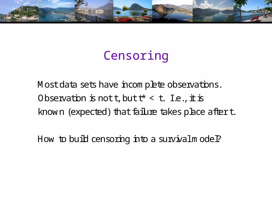
Censoring

Most data sets have incomplete observations.

Observation is not t, but t* < t. I.e., it is

known (expected) that failure takes place after t.

How to build censoring into a survival model?

Accelerated Failure Time Models

p-1

(.) becomes a function of covariates.

=a set of covariates (characteristics) observed at baseline

Typically,

(t| )=h[exp( ),t]

E.g., Weibull: (t| )=exp( )p[exp( )t]

E.g., Exponential: (t| )=ex

x

x x

x x x

x

p( )[exp( )t];

f(t| )=exp( )exp[-exp( )t]

x x

x x x

Proportional Hazards Models

p p-1

(t | ) g( ) (t)

(t) = the 'baseline hazard function'

Weibull: (t| )=pexp( ) (t)

None of Loglogistic, F, gamma, lognormal, Gompertz,

are proportional hazard models.

x x

x x

ML Estimation of Parametric Models

d (1 d)

Maximum likelihood is essentially the same as for the tobit model

f(t| ) = density

S(t| ) = survival

For observed t, combined density is

g(t| )=[f(t| )] [S(t | )]

d = 1 if not censored, 0 if censored.

x

x

x x x

d

d

n

i i i i ii 1

Rearrange

f(t| )g(t| )= [S(t | )] [ (t | )] S(t | )

S(t | )

logL d log (t | ) logS(t | )

xx x x x

x

x x

Time Varying Covariates

Hazard function must be defined as a function of

the covariate path up to time t;

(t,X(t)) = ...

Not feasible to model a continuous path of the

individual covariates. Data may be observed at

specific int

1 1 2ervals, [0,t | x(0)),[t , t | x(1)),...

Treat observations as a sequence of observations.

Build up hazard path piecewise, with time invariant

covariates in each segment. Treat each interval

save for the last as a censored (at both ends) observation.

Last observation (interval) might be censored, or not.

Unobserved Heterogeneity

Typically multiplicative -

(t| ,u)=u (t| )

Also typical:

(t| ,u)=u [exp( ), t]

In proportional hazards models like Weibull,

(t| ,u)=uexp( ) [t] exp( ) [t]

Approaches: Assume

variable with mean 1.

x x

x x

x x x

f(u), then integrate u out of f(t| ,u).

(1) (log)Normally distributed (u), amenable to quadrature

(Butler/Moffitt) or simulation based estimation

exp( u)u(2) (very typical). Log-gamma u has f(u)=

x

1

+1 P 1

P 1/

( )

[A(t)] p( t)Produces f(t| )= ,

[1 ( t) ]

A(t) = survival function without heterogeneity, for exponential or Weibull.

x

Interpretation

• What are the coefficients?• Are there ‘marginal effects?’• What quantities are of interest in

the study?

Cox’s Semiparametric Model

s k

i i i 0 i

ii k k

sAll individuals with t T

Cox Proportional Hazard Model

(t | ) exp( ) (t )

Conditional probability of exit - with K

distinct exit times in the sample:

exp( )Prob[t T | ]

exp( )

(The set of

x x

xX

x

s k individuals with t T is the risk set.

Partial likelihood - simple to maximize.

Nonparametric Approach

• Based simply on counting observations• K spells = ending times 1,…,K• dj = # spells ending at time tj

• mj = # spells censored in interval [tj , tj+1)• rj = # spells in the risk set at time tj = Σ

(dj+mj)

• Estimated hazard, h(tj) = dj/rj

• Estimated survival = Πj [1 – h(tj)] (Kaplan-Meier “product limit” estimator)

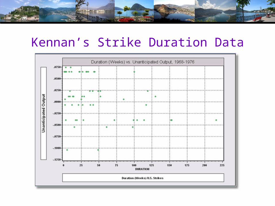
Kennan’s Strike Duration Data

Kaplan Meier Survival Function

Hazard Rates

Kaplan Meier Hazard Function

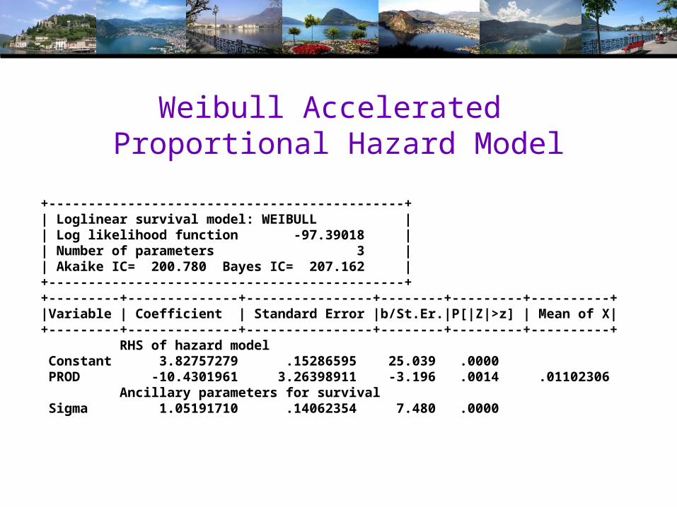
Weibull Accelerated Proportional Hazard Model

+---------------------------------------------+| Loglinear survival model: WEIBULL || Log likelihood function -97.39018 || Number of parameters 3 || Akaike IC= 200.780 Bayes IC= 207.162 |+---------------------------------------------++---------+--------------+----------------+--------+---------+----------+|Variable | Coefficient | Standard Error |b/St.Er.|P[|Z|>z] | Mean of X|+---------+--------------+----------------+--------+---------+----------+ RHS of hazard model Constant 3.82757279 .15286595 25.039 .0000 PROD -10.4301961 3.26398911 -3.196 .0014 .01102306 Ancillary parameters for survival Sigma 1.05191710 .14062354 7.480 .0000

Weibull Model

+----------------------------------------------------------------+ | Parameters of underlying density at data means: | | Parameter Estimate Std. Error Confidence Interval | | ------------------------------------------------------------ | | Lambda .02441 .00358 .0174 to .0314 | | P .95065 .12709 .7016 to 1.1997 | | Median 27.85629 4.09007 19.8398 to 35.8728 | | Percentiles of survival distribution: | | Survival .25 .50 .75 .95 | | Time 57.75 27.86 11.05 1.80 | +----------------------------------------------------------------+

Survival Function

Duration

.20

.40

.60

.80

1.00

.00

10 20 30 40 50 60 70 800

Estimated Survival Function for LO GCT

Su

rviv

al

Hazard Function with Positive Duration Dependence for All t

Duration

.0050

.0100

.0150

.0200

.0250

.0300

.0350

.0400

.0000

10 20 30 40 50 60 70 800

Estimated H azard Function for LO GCT

Ha

za

rdF

n

Loglogistic Model

+---------------------------------------------+| Loglinear survival model: LOGISTIC || Dependent variable LOGCT || Log likelihood function -97.53461 |+---------------------------------------------++---------+--------------+----------------+--------+---------+----------+|Variable | Coefficient | Standard Error |b/St.Er.|P[|Z|>z] | Mean of X|+---------+--------------+----------------+--------+---------+----------+ RHS of hazard model Constant 3.33044203 .17629909 18.891 .0000 PROD -10.2462322 3.46610670 -2.956 .0031 .01102306 Ancillary parameters for survival Sigma .78385188 .10475829 7.482 .0000+---------------------------------------------+| Loglinear survival model: WEIBULL || Log likelihood function -97.39018 ||Variable | Coefficient | Standard Error |b/St.Er.|P[|Z|>z] | Mean of X|+---------+--------------+----------------+--------+---------+----------+ RHS of hazard model Constant 3.82757279 .15286595 25.039 .0000 PROD -10.4301961 3.26398911 -3.196 .0014 .01102306 Ancillary parameters for survival Sigma 1.05191710 .14062354 7.480 .0000

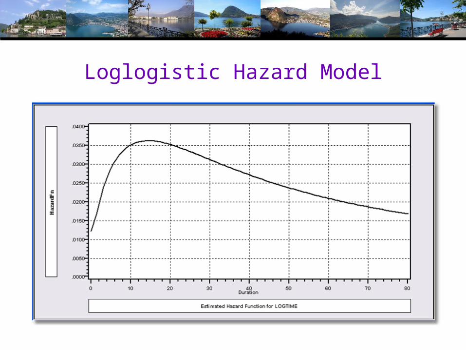
Loglogistic Hazard Model

Log Baseline Hazards

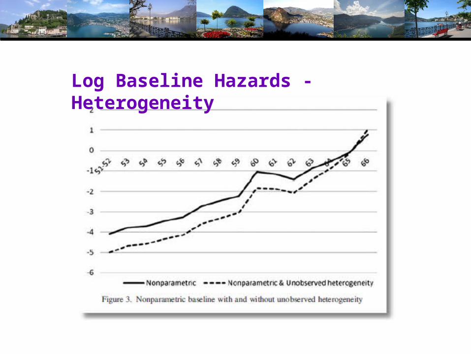
Log Baseline Hazards - Heterogeneity