165-2011: eliminating response style segments in survey...

1

Paper 165-2011

Eliminating Response Style Segments in Survey Data via Double Standardization Before Clustering

Murali Krishna Pagolu and Goutam Chakraborty, Oklahoma State University, Stillwater, OK

ABSTRACT

Segmentation is the process of dividing a market into groups so that members within the groups are very similar with respect to their needs, preferences, and behaviors but members between groups are very dissimilar. Marketers often use clustering to find segments of respondents in data collected via surveys. However, such data often exhibits response styles of respondents. For example, if some respondents use only the extreme ends of scales for answering questions in a survey, the clustering method will identify that group as a unique segment, which cannot be used for segmentation. In this paper, we first discuss the different data transformation methods that are commonly used before clustering. We then apply these different transformations to survey data collected from 959 customers of a business-to-business company. Both hierarchical and k-means clustering are then applied to the transformed data. Our results show that double-standardization performs better than other transformations in eliminating groups that identify response styles. We show how double-standardization can be achieved on any data using SAS

® programs and SAS

® macros.

INTRODUCTION

All businesses rely on customers’ continuous feedback in order to improve services or standards. To achieve this, customers’ perceptions or attitudes towards the organization are measured and assessed. This is often achieved by means of questionnaire or survey methodology, which is usually a set of questions measuring customers’ attitudes/perceptions. However, it is often difficult to record customers’ true intentions and attitudes from surveys/questionnaires due to the bias effects introduced in the data (Bachman, 1984). One of the main reasons for a bias in measuring customers’ attitudes or perceptions is the response style behavior. Response styles in questionnaire/survey data is defined as the systematic inclination of responders to answer questions based on some unknown effect other than the content of the question (Paulhus, 1991, p. 17).

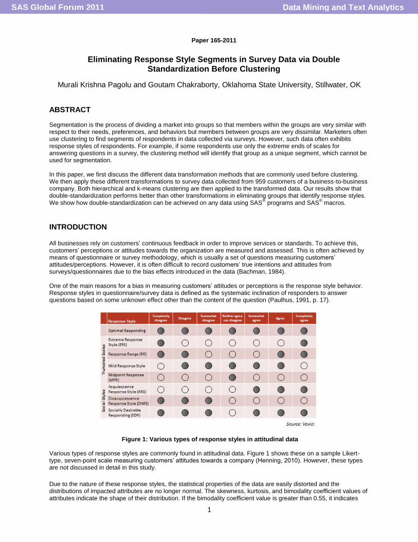
Figure 1: Various types of response styles in attitudinal data

Various types of response styles are commonly found in attitudinal data. Figure 1 shows these on a sample Likert-type, seven-point scale measuring customers’ attitudes towards a company (Henning, 2010). However, these types are not discussed in detail in this study.

Due to the nature of these response styles, the statistical properties of the data are easily distorted and the distributions of impacted attributes are no longer normal. The skewness, kurtosis, and bimodality coefficient values of attributes indicate the shape of their distribution. If the bimodality coefficient value is greater than 0.55, it indicates

Data Mining and Text AnalyticsSAS Global Forum 2011

2

that the distribution is no longer uniform and does not yield better results for clustering (Der & Everitt, p. 273, 2002). These values impact the performance of clustering procedures or any other unsupervised or supervised model in general. Various forms of standardization have been proposed and tested in last few years. However, very few of them stand out in terms of applicability and validity of data collected in diverse fields of study. Some of the key standardization forms are addressed in this paper. Standardization refers to data transformation that involves correction of scores of either attributes or cases using either means or standard deviations or both. When the adjustment to the original scores is made using means, adjusted scores are produced as the mean across attributes or cases are subtracted from the original mean of either an attribute or a case (Fischer, 2004). The resulting adjusted score is often further adjusted using standard deviation. Standardization might be based on the adjustment of means of either cases, attributes, or both using either the mean across attributes for each case or across cases within an attribute, or both (Fischer, 2004). Thus the type of standardization to adjust raw scores relies on the type of the information (e.g., cases, attributes) and the kind of information used: means, standard deviations, or both, depending on the data and context of analysis (Fischer, 2004).

RANGE STANDARDIZATION: This form of standardization is most helpful when attributes are measured on

different scales. Attributes with large values and a wide range of variation have significant effects on the final similarity measure. Hence, it is essential to make sure that each attribute is evenly constituted in the distance measurement by means of data standardization (Vickers, 2007). Range standardization is obtained by subtracting the minimum value of the attribute from each of its scores and dividing it by the range of the attribute (Maximum – Minimum). The resulting standardized data by this method produces attributes with values in the range of 0 and 1.

CENTERING: Centering refers to scores being adjusted using only the mean across the cases (Aiken & West,

1991). The attribute mean is subtracted from its original score. Standard deviation is not adjusted in this process.

NORMAL STANDARDIZATION: This form of standardization refers to correction of the scores using the attribute

mean. The attribute mean is subtracted from its original score and then divided by the standard deviation (Howell, 1997). Hence, the resulting standardized score is the relative value of one specific case on one attribute relative to the value of other cases in that attribute. The mean across all the cases is zero and, assuming a normal distribution of responses, the resulting standard deviation will be equal to 1 (Fischer, 2004).

ROW-CENTERING: Row-centering refers to adjusting the scores using the mean of a case across all attributes

(Fischer, 2004). The mean across all of the attributes for that particular case is subtracted from each individual’s original measured value. Standard deviation is not adjusted in this process.

ROW STANDARDIZATION: This transformation refers to correction of scores for each case using the mean for

that case across all attributes measured (Hofstede, 1980), which is then subtracted from each individual’s original measured value. Thus the resulting standardized score is the relative value of the case on a variable corresponding to the other scores (Hicks, 1970). Hicks (1970) coined the term “ipsatization,” which means the process of making the mean across all attributes for a case equal to zero. These newly assessed scores can be further adjusted for differences in the variation of the ratings around the mean by dividing the resulting score with the standard deviation across attributes for that case (Fischer, 2004).

DOUBLE-CENTERING: Double-centering refers to adjustments made using both the attribute mean and the mean

of individual cases across all attributes (Fischer, 2004). Again, like centering and row-centering, this process does not involve further adjustment of scores using standard deviation.

DOUBLE STANDARDIZATION: In this process, the scores are first adjusted within the case and then the

resulting scores are adjusted within the attribute (Fischer, 2004). Thus the mean for each case across attributes and the mean for each attribute across all cases will be zero. With the assumption that the raw data is normal, the correction using the standard deviation will produce standard deviations of 1 for both cases across attributes and attributes across cases. This combination of row and normal standardization was introduced by Leung and Bond (1989) and is named “Double Standardization.” However, the order of using the row and normal standardization in combination is somewhat ambiguous. It is unclear whether the attributes should be standardized before the cases are standardized or vice versa. However, if data is standardized across attributes after standardizing across cases, then the properties of attributes are likely deformed and the true form of data is not available for study (SAS Institute Inc., p.989, 2004). The most commonly used standardization procedures are row standardization and double standardization (Fischer, 2004).


3

METHODOLOGY

XYZ is a leading supplier of hydraulic and pneumatic products serving more than 50,000 customers in U.S. (The name of the company is kept anonymous for privacy reasons.) We used survey data collected from 959 customers based on their perception of important factors in selecting a supplier for the hydraulic and pneumatic products (Table 1). XYZ would like to segment their customers based on that perception. This study is focused on going through various forms of transformations for the given data and then applying hierarchical clustering and k-means procedures to find clean and stable cluster solutions feasible in the business world to segment and profile the customers. Throughout the clustering procedures performed in this study, the average linkage method is used for fair comparison across the transformed forms of data. This method is based on average similarity of all observations or cases within a cluster and is likely to produce clusters with small within-cluster variation, which is less impacted by the presence of outliers in the data.

Table 1: Important factors for customers in selecting a supplier for the hydraulic and pneumatic products

HIERARCHICAL CLUSTERING

Performing simple hierarchical clustering using the average linkage method with no data transformations on the original data set produced the results below. The summary statistics, including skewness, kurtosis, and bimodality coefficients, of all rating attribute data in the data set are displayed in the result (Figure 1.a). The mean values vary between attributes, as do the standard deviations. Few of the attributes have bimodality coefficients greater than 0.55, which indicates non-uniform distributions. Skewness and kurtosis values for a few variables are much higher, indicating nonsymmetrical distributions. Figure 1.b shows the last 10 generations of hierarchical clustering on the original data set; it is evident that few observations join the clusters very late. This shows that the original data set should not be used straight away for clustering procedures and that it definitely needs some sort of data transformation.

Figure 1.a Figure 1.b

RANGE STANDARDIZATION: Results of hierarchical clustering show no improvement in skewness, kurtosis, or

bimodality coefficient values of the rating attribute data when compared to the results from hierarchical clustering on the original data set (Figures 1.a, 2.a). Figure 2.b shows the last 10 generations of hierarchical clustering, and we can see that the observations still join the clusters very late. Hence, we see that centering has proven useless with regard to dealing with distributions of attributes or the outliers in the data.


4


CENTERING: When compared to the results from hierarchical clustering on the original data set (Figures 1.a, 3.a),

the results of hierarchical clustering using centered data show no improvement in skewness, kurtosis, or bimodality coefficient values of the rating attributes. Figure 3.b shows the last 10 generations of hierarchical clustering; we can see that the observations still join the clusters very late. Hence, we find that centering has proven useless with regard to dealing with distributions of attributes or the outliers in the data.


NORMAL STANDARDIZATION: From the results of hierarchical clustering, we see no change in skewness, kurtosis,

or bimodality coefficient values of the rating attribute data when compared to the results from hierarchical clustering on the original data set (Figures 1.a, 4.a). Figure 4.b shows the last 10 generations of hierarchical clustering; we can see the observations join clusters very late. Thus, we find that this method proves less useful with regard to dealing with distributions of attributes or the outliers in the data.


ROW-CENTERING: Based on the results of hierarchical clustering, we see significant improvement in the skewness,

kurtosis, and bimodality coefficient values of the rating attribute data when compared to the results from hierarchical clustering on the original data set and also in comparison with the normal standardized data set (Figures 1.a, 4.a, and 5.a). Figure 5.b shows the last 10 generations of hierarchical clustering; we find that the observations still join the clusters very late. Hence, we find that though row-centering has better skewness, kurtosis, and bimodality coefficient values than that of the original data and within-case standardized data, it is still not very effective in handling the outliers in the data.


5


ROW STANDARDIZATION: Based on the results of hierarchical clustering, we see significant improvement in the

skewness, kurtosis, and bimodality coefficient values of the rating attribute data when compared to the results from hierarchical clustering on the original data set (Figures 1.a, 6.a).


Figure 6.b shows the last 10 generations of hierarchical clustering; we see that the observations still join the clusters very late. Hence, we find that though within-case standardization shows a significant impact in improving the skewness, kurtosis, and bimodality coefficient values of the original data, it is not so effective in handling the outliers in the data. DOUBLE-CENTERING: Comparing the results of hierarchical clustering with that of other forms of standardized data,

we see that the skewness and kurtosis are better than most forms of transformed data. However, the bimodality coefficient values of the rating attribute data are the best among all forms of transformed data or the original data itself (Figures 1.a, 4.a, 5.a, 6.a, and 7.a). Observing the last 10 generations of the results from hierarchical clustering in Figure 7.b, we see that there are some cases that join the clusters very late in the final stages of clustering. Thus, we can infer that double-centered data helps reduce the skewness, kurtosis, and bimodality coefficient values of data compared to various other forms of transformed data.


DOUBLE STANDARDIZATION: From the results of hierarchical clustering, we see that the skewness, kurtosis, and

bimodality coefficient values of the rating attribute data are best when compared to the results from hierarchical clustering on various other forms of transformed data or the original data set itself (Figures 1.a, 4.a, 5.a, 6.a, 7.a, and 8.a).


6


Observing the last 10 generations of the results from hierarchical clustering in Figure 8.b, we see that there are no instances where single observations join the clusters late. Hence, we can conclude that the double-standardized data proves to be better than the original data or other forms of transformed data in effectively handling the skewness, kurtosis, or bimodality coefficient of the rating attribute data and outliers in the data without actually trimming down the data. Based on the local peaking of Pseudo F and Pseudo T-squared plots, the number of clusters suggested by the results of hierarchical clustering is 6 or 7 (Figure 8.c). The code in the Appendix labeled “code for creating the double standardized data and applying hierarchical clustering” shows the method for creating the required

double standardized data and applying hierarchical clustering.

Figure 8.c

K-MEANS CLUSTERING

Below are the various forms of transformed data used in k-means algorithms for the clustering procedure. The resulting output after running the k-means algorithm for each form of the transformed data using an average linkage method (until otherwise stated) is presented below.

UNTRANSFORMED DATA: When the original data is used, 5 clusters are formed but one cluster shows one

observation (See Figure 9.a). RANGE STANDARDIZED DATA: The range standardized form of survey data produced an 11-cluster solution,

which is not feasible in real-world applications and with the size of smaller clusters with respect to the overall size of the data (See Figure 9.b). CENTERED DATA: The centered form of survey data produced a 5-cluster solution and it appears worse compared

to the clusters generated by original data. Also, we still have one cluster with only one observation (See Figure 9.c). NORMAL STANDARDIZED DATA: The normal standardized form of survey data produced a 13-cluster solution,

which is not feasible in real-world applications and with the size of smaller clusters with respect to the overall size of the data (See Figure 9.d).


7

ROW-CENTERED DATA: The row centered form of survey data produced a 7-cluster solution, which is better than

clusters generated by the earlier forms of data (See Figure 9.e). ROW STANDARDIZED DATA: Using row standardized data produces a 9-cluster solution, but again with one

observation each in two of the clusters. This is not a feasible solution given the size of the smaller clusters relative to the size of the larger clusters or the overall data (See Figure 9.f). DOUBLE-CENTERED DATA: Using double-centered data produces an 8-cluster solution, but again with one

observation each in two of the clusters. This is not a feasible solution given the size of the smaller clusters relative to the size of the larger clusters or the overall data (See Figure 9.g). DOUBLE-STANDARDIZED DATA: Using double-standardization produces a 7-cluster solution where the cluster

sizes are comparable and significant in relation to the overall data. This is similar to the clusters generated from row-centered data. However, these cluster solutions appear more feasible (see Figure 9.h) as the frequency of observations in each of the clusters indicates a more stable and cleaner cluster solution than row-centered data (see Figure 9.e).

Figure 9.a Figure 9.b Figure 9.c Figure 9.d

Figure 9.e Figure 9.f Figure 9.g Figure 9.h

The segments formed by running the k-means procedure on various forms of the original data are then assessed for response styles. The code in the Appendix labeled “SAS Code nodes to compare and assess the response style impact of data on customer segments” is used to calculate the overall mean of the perception attributes in addition

to the individual segment level mean for these attributes for each form of the transformed data as shown in Figure 10.

Figure10: Overall mean and segment-wise mean of perception attributes in the original survey data Figure 11 shows the individual segment level mean and overall mean of perception attributes resulting from running the code in Appendix labeled “SAS Code nodes to compare and assess the response style impact of data on customer segments” using the double standardized data. If eight out of the ten perception attributes in a segment

show segment level means much higher or lower when compared to the overall mean, then that segment is regarded as a problematic segment still exhibiting the response styles.


8

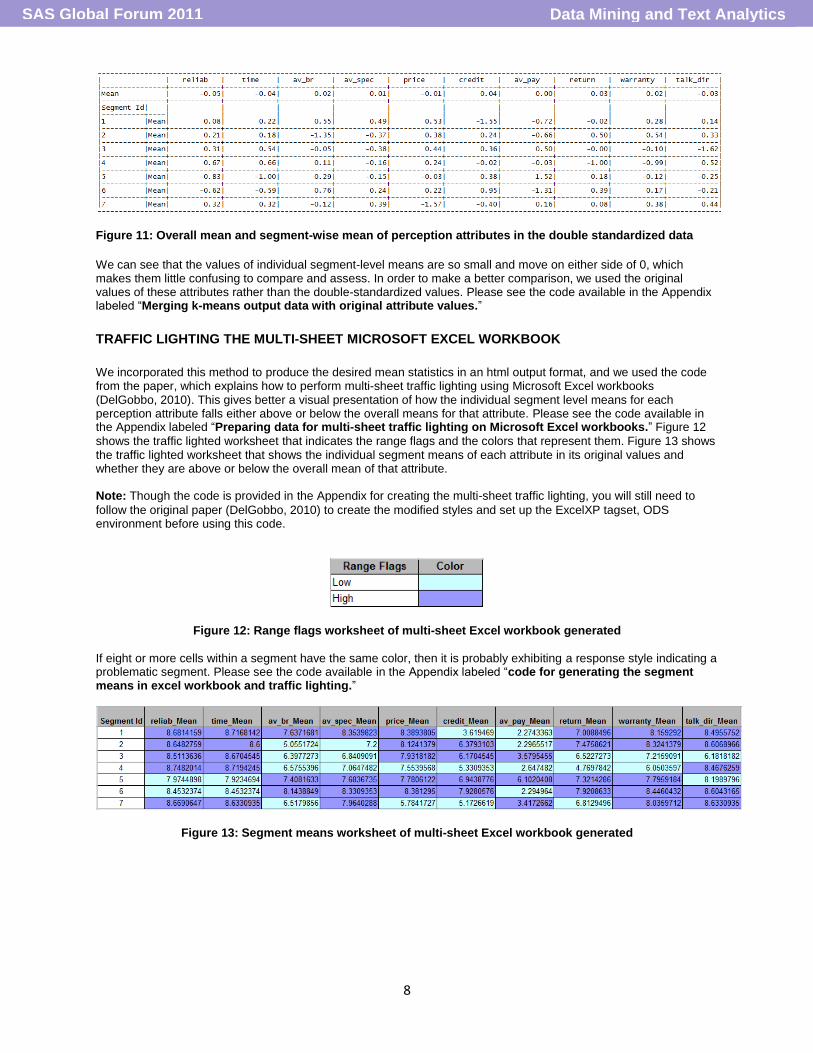
Figure 11: Overall mean and segment-wise mean of perception attributes in the double standardized data

We can see that the values of individual segment-level means are so small and move on either side of 0, which makes them little confusing to compare and assess. In order to make a better comparison, we used the original values of these attributes rather than the double-standardized values. Please see the code available in the Appendix labeled “Merging k-means output data with original attribute values.”

TRAFFIC LIGHTING THE MULTI-SHEET MICROSOFT EXCEL WORKBOOK

We incorporated this method to produce the desired mean statistics in an html output format, and we used the code from the paper, which explains how to perform multi-sheet traffic lighting using Microsoft Excel workbooks (DelGobbo, 2010). This gives better a visual presentation of how the individual segment level means for each perception attribute falls either above or below the overall means for that attribute. Please see the code available in the Appendix labeled “Preparing data for multi-sheet traffic lighting on Microsoft Excel workbooks.” Figure 12

shows the traffic lighted worksheet that indicates the range flags and the colors that represent them. Figure 13 shows the traffic lighted worksheet that shows the individual segment means of each attribute in its original values and whether they are above or below the overall mean of that attribute. Note: Though the code is provided in the Appendix for creating the multi-sheet traffic lighting, you will still need to

follow the original paper (DelGobbo, 2010) to create the modified styles and set up the ExcelXP tagset, ODS environment before using this code.

Figure 12: Range flags worksheet of multi-sheet Excel workbook generated

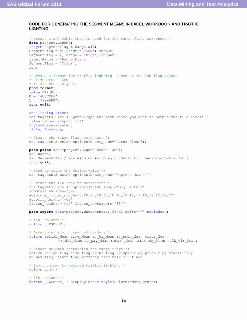
If eight or more cells within a segment have the same color, then it is probably exhibiting a response style indicating a problematic segment. Please see the code available in the Appendix labeled “code for generating the segment means in excel workbook and traffic lighting.”

Figure 13: Segment means worksheet of multi-sheet Excel workbook generated


9

RESULTS

A summary of the results from hierarchical clustering and k-means procedures are shown in a single table to allow comparison of the relative performance of these segmentation procedures on various forms of transformed data (see Figure 14).

Figure 14: Comparison table assessing relative performance of hierarchical clustering and k-means procedure on various forms of transformed data.

*For the perception attribute “Reliability,” which is impacted the most because of response styles.

**Number of observations joining very late in the cluster generations (last 10 cluster generations from cluster

history). ***

Number of possible clusters using local peaks in Pseudo F or Pseudo T-Squared and/or surge in

Normalized RMS Distance values. #Number of segments where more than 80% of attributes continue to exhibit response styles.

KEY OBSERVATIONS:

• The skewness, kurtosis, and bimodality coefficient values have significantly improved for double-standardized data.

• The number of possible outliers is zero for double-standardized data, observing the last 10 generations of cluster history from hierarchical clustering.

• The possible number of clusters is either 6 or 7 for double-standardized data, considering results from both hierarchical clustering and k-means procedures, indicating the reliability of double-standardized data in forming a stable number of clusters.

• No response style segments are found among the segments formed using the k-means procedure for double-standardized data.

CONCLUSION

Based on the descriptive statistics and results from hierarchical and k-means clustering, we see that double-standardized data performs better than any other form of transformed data (standardized or centered). The results from hierarchical clustering suggests a six or seven cluster solution (Figure 8.c), whereas k-means results suggest a seven-cluster solution (Figure 9.h) on the double-standardized data. For all other forms of transformed data, either the number of suggested clusters is unclear or the number of cases in one or more clusters formed are not reasonable. Hence, transformation of survey data using the double-standardization method helps improve the chances of getting a better (stable and clean) cluster solution that can be used for profiling customers or raters based on their perceptions where response styles and outliers are inevitable.


10

REFERENCES

Aiken, L.S., & West, S.G. (1991). Multiple regression: Testing and interpreting interactions. Newbury Park: Sage

Publications. Bachman, J.G., & O’Malley, P.M. (1984). Yea-saying, nay-saying, and going to extremes: Blackwhite differences in

response styles. Public Opinion Quarterly, 48, 491-509. DelGobbo, V. (2009). Traffic lighting your multi-sheet Microsoft Excel workbooks the easy way with SAS

®. Available

at http://support.sas.com/resources/papers/proceedings10/153-2010.pdf. Der, G., & Everitt, B.S. (2002). Handbook of statistical analyses using SAS, 2nd edn. Chapman & Hall/CRC.

Fischer, R. (2004). Standardization to account for cross-cultural response bias - A classification of score adjustment

procedures and review of research in JCCP. Journal of Cross-Cultural Psychology, 35(3), 263-282. Henning, J. (2010). Response styles confound cross-cultural comparisons. Voice of Vovici. Vovici, 23 JUL 2010.

Web. 24 Aug 2010. <http://blog.vovici.com/blog/bid/38361/Response-Styles-Confound-Cross-Cultural-Comparisons>.

Hicks, L.E. (1970). Some properties of ipsative, normative and forced-choice normative measures. Psychological

Bulletin, 74, 167-184. Hofstede, G. (1980). Culture’s consequences: International differences in work-related values. Beverly Hills, CA:

Sage. Howell, D.C. (1997). Statistical methods for psychology. Belmont, CA: Duxbury Press. Leung, K., & Bond, M.H. (1989). On the empirical identification of dimensions for cross-cultural comparisons. Journal

of Cross-Cultural Psychology, 20, 133-151. Paulhus, D. L. (1991). Measurement and control of response bias. In J.P. Robinson, P.R. Shaver, & L.S. Wrightman

(Eds.), Measures of Personality and Social Psychological Attitudes (Vol. 1). San Diego, CA: Academic Press. SAS Institute Inc. (2004). SAS/STAT

® 9.1 User’s Guide. Cary, NC: SAS Institute Inc.

Vickers, D., & Rees, P. (2007). Creating the UK national statistics 2001 output area classification. Journal of the

Royal Statistical Society Series a-Statistics in Society, 170, 379-403.

TRADEMARKS

SAS and all other SAS Institute Inc. product or service names are registered trademarks or trademarks of SAS Institute Inc. in the USA and other countries. ® indicates USA registration. Other brand and product names are trademarks of their respective companies.

ACKNOWLEDGEMENTS

Our thanks to Mr. Will Neafsey, Brand DNA and Consumer Segmentation Manager for Ford Motor Company, for suggesting the idea of this comparison in Dr. Chakraborty’s BKS course in M2009.

CONTACT INFORMATION

The authors welcome and encourage any questions, feedback, remarks, both on- and off-topic via email. Murali Krishna Pagolu, Oklahoma State University, Stillwater, OK, [email protected] Murali Krishna Pagolu is a graduate student in Management Information Systems at Spears School of Business, Oklahoma State University. Before joining the graduate program he worked as an Information Technology consultant. He is a BASE SAS

® 9 and Advanced SAS

® 9 certified professional and a certified SAS

® predictive modeler using


11

Enterprise Miner 6. He won honorable mention award in the annual Data Mining Shootout competition in a team event and student poster competition at the individual level held by M2010 annual data mining conference. Goutam Chakraborty, Oklahoma State University, Stillwater, OK, [email protected] Goutam Chakraborty is a professor of marketing and founder of SAS

® and OSU data mining certificate program at

Oklahoma State University. He has published in many journals such as Journal of Interactive Marketing, Journal of Advertising Research, Journal of Advertising, Journal of Business Research, etc. He has chaired the national conference for direct marketing educators for 2004 and 2005 and co-chaired M2007 data mining conference. He is also a Business Knowledge Series instructor for SAS

®.

APPENDIX Note: In order to ensure that identification values are retrieved correctly on to the double-standardized data set, a

macro is written to store the identification attribute values to macro variables initially. COLn (where n is the observation position number) macro variables are stored in the global macro table based on the observation position. Once the transposed data set is standardized on mean and standard deviation and again transposed to original form, the COLn values stored in the _NAME_ attribute are used for mapping the original identification attribute values using the stored macro variables.

CODE FOR CREATING THE DOUBLE STANDARDIZED DATA AND APPLYING HIERARCHICAL CLUSTERING

* create library for the data set *;

libname project '<Type in your path for the data stored here>';

* Sort the data set by identification number *;

proc sort data=project.surveydata out=project.surveydata_sorted;

by id;

run;

* create macro variables for each identification number *;

proc sql noprint;

select count(*) into :n

from project.surveydata_sorted;

%let n=&n;

%let pref=COL;

%put Total number of observations in the data set = &n;

select id label=„id‟

into :&pref.1-:&pref&n

from project.surveydata_sorted

order by id;

quit;

* Standardize columns with 0 mean and 1 standard deviation *;

proc standard data=project.surveydata_sorted mean=0 std=1

out=project.surveydata_s;

run;

* Transpose the normal standardized data *;

proc transpose data=project.surveydata_s

out=project.surveydata_st;

run;

* Standardize columns (now columns in the transposed data set) with 0 mean and 1

standard deviation *;

proc standard data=project.surveydata_st mean=0 std=1

out=project.surveydata_sts;

run;

* Transpose the double standardized data set to original form *;

proc transpose data=project.surveydata_sts

out=project.surveydata_stst;

run;


12

* Retrieve the stored identification numbers from macro variables *;

data project.smallexample_dc_final (drop=_NAME_);

length id $ 8;

set project.surveydata_stst;

id = symget(_NAME_);

label id = „id‟;

run;

*Run hierarchical clustering procedure *;

ods graphics on;

proc cluster data=project.smallexample_dc_final

method=average

simple

ccc

pseudo

outtree=project.clustreesmallexampledc(label=“cluster tree data for

project.smallexampledc”)

print=30

plots=psf

plots=pst2

plots=ccc;

var reliab time av_br av_spec price credit av_pay return warranty talk_dir;

run;

proc tree data=project.clustreesmallexampledc

out=project.treedatasmallexampledc(label=“disjoint cluster data (from

proc tree) for project.smallexampledc”)

nclusters=10;

run;

ods graphics off;

SAS CODE NODES TO COMPARE AND ASSESS THE RESPONSE STYLE IMPACT OF DATA ON CUSTOMER SEGMENTS

* Create a cross-tabulation of segments vs. average rating in each segment and overall

data *;

data &em_export_train;

set &em_import_data;

proc tabulate;

var reliab time av_br av_spec price credit av_pay return warrant talk_dir;

class _segment_;

table mean _segment_*mean,

reliab time av_br av_spec price credit av_pay return warranty talk_dir;

run;

MERGING K-MEANS OUTPUT DATA WITH ORIGINAL ATTRIBUTE VALUES

* Both the original and the transformed variables have same names in common. Hence, we

need to rename the variables with a suffix or a prefix to ensure both the transformed

and the original variables are available after the merge To avoid any issues while

merging, converting the id variable to numeric *;

data project.kmeansdsdataset_new

( rename= (reliab=reliab_ds time=time_ds av_br=av_br_ds av_spec=av_spec_ds

price=price_ds credit=credit_ds av_pay=av_pay_ds

return=return_ds warranty=warranty_ds talk_dir=talk_dir_ds) );

length num_id 8;

set project.kmeansdsdataset;

num_id = input(id, 8.);

drop id ;

rename num_id=id ;

run;


13

* Sorting the data set with untransformed variables before match merging *;

proc sort data=project.xyz_filtered out=project.xyz_filtered_sorted;

by id;

run;

* Sorting the data set which contains the Double standardized variables and their k-

means cluster memberships *;

proc sort data=project.kmeansdsdataset_new out=project.kmeansdsdataset_sorted;

by id;

run;

* Match-merging the original filtered data set with the double standardized data set

*;

data project.kmeansdsmerged;

merge project.xyz_filtered_sorted project.kmeansdsdataset_sorted;

by id;

run;

PREPARING DATA FOR MULTI-SHEET TRAFFIC LIGHTING ON MICROSOFT EXCEL WORKBOOKS

* producing the cross-tabulation of segments vs. average rating in each segment and

overall data in a data set *;

proc tabulate data=project.kmeansdsmerged out=project.dsmeanstats;

var reliab time av_br av_spec price credit av_pay return warranty talk_dir;

class _segment_;

table mean _segment_*mean,

reliab time av_br av_spec price credit av_pay return warranty talk_dir;

run;

* drop unnecessary attributes from the data set *;

data project.dsmeanstats_new;

set project.dsmeanstats (drop= _type_ _page_ _table_);

run;

* create the range flags in a new data set required for traffic lighting by comparing

the individual mean of each attribute within a segment to its overall mean.

* flag = 0 if segment level mean is less than the overall mean

* flag = 1 if segment level mean is greater than or equal to overall mean *;

data project.dsmeansstats_final

(drop=x i rename=(flag1=reliab_flag flag2=time_flag

flag3=av_br_flag flag4=av_spec_flag

flag5=price_flag flag6=credit_flag

flag7=av_pay_flag flag8=return_flag

flag9=warranty_flag flag10=talk_dir_flag));

set project.dsmeanstats_new;

array segment_means(10) reliab_mean time_mean

av_br_mean av_spec_mean

price_mean credit_mean

av_pay_mean return_mean

warranty_mean talk_dir_mean;

array compare (10) _temporary_ ;

array flag(*) flag1-flag10;

if _segment_ eq . then

do x = 1 to dim(segment_means);

compare(x) = segment_means(x);

end;

else

do i = 1 to dim(segment_means);

if segment_means{i} < compare{i} then flag{i} = 0;

else if segment_means{i} >= compare{i} then flag{i} = 1;

else flag{i}=.;

end;

if _segment_ ne .;

run;


14

CODE FOR GENERATING THE SEGMENT MEANS IN EXCEL WORKBOOK AND TRAFFIC LIGHTING

* Create a SAS table that is used for the range flags worksheet *;

data project.Legend;

length SegmentFlag 8 Range $30;

SegmentFlag = 0; Range = 'Low'; output;

SegmentFlag = 1; Range = 'High'; output;

label Range = 'Range Flags'

SegmentFlag = 'Color';

run;

* Create a format for traffic lighting, based on the lab flag values

* 0: #CCFFFF - Low

* 1: #9999FF - High *;

proc format;

value FlagFmt

0 = '#CCFFFF'

1 = '#9999FF';

run; quit;

ods listing close;

ods tagsets.ExcelXP path=<Type the path where you want to output the file here>'

file='SegmentsReport.xml'

style=XLsansPrinter;

title; footnote;

* Create the range flags worksheet *;

ods tagsets.ExcelXP options(sheet_name='Range Flags');

proc print data=project.Legend noobs label;

var Range;

var SegmentFlag / style(column)=[foreground=FlagFmt. background=FlagFmt.];

run; quit;

* Need to reset the option value *;

ods tagsets.ExcelXP options(sheet_name='Segment Means');

* Create the lab results worksheets *;

ods tagsets.ExcelXP options(sheet_label='Big Picture'

suppress_bylines='yes'

absolute_column_width='8,10,10,10,10,10,10,10,10,12,10,12,12,12,12'

autofit_height='yes'

frozen_headers='yes' frozen_rowheaders='11');

proc report data=project.dsmeansstats_final split='*' nowindows;

* 'ID' columns *;

column _SEGMENT_;

* Data columns with spanned headers *;

column reliab_Mean time_Mean av_br_Mean av_spec_Mean price_Mean

credit_Mean av_pay_Mean return_Mean warranty_Mean talk_dir_Mean;

* Hidden columns containing the range flags *;

column reliab_flag time_flag av_br_flag av_spec_flag price_flag credit_flag

av_pay_flag return_flag warranty_flag talk_dir_flag;

* Dummy column to perform traffic lighting *;

column dummy;

* 'ID' columns *;

define _SEGMENT_ / display order style(Column)=data_center;


15

* Data columns *;

define reliab_Mean / display;

define time_Mean / display;

define av_br_Mean / display;

define av_spec_Mean / display;

define price_Mean / display;

define credit_Mean / display;

define av_pay_Mean / display;

define return_Mean / display;

define warranty_Mean / display;

define talk_dir_Mean / display;

* Hidden columns containing the range flags *;

define reliab_flag / display noprint;

define time_flag / display noprint;

define av_br_flag / display noprint;

define av_spec_flag / display noprint;

define price_flag / display noprint;

define credit_flag / display noprint;

define av_pay_flag / display noprint;

define return_flag / display noprint;

define warranty_flag / display noprint;

define talk_dir_flag / display noprint;

* Dummy column to perform traffic lighting *;

define dummy / computed noprint;

* Traffic light the data columns based on the hidden columns *;

compute dummy;

array name(10) $31 ('reliab_Mean' 'time_Mean' 'av_br_Mean' 'av_spec_Mean' 'price_Mean'

'credit_Mean' 'av_pay_Mean' 'return_Mean' 'warranty_Mean'

'talk_dir_Mean');

array flag(10) reliab_flag time_flag av_br_flag av_spec_flag price_flag credit_flag

av_pay_flag return_flag warranty_flag talk_dir_flag;

* Loop over all the _Result columns ('name' array), and set the BACKGROUND style

attribute based on the value of the corresponding _Flag column ('flag' array) *;

do i = 1 to dim(name);

if (flag(i) ge 0) then call define(name(i),'style',

'style=[background=' || put(flag(i), FlagFmt.) || ']');

end;

endcomp;

run; quit;

ods tagsets.ExcelXP close;


165-2011: eliminating response style segments in survey...

Documents