16. Tobit and SelectionA. Colin Cameron Pravin K. Trivedi

Copyright 2006

These slides were prepared in 1999.They cover material similar to Sections 16.2-16.3 and 16.5 of our subsequent bookMicroeconometrics: Methods and Applica-tions, Cambridge University Press, 2005.

INTRODUCTION

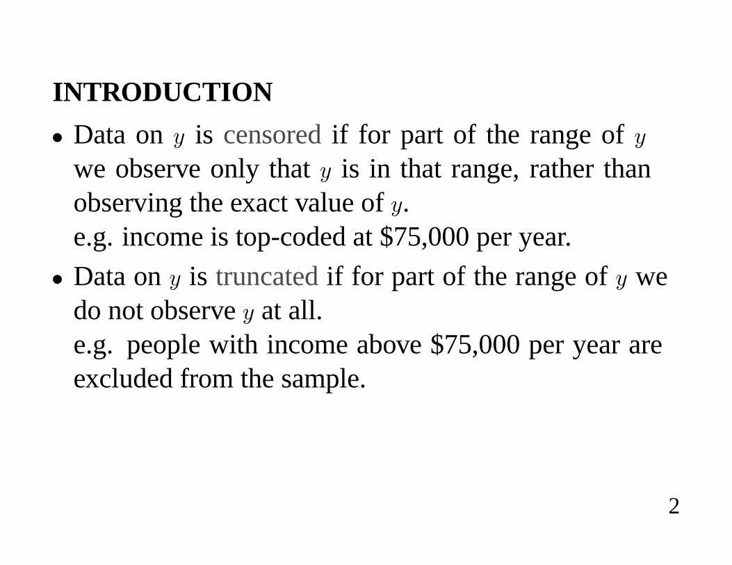
� Data on + is censored if for part of the range of +

we observe only that + is in that range, rather thanobserving the exact value of +.e.g. income is top-coded at $75,000 per year.

� Data on+ is truncatedif for part of the range of+ wedo not observe+ at all.e.g. people with income above $75,000 per year areexcluded from the sample.

2

� Meaningful policy analysis requires extrapolation fromthe restricted sample to the population as a whole.

� But running regressions on censored or truncated data,without controlling for censoring or truncation, leadsto inconsistent parameter estimates.

3

� We focus on the normal, with censoring or truncationat zero.e.g. annual hours worked, and annual expenditure onautomobiles.

� The class of models presented in this chapter is calledlimited dependent variable models or latent variablemodels. Econometricians also use the terminologytobit models or generalized tobit models.

4

� Censoring can arise for distributions other than thenormal.

� For e.g. count data treatment is similar to here exceptdifferent distributions.

� For duration data, e.g. the length of a spell of unem-ployment, aseparate treatment of censoringis giventhere due to different censoring mechanism (random)to that considered here.

5

OUTLINE

� Tobit model: MLE, NLS and Heckman 2-step.

� Sample selectivity model, a generalization of Tobit.

� Semiparametric estimation.

� Structural economic models for censored choice.

� Simultaneous equation models.

6

TOBIT MODEL

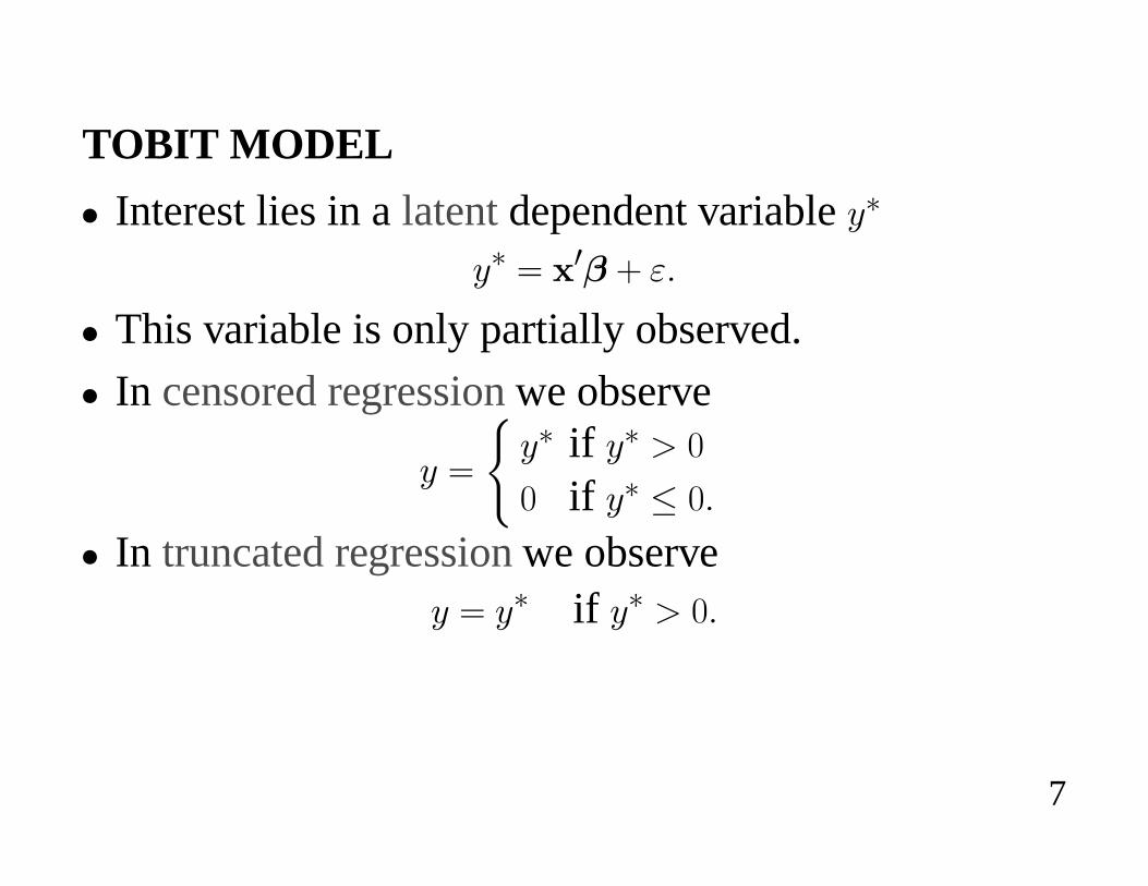
� Interest lies in a latent dependent variable +�

+� ' 3� n 0�

� This variable is only partially observed.

� In censored regression we observe

+ '

++� if +� : f

f if +� � f�

� In truncated regression we observe+ ' +� if +� : f�

7

� The standard estimators require stochastic assumptionsabout the distribution of 0 and hence +�.

� The Tobit model assumes normality:0 � 1dfc j2o , +� � 1d 3�c j2o�

8

SIMULATION EXAMPLE

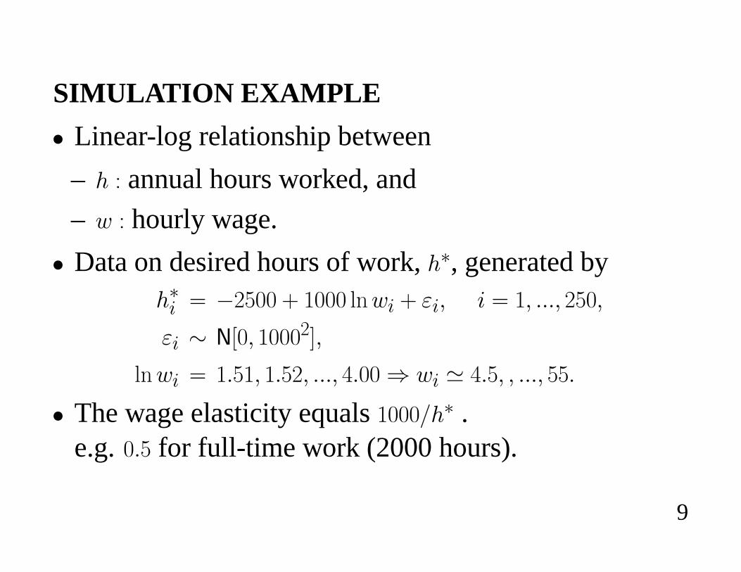
� Linear-log relationship between

– � G annual hours worked, and

– � G hourly wage.

� Data on desired hours of work,��, generated by��� ' �2Dff n �fff *?�� n 0�c � ' �c ���c 2Dfc

0� � 1dfc �fff2oc

*?�� ' ��D�c ��D2c ���c e�ff , �� * e�Dc c ���c DD�

� The wage elasticity equals�fff*�� .e.g.f�D for full-time work (2000 hours).

9

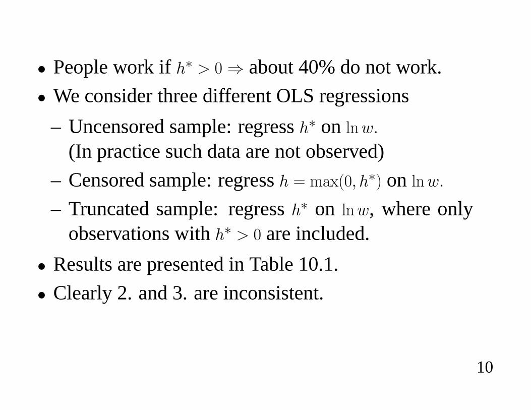
� People work if �� : f , about 40% do not work.

� We consider three different OLS regressions

– Uncensored sample: regress�� on *?��

(In practice such data are not observed)

– Censored sample: regress� ' 4@ Efc ��� on *?��

– Truncated sample: regress�� on *?�, where onlyobservations with�� : f are included.

� Results are presented in Table 10.1.

� Clearly 2. and 3. are inconsistent.

10

Variable SampleUncensored Censored Truncated

ONE -2636 -982 -382(256) (174) (297)

lnw 1043 587 477(90) (61) (95)

R2 .35 .27 .15Observations 250 250 148

11

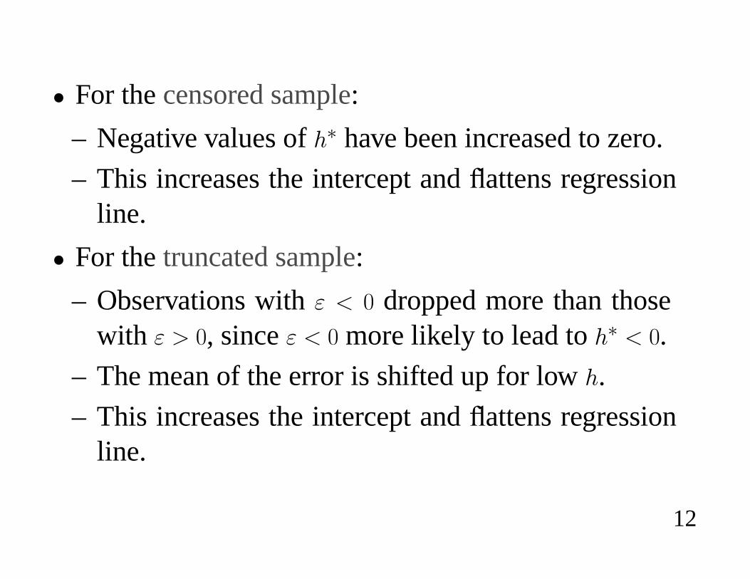
� For the censored sample:

– Negative values of�� have been increased to zero.

– This increases the intercept andÀattens regressionline.

� For thetruncated sample:

– Observations with0 f dropped more than thosewith 0 : f, since0 f more likely to lead to�� f.

– The mean of the error is shifted up for low�.

– This increases the intercept andÀattens regressionline.

12

� For censored and truncated data, linear regression isinappropriate.

13

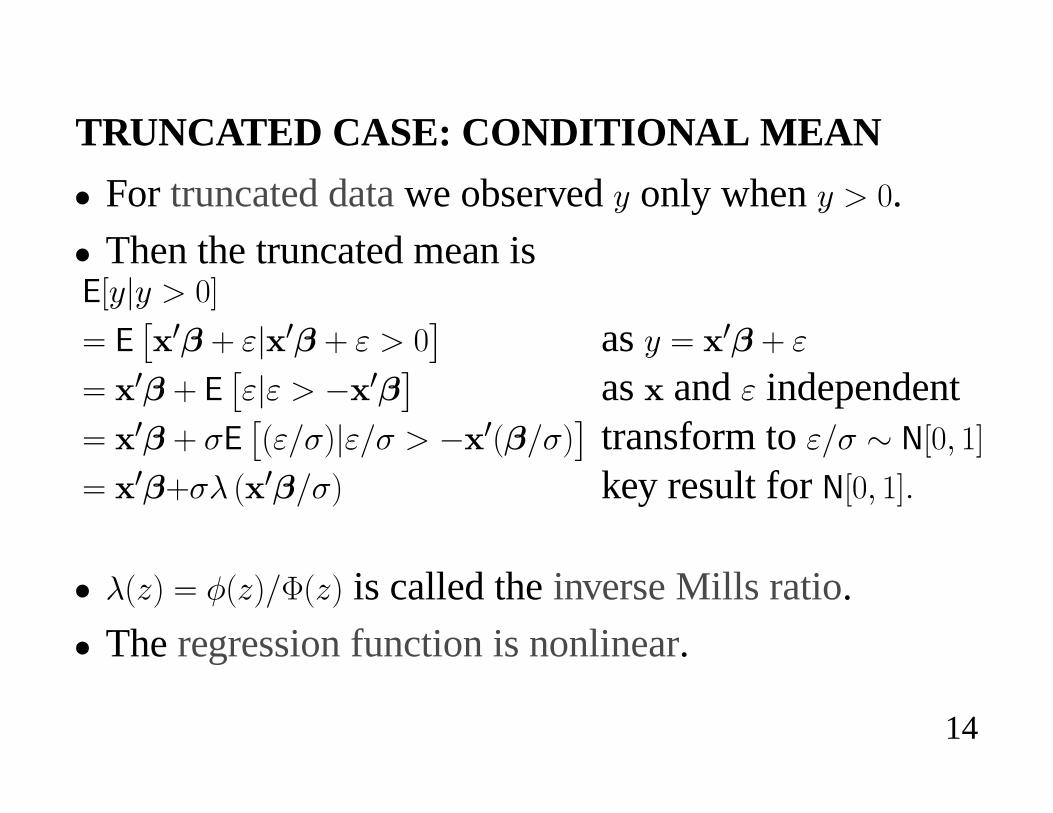
TRUNCATED CASE: CONDITIONAL MEAN

� For truncated data we observed + only when + : f.

� Then the truncated mean is(d+m+ : fo

' (� 3� n 0m 3� n 0 : f

�as + ' 3� n 0

' 3� n (�0m0 : � 3�� as and 0 independent

' 3� n j(�E0*j�m0*j : � 3E�*j�� transform to 0*j � 1dfc �o

' 3�njb E 3�*j� key result for 1dfc �o�

� bE5� ' �E5�*xE5� is called the inverse Mills ratio.

� The regression function is nonlinear.

14

� For consistent estimates use NLS or MLE, not OLS.

15

ASIDE: INVERSE MILLS RATIO

� Consider 5 � 1dfc �o, with density �E5� and cdf xE5�.

� The conditional density of 5m5 : S is �E5�*E�� x ES��.

� The truncated conditional mean is(d5m5 : So '

] 4

S5 E� E5�*E� � x ES��� _5

'

] 4

S5 �s

2Zi TE��

252� _5

!E� � x ES��

'k� �s

2Zi TE��

252�l4S

1E� � x ES��

'� ES�

�� x ES�'

� E�S�

x E�S�' bES��

16

CENSORED CASE: CONDITIONAL MEAN

� For censored data we observe + ' f if +� f and+ ' +�otherwise.

� The censored sample mean is(d+o ' (+�d(d+m+�oo

' �hd+� � fo� f n �hd+� : fo� (d+�m+� : fo

' xE 3��� 3� n j

� E 3�*j�x E 3�*j�

�' xE 3�� 3�nj� E 3�*j�c

which is again nonlinear.

� For consistent estimates use NLS or MLE, not OLS.

17

MLE FOR CENSORED DATA

� Let +� have density s�E+�� and c.d.f. 8 E+��.� Consider censored + ' 4@ E+�c f�.� The density for + is

– + : f: + ' +� sosE+� ' s�E+�.– + ' f: +� � f sosEf� ' �hd+� � fo ' 8 �Ef�.

� De¿neindicator

_ '

+� if + : f

f if + ' f�

18

� The density is thensE+� ' s�E+�_ � 8 �Ef���_�

� The log-likelihood function is

*? / '?[�'�

i_� *? s�E+�� c �c�� n E�� _�� *?8�Efc �c��j

� This is amixture of discrete and continuous densities.

19

CENSORED MLE FOR NORMAL

� For normal regression for notational convenience wetransform from sE+� the Nd 3�c j2o density to �E5� theNdfc �o density.

� For + : f

sE+� ' s�E+�'

��*s

2Zj2�� i T

��E+ � 3� �2*2j 2

�'

�

j��E+ � 3��*j

�c

where �E5� '��*s2Z

�i T

��52*2�

is Ndfc �o density.

20

� For + ' f

sEf� ' �hd+ ' fo

' �hd+� � fo

' �hd 3� n 0 � fo

' �hd0*j � � 3�*jo' x

�� 3�*j� cwhere xE5� is Ndfc �o c.d.f.

� Thus

sE+� '

��

j��E+ � 3��*�

��_ � �xE� 3�*�����_

�

21

� The log-likelihood function

*?uE�c�2� '?[�'�

+_� *?

�

j�

#+� � 3��

j

$n E�� _�� *? x

�� 3��*j�,�

22

ASYMPTOTIC THEORY

� Tobin (1958) proposed the Tobit MLE.

� He asserted that usual ML theory applied, despite thestrange continuous/discrete hybrid density.

� Amemiya (1973) provided a formal proof that usualML theory applies, with appendix that detailed theextremum estimation approach that is now standard ineconometrics.

23

� If density is correctly speci¿ed the usual ML theoryyields after some algebra% e�0/ej20/

&@� 1

57%�

j2

&c

%S@� �

3�

SK�

3�S

K� 3�

SS�

&��68 c

where de¿ning � ' �*j, �� ' �E 3��� and x� ' xE 3���,

@� ' � �

j 2 3����� n

�2��� x�

� x�

K� ' � �

j 2E 3���2 � �� n �� �

3��� �2��� x�

S� ' � �

j 2E 3���� � �� n 3��� �� �

3��� �2��� x�

2x��

24

MLE FOR TRUNCATED DATA

� For truncated data only +� : f observed.

� The conditional density iss�E+�m+� : f� ' s�E+��*�hd+�m+� : fo

' s�E+��*8 �Ef��� The log-likelihood is then

*? / '?[�'�

i*? s�E+�� c �c��� *?8 �Efc �c��j �

25

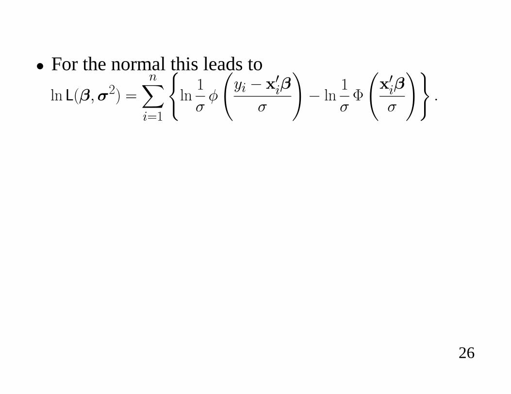
� For the normal this leads to

*? /E�c�2� '?[�'�

+*?

�

j�

#+� � 3��

j

$� *?

�

jx

# 3��j

$,�

26

NLS

� Estimate using the correct censored or truncated mean.

� Recall the censored and truncated means(d+m+ : fo ' 3�njbE 3�*��(d+o ' 3��x E 3�*j� n j� E 3�*j�c + : f

� Do NLS on these, where also control for heteroskedas-ticity as9d+m+ : fo 9' j2 and9d+o 9' j2.

� Consistency requires the nonlinear functions(d+m+ : fo

or (d+o are correctly speci¿ed.

27

� This requires strong distributional assumptions onunderlying +�.

� Any departure leads to different conditional mean func-tions and hence inconsistency of the NLS estimators.e.g. a heteroskedastic error rather than a homoskedasticerror.

� Similarly for the MLE.

� This lack of robustness has led to much research.

28

HECKMAN TWO-STEP ESTIMATOR

� Heckman (1976, 1979) proposed estimation of thecensored normal regression model by a 2-step methodrather than NLS.

� Recall from that for positive+(d+m+ : fo ' 3� n jb

�� 3�*j� cwherebE5� ' �E5�*xE5� is the inverse Mills ratio.

� Heckman noted that inconsistency of OLS of+ on isdue toomission of the regressorbE� 3�*j�.

� He proposed includingebE� 3�*j� as a regressor.

29

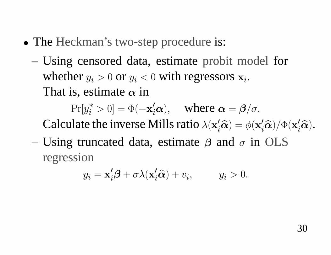
� The Heckman’s two-step procedureis:

– Using censored data, estimateprobit modelforwhether+� : f or +� f with regressors �.That is, estimate� in

�hd+�� : fo ' xE� 3���c where� ' �*j�

Calculate the inverse Mills ratiobE 3�e�� ' �E 3�e��*xE 3�e��.

– Using truncated data, estimate� and j in OLSregression

+� ' 3�� n jbE 3�e�� n ��c +� : f�

30

� Advantages:

– Consistent estimates using only probit and OLS.

– Generalizes to permit weaker assumptions.

� Disadvantages:

– Usual OLS reported standard errors are incorrect.

– Formulae for correct standard errors take account oftwo complications in the OLS regression:

– 1. Even with� known the error is heteroskedastic.

– 2. Two-step estimator with� replaced by an estimate.

– These corrections are complex.

31

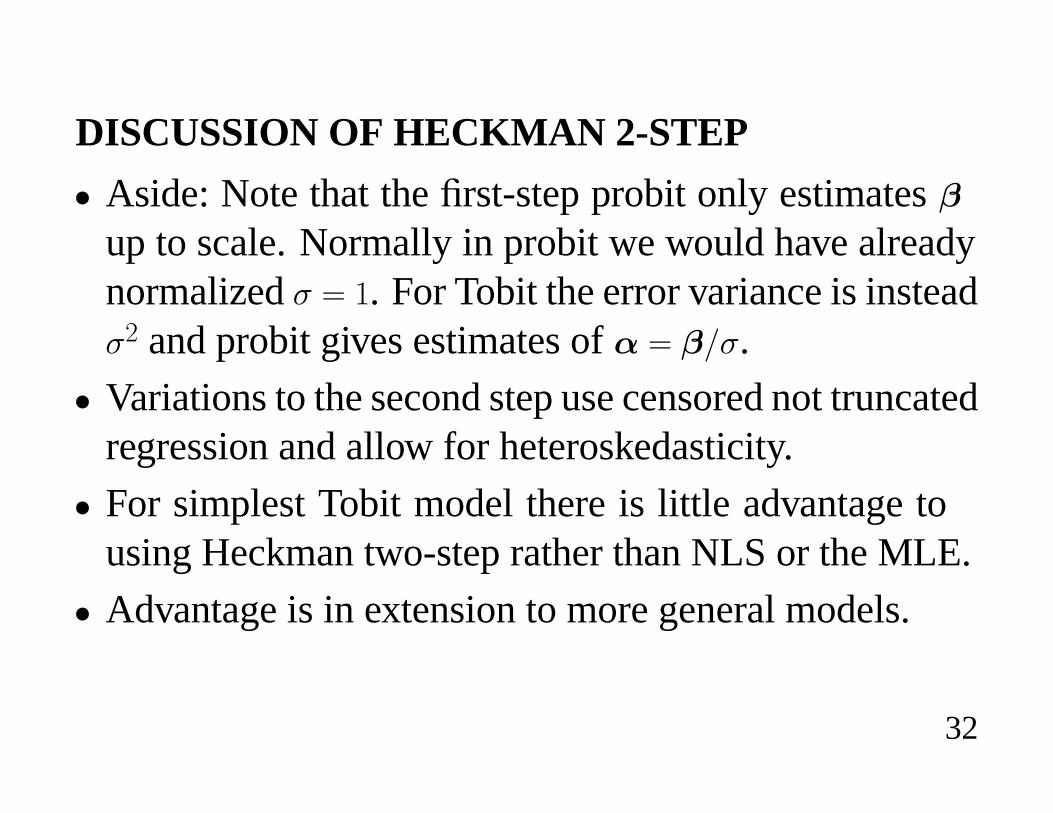
DISCUSSION OF HECKMAN 2-STEP

� Aside: Note that the ¿rst-step probit only estimates�up to scale. Normally in probit we would have alreadynormalizedj ' �. For Tobit the error variance is insteadj2 and probit gives estimates of� ' �*j.

� Variations to the second step use censored not truncatedregression and allow for heteroskedasticity.

� For simplest Tobit model there is little advantage tousing Heckman two-step rather than NLS or the MLE.

� Advantage is in extension to more general models.

32

COEFFICIENT INTERPRETATION

� Interested in how the conditional mean of dependentvariable changes as the regressors change.

� This varies according to whether we consider theuncensored mean, censored mean or truncated mean.

� Thus for hours worked consider effect of a change in aregressor on

– desired hours of work,

– actual hours of work for workers and nonworkers

– actual hours of work for workers.

33

� For the standard tobit model we obtain

� For uncensored mean(d+�m o ' 3�

Y(d+�m o*Y ' �

� For censored mean (+ ' 4@ Efc +��)(d+m o ' xE 3��i 3� n jbE 3��j

Y(d+m o*Y ' xE 3���

� For truncated mean(only + : f)(d+m o ' 3� n jbE 3��

Y(d+m o*Y ' i�� E 3��bE 3��� bE 3��2j�

34

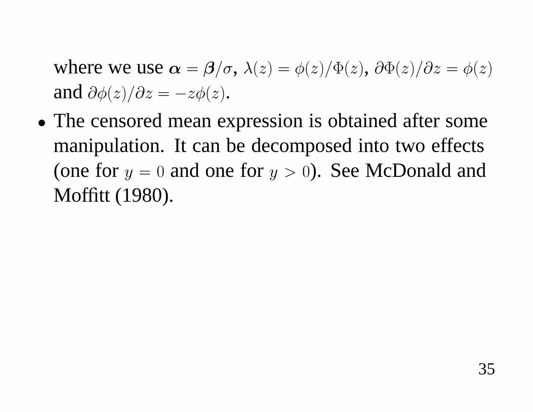
where we use � ' �*j, bE5� ' �E5�*xE5�, YxE5�*Y5 ' �E5�

and Y�E5�*Y5 ' �5�E5�.

� The censored mean expression is obtained after somemanipulation. It can be decomposed into two effects(one for + ' f and one for + : f). See McDonald andMof¿tt (1980).

35

SAMPLE SELECTIVITY MODEL

� Most common generalization of the standard tobitmodel is the sample selection or self-selectionmodel.

� This is atwo-part model

– 1. A latent variable+�� that determines whether or notthe process of interest is fully observed.

– 2. A latent variable+�2 that is of intrinsic interst.

� Classic example is labor supply

– +�� determines whether or not to work and

– +�2 determines hours of work.

36

� Complication arises as the unobserved components ofthese two processes are correlated (after controlling forregressors).

37

� The two latent variables are determined as follows+�� ' 3��� n 0�

+�2 ' 32�2 n 02c

� Neither +�� nor +�2 are completely observed.

� Instead we observe whether +�� is positive or negative

+� '

+� if +�� : f

f if +�� � f�

and only positive values of +�2

+2 '

++�2 if +�� : f

f if +�� � f�

38

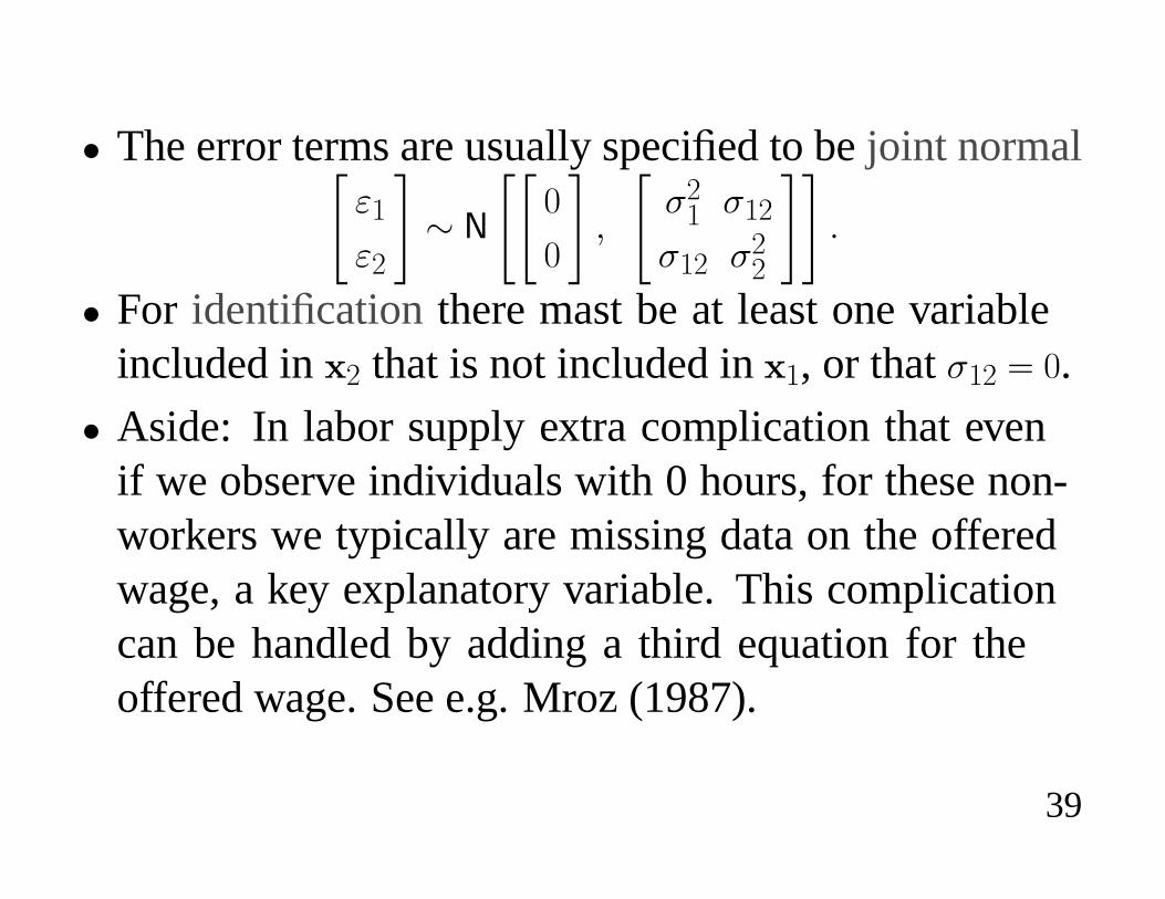
� The error terms are usually speci¿ed to be joint normal%0�

02

&� 1

%%f

f

&c

%j2� j�2

j�2 j22

&&�

� For identi¿cation there mast be at least one variableincluded in 2 that is not included in �, or that j�2 ' f.

� Aside: In labor supply extra complication that evenif we observe individuals with 0 hours, for these non-workers we typically are missing data on the offeredwage, a key explanatory variable. This complicationcan be handled by adding a third equation for theoffered wage. See e.g. Mroz (1987).

39

MLE IN SAMPLE SELECTIVITY MODEL

� The MLE maximizes the log-likelihood function.

� This is based on the joint densitysE+� c +2� ' sE+2 m+��sE+��.– The densitysE+2 m+� ' �� ' s�E+2 m+�� : f� by de¿nition.

ThussE�c +2� ' s�E+2 m+�� : f�� �hd+��: fo

– The densitysE+2 m+� ' f� places probability� on thevalue+2 ' f and probabilityf on any other value since+2 always equalsf when+� ' �.ThussEfc +2� � ' sE+2 m+� ' f�sE+� ' f� ' �hd+�� � fo.

40

� The likelihood function is

/ '?\�'�

i�hd+��� � foj��+�� �i sE+2� m +��� : f�� �hd+���: foj+�� c

� When the bivariate density is normal, the conditionaldensity in the second term is univariate normal and theproblem is not too intractable.

41

HECKMAN 2-STEP: JONT NORMALITY

� Most studies use Heckman’s method rather than ML.

� If the errorsE0�c 02� in are joint normal then02 '

j�2j2�

0� n �c

where� is independent of0�.

42

� Aside: This follows from the more general result thatfor %

3�

32

&� 1

%%��

�2

&c

%P�� P�2

P2� P22

&&the conditional distribution is32m3� � 1

k�2 n P2�P

���� E3� ����cP22 � P2�P

���� P�2

l�

� Thus 32 ' �� n P2�P���� E3� ����

plus a zero mean normal error independent of 3�.

43

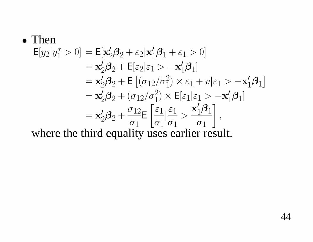
� Then(d+2m+�� : fo ' (d 32�2 n 02m 3��� n 0� : fo

' 32�2 n (d02m0� : � 3���o

' 32�2 n (�Ej�2*j

2��� 0� n �m0� : � 3���

�' 32�2 n Ej�2*j

2��� (d0�m0� : � 3���o

' 32�2 nj�2j�

(

�0�j�

m0�j�

: 3���

j�

�c

where the third equality uses earlier result.

44

� This leads to the key result that(d+2m+�� : fo ' 32�2 n

j�2j�

� b� 3����*j�

�c

where bES� ' �ES�*xES� using earlier result.

� Clearly OLS of +2 on 2 will lead to an inconsistentestimate of � since the regressor bE 3���*j��, is omittedfrom the equation.

� Heckman’s solution is to obtain an estimate of thisomitted term, and include it in the OLS regression.

45

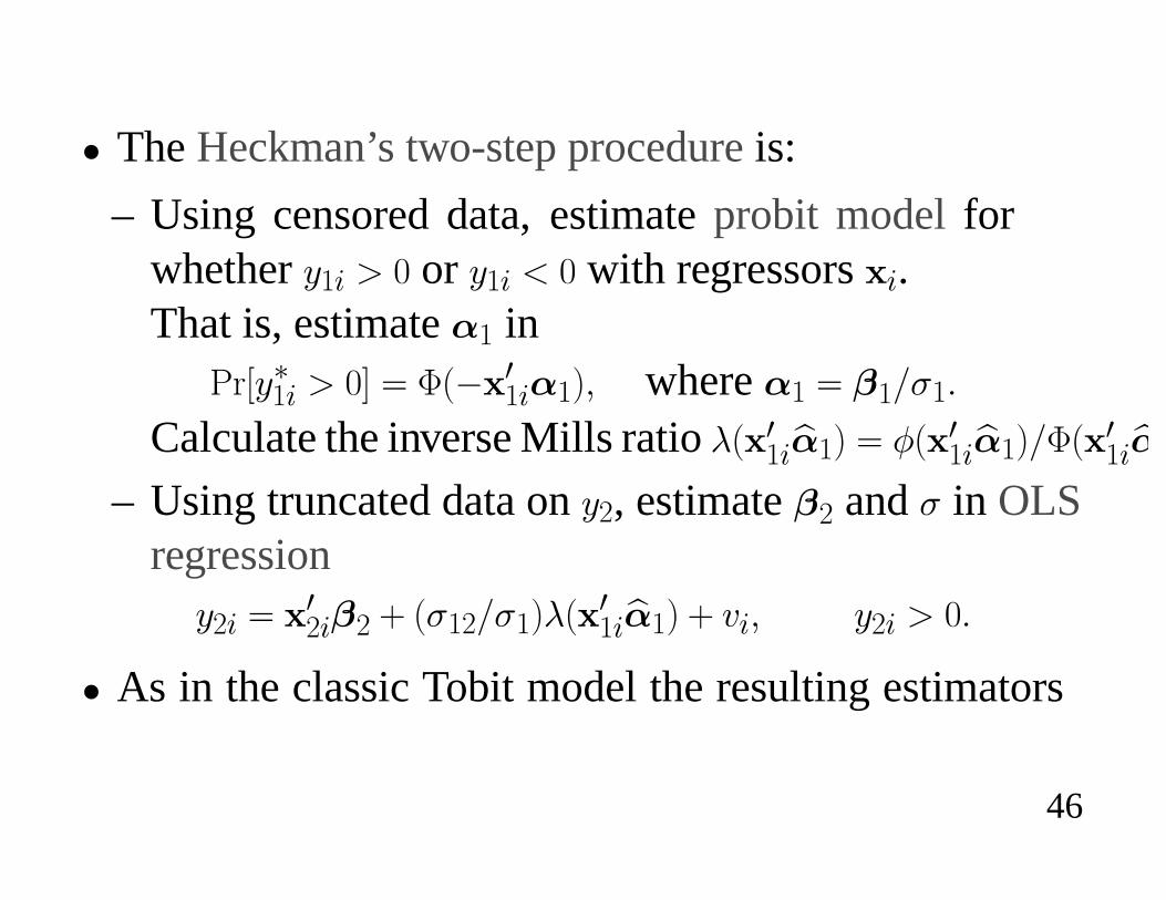
� The Heckman’s two-step procedureis:

– Using censored data, estimateprobit modelforwhether+�� : f or +�� f with regressors �.That is, estimate�� in

�hd+��� : fo ' xE� 3�����c where�� ' ��*j��

Calculate the inverse Mills ratiobE 3��e��� ' �E 3��e���*xE 3��e�

– Using truncated data on+2, estimate�2 andj in OLSregression

+2� ' 32��2 n Ej�2*j��bE 3��e��� n ��c +2� : f�

� As in the classic Tobit model the resulting estimators

46

of �2 are consistent, inef¿cient and it is cumbersome toconstruct the variance covariance matrix of OLS.

47

HECKMAN 2-STEP: WEAKER ASSUMPTIONS

� The Heckman two-step method relies onweaker distri-butional assumptionsthan the MLE.

� The MLE requires joint normality of0� and02.

� The Heckman 2-step estimator requires the weakerassumption that

02 ' B0� n �c

where� is independent of0� and0� is normally dis-tributed.

� In the case of purchase of a durable good, this says

48

that the error in the amount purhased equation is amultiple of the error in the purchase decision equation,plus some noise where the noise is independent of thepurchase decision.

� Given this assumption we obtain(d+2m+�� : fo ' 32�2 n B(d0�m0� : � 3���o�

� Heckman’s two-step method can be adapted to

– distributions for0� other than normal

– semiparametric methods which do not impose afunctional form for(d0�m0� : � 3���o.

49

COEFFICIENT INTERPRETATION

� Again interested in how the conditional mean ofdependent variable changes as the regressors change.

� This varies according to whether we consider theuncensored mean, censored mean or truncated mean.

50

� For uncensored mean(d+�2 m o ' 32�2

Y.d+�2 m 2o*Y 2 ' �2

� For censored mean(d+2m+�� : fc o ' 3�2 n Ej�2*j

2��bE

3��*j��o

Y(d+2m+�� : fc o*Y ' E��*j���E 3���*j��d

3�2 n Ej�2*j2��bE

3��*j�

nxE 3��*j��d�2 n Ej�2*j2��YbE

3��*j��*Y o

� For truncated mean...(d+2m+�� : fc o ' 3�2 n Ej�2*j

2��bE

3��*j��

Y(d+2m+�� : fc o*Y ' nEj�2*j2��YbE

3��*j��*Y o�

51

SEMIPARAMETRIC ESTIMATION

� Consistency of all the above estimators requires correctspeci¿cation of the error distribution.

� Any misspeci¿cation of the error distribution leads toinconsistency e.g. failure of normality.

� So preferable to have an estimator that does not requirespeci¿cation of the distribution of the error.

� A number of semiparametric estimators that do notrequire distribution of the error distribution have beenproposed.

52

� For the standard tobit model this has been done.

� Unfortunately, this model is often too simple and thegeneralized tobit model needs to be used. Then thereare fewer results on semiparametric estimators.

� A recent application for the sample selectivity model isgiven in Newey, Powell and Walker (1990).

� This is a major area of current research by theoreticaleconometricians.

� These often use Heckman’s two-step framework.

53

MIXED DISCRETE/CONTINUOUS MODELS

� Hanemann (1984) and Dubin and McFadden (1984)develop models from economic theory of utility maxi-mization.

54

SIMULTANEOUS EQUATIONS TOBIT MODELS

� An example is the generalized tobit model, with latentvariables

+�� ' 3��� n k�+�2 n ��+2 n 0�

+�2 ' 32�2 n k2+�� n �2+� n 02

� This has the added complication that regressors in the¿rst equation include +�2 or +2 and similarly +� or +�� inthe second equation. Identi¿cation conditions will ofcourse not permit all of these variables to be included.

� Treatment of simultaneity in these models is verydif¿cult.

55

� Often very ingenious methods allow estimation usingjust regular probit, tobit and OLS commands.

� But getting the associated standard errors of estimatorsis very dif¿cult.

� The simplest model has as right-hand side endogenousvariables only the latent variables+�2 or +��.

� We can then obtain a reduced form for+�� and+�2, inexactly the same way as regular linear simultaneousequations, and do tobit estimation on this reducedform.

� Estimators for this case are given in Nelson and Olson

56

(1978), Amemiya (1979), and Lee (1981).

� Treatment is much more dif¿cult when right-hand sideendogenous variables are the observed variables+2 or+�.

� See Heckman (1978) and Blundell and Smith (1989).

� Simultaneity in tobit (and probit) models can generallybe handled, but can require a considerable degree ofeconometric sophistication.

� If possible, specify the models such that the simultane-ity is due to the latent variables and not the observedvariables.

57

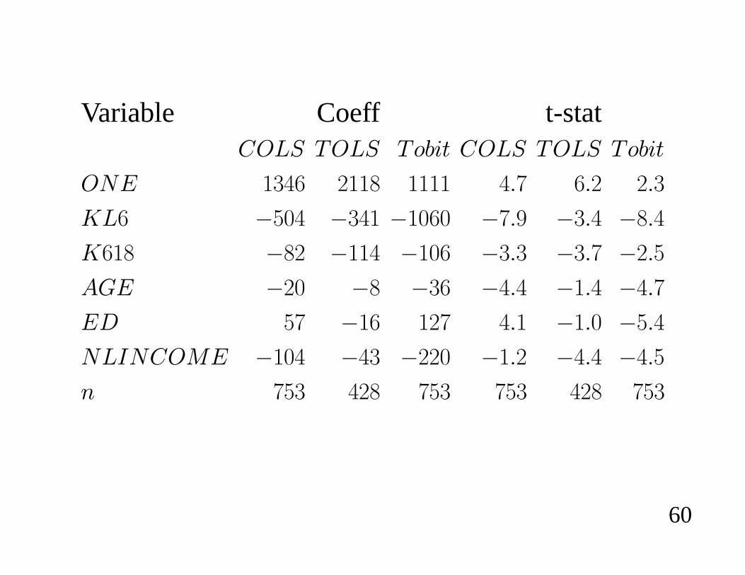
APPLICATION: LABOR SUPPLY� Use data of Mroz (1987) on 753 married women from

the 1976 Panel Survey of Income Dynamics (PSID).

� Dependent variable HOURS is annual hours worked inprevious year. For this sample there is a bunching orcensoring at zero since 225 (or 43%) had zero hours.

58

� The regressors are a constant term and

1. KL6: Number of children less than six2. K618: Number of children more than six3. AGE: Age4. ED: Education (years of schooling completed)5. NLINCOME: annual nonlabor income of wife mea-sured in $10,000’s.

59

Variable Coeff t-stat��u7 A�u7 AJK�| ��u7 A�u7 AJK�|

��. ��eS 2��H ���� e�. S�2 2��

guS �Dfe ��e� ��fSf �.�b ���e �H�e

gS�H �H2 ���e ��fS ���� ���. �2�D

�C. �2f �H ��S �e�e ���e �e�.

.( D. ��S �2. e�� ���f �D�e

�uU����. ��fe �e� �22f ���2 �e�e �e�D

? .D� e2H .D� .D� e2H .D�

60

� Estimates from censored OLS (COLS), truncated OLS(TOLS) and censored tobit (tobit) with associatedt-ratios are presented in the table.

� As observed earlier, both censoring and truncationÀatten the slope coef¿cients.

� The truncated regression suggests that some variablessuch as AGE, ED and NLINCOME may have moreimpact on the decision whether to work or not than anactual hours of work.

61

ASYMPTOTIC THEORY FOR HECKMANS’S 2-STEP METHOD

� Two different methods, which give the same result, arepresented.

– One method is speci¿c to least squares type estima-tors.

– The second method is a general method for any 2-step estimator, including those for highly nonlinearmodels.

� We wish to estimate the parameters� ' E�3c j�3 in the

62

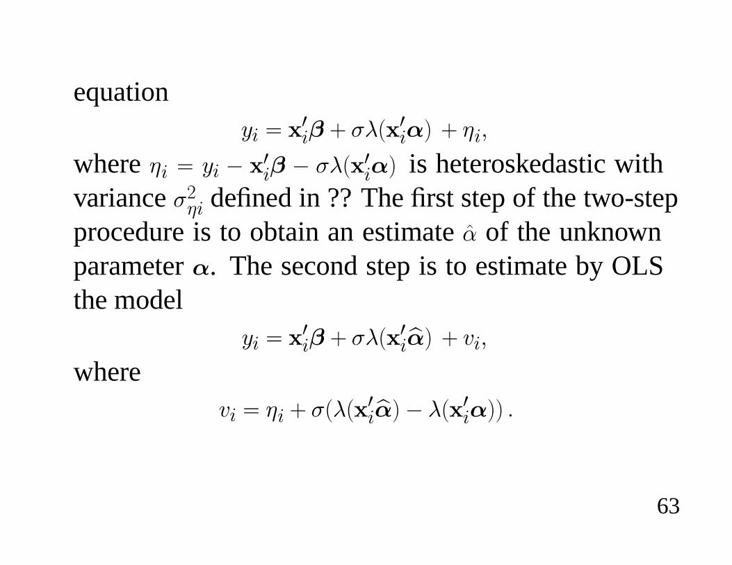
equation+� ' 3�� n jbE 3��� n #�c

where #� ' +� � 3�� � jbE 3��� is heteroskedastic withvariance j2#� de¿ned in ?? The ¿rst step of the two-stepprocedure is to obtain an estimatek of the unknownparameter�. The second step is to estimate by OLSthe model

+� ' 3�� n jbE 3�e�� n ��c

where�� ' #� n jEbE 3�e��� bE 3���� �

63

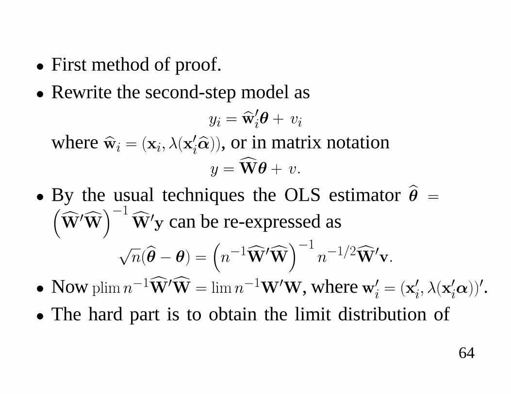
� First method of proof.

� Rewrite the second-step model as+� ' e�3

�� n ��

wheree�� ' E �c bE 3�e���, or in matrix notation

+ ' f̀� n ��

� By the usual techniques the OLS estimatore� '�f̀ 3f̀��� f̀ 3) can be re-expressed ass?Ee� � �� '

�?��f̀ 3f̀���

?��*2f̀ 3��

� NowT*�4?��f̀ 3f̀ ' *�4?��`3`, where�3� ' E 3�c bE 3����3.

� The hard part is to obtain the limit distribution of

64

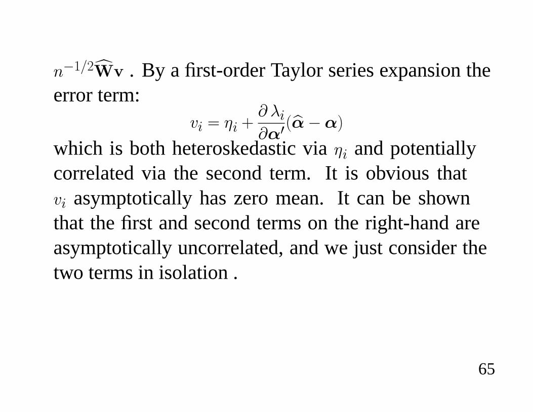
?��*2f̀� . By a ¿rst-order Taylor series expansion theerror term:

�� ' #� nY b�Y�3Ee����

which is both heteroskedastic via#� and potentiallycorrelated via the second term. It is obvious that�� asymptotically has zero mean. It can be shownthat the¿rst and second terms on the right-hand areasymptotically uncorrelated, and we just consider thetwo terms in isolation .

65

� It follows that?��*2f̀�

_$ 1kfc *�4?��`(d##3o` n *�4?��`#V�#`

lwhere # has �|� row #� ' Yb�*Y� and e� is asymptoti-cally 1d�cV�o.

� Combining these results gives the Heckman two-stepestimator e� @� 1 E�cV��c

whereV� is consistently estimated byeV� ' Ef̀ 3f̀���Ef̀ 3Pe#f̀ n f̀ 3 e#V� e#f̀�Ef̀ 3f̀���c

66

where f̀ 3f̀ '?S�'�

e��e�3�, f̀ 3 e# '

?S�'�

e��e_�, e_� ' Yb�E

3���*Y� me�

and Pe# is a diagonal matrix with �|� entry ej2# .� This estimate is straightforward to obtain if matrix

commands are available. The hardest part can beanalytically obtaining j2#� ' 9d#�o .

� If this is dif¿cult we can instead use ej2� ' �+� � 3�e� n ejb�E 3�e��

following the approach of White (1980).

67

� Second method of proof is to write the normal equa-tions for the two parts of the two-step estimator as

?[�'�

}E �c�� ' f

?[�'�

% �

b�

&E +� � 3�� n b�E

3���j� ' fc

where the¿rst equation is the¿rst-order conditionsfor � and the second equation gives OLS¿rst-orderconditions for�.

68

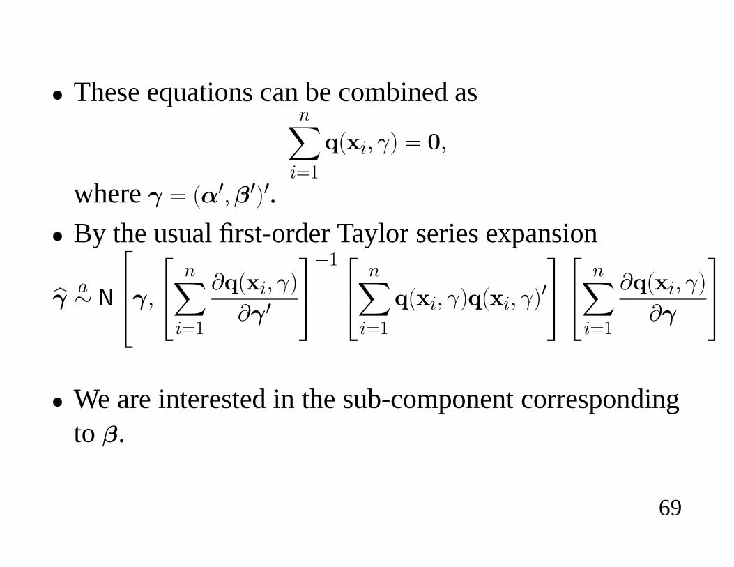
� These equations can be combined as?[�'�

^E �c �� ' fc

where � ' E�3c�3�3.� By the usual ¿rst-order Taylor series expansion

e� @� 1

597�c57 ?[�'�

Y^E �c ��

Y�3

68��57 ?[�'�

^E �c ��^E �c ��36857 ?[

�'�

Y^E �c ��

Y�

68� We are interested in the sub-component corresponding

to �.

69

� Simpli¿cation occurs because Y^E �c ��*Y� is blocktriangular because � does not appear in the ¿rst set ofequations. Newey (1984) gives the simpler formulaefor this case.

� Applying it to the example here will give the resultgiven earlier. Related papers are Pagan (1986) andMurphy and Topel (1985).

70