15682845 advanced excel 2000 user guide

Sponsor Message

www.remoteantispam.com TRY OUR HOSTED EMAIL SPAM BLOCKER

FREE FOR 14 DAYS

FOR BUSINESSES AND INDIVIDUALS WHO OWN THEIR INTERNET DOMAIN NAME

THE PROBLEM

Everybody hates spam email. Everybody. Even the people who send spam hate receiving it. Spam affects everybody, cluttering up inboxes and wasting time.

WHAT YOU CAN DO ABOUT IT

Doing something about spam is another matter. Most people rely on their service provider to protect their inboxes from spam, phishing, spyware and viruses.

But did you know that if you own your own email domain name Remote Anti Spam can block spam, viruses, spyware and phishing messages even before they get anywhere near your email system. Whether you’re an individual or a business.

Also, it doesn’t matter whether you have your own email server in your office or whether you use your ISP’s POP3 or IMAP4 service.

HOW DOES IT WORK?

Remote Anti Spam works by redirecting your emails to our global servers where they are filtered for spam, phishing, viruses and spyware. Messages containing these forms of unwanted content are rejected and discarded while your legitimate messages are forwarded on to your server for delivery to your mailbox.

There is no software to install on your server or on your computer or laptop. Nothing. You also don’t have to worry about downloading anything, setting anything up, configuring or updating. Ever. Just carry on doing what you were doing, but without the hassle of spam and harmful stuff getting in the way.

IT SOUNDS EXPENSIVE

It’s not. Quite the opposite. Visit our web site at www.remoteantispam.com for more information and pricing. What’s more is that we offer a 14 day free trial so you can check out the service to work out if it’s the correct solution for you.

Advanced Excel 2000 User Manual

Ebit Solutions Limited

December 1999

Ebit Solutions Limited www.ebitsolutions.net

IT Support London

Free Microsoft Office Training Manuals

EBIT SOLUTIONS LIMITED DECEMBER 1999

ADVANCED EXCEL 2000 USER MANUAL i

TABLE OF CONTENTS

INTRODUCTION 1 HOUSEKEEPING 1

NAMING RANGES 2 DEFINING A RANGE NAME 2 CREATING MULTIPLE RANGE NAMES 3

To ‘Create’ Range Names 3 MOVING TO AND SELECTING A NAMED RANGE 3 USING RANGE NAMES IN FORMULA 4

Intersecting Range Names Formula 4 APPLYING RANGE NAMES TO ALL YOUR FORMULAS 4

To Replace Cell References 4 DELETING RANGE NAMES 5 REDEFINING EXISTING RANGE NAMES 5

NAMING A FORMULA 6 To Name A Formula 6 To Use A Formula Name 6

GO TO 7 To Use Go To 7

SPECIAL GO TO FEATURES 8 To Use The Special Go To Options 8

FIND AND REPLACE 9 To Use Find And Replace 9

HIDING COLUMNS AND ROWS 10 To Hide A Column 10 To Hide A Row 10 To View (Unhide) A Column 10 To View (Unhide) A Row 10

GOAL SEEK 11 To Use Goal Seek 11

MOVING & COPYING SHEETS TO OTHER WORKBOOKS 12 To View Two Workbooks At The Same Time 12 To Move A Sheet 13 To Copy A Sheet 13 To Move Or Copy Multiple Sheets 13 To View Only One Workbook Again 13

LINKING WORKBOOKS 14 To Link Two Workbooks Together Using A Formula 14 To Link Several Workbooks Together 15

LINKING TO A WORD DOCUMENT 16 To Copy And Paste Link Data 16

DECEMBER 1999 EBIT SOLUTIONS LIMITED

ADVANCED EXCEL 2000 USER MANUAL ii

FORMULAS 17 ADVANCED FUNCTIONS 17

Rank 17 Trim 17 Concatenate 18 Sum If 18 And 18

LOOKUP TABLES 19

FUNCTIONS FOR CHANGING TEXT CASE 20 Upper 20 Lower 20 Proper 20

TURNING A FORMULA INTO ITS CALCULATED VALUE 21 To Turn A Formula Into A Value 21

NESTED FUNCTIONS 22 NESTED IF FUNCTION 22

THE FUNCTION WIZARD 23 To Use The Function Wizard 23 To Create A Formula Using The Function Wizard 25

MIXED CELL REFERENCES 26 EXAMPLE 26

To Create A Mixed Reference 26

VIEWING TOOLBARS 27 To View And Hide Toolbars 27

CUSTOMISING TOOLBARS 28 To Create A New Toolbar 28 To Add Buttons To A Toolbar 28 To Remove Buttons From A Toolbar 28

MACROS 29 To Record A Macro 29 To Run The Macro 30

EXAMPLE MACRO 31

ASSIGNING A MACRO TO A MACRO BUTTON 33 To Create A Macro Text Box 33

ASSIGNING A MACRO TO A TOOLBAR BUTTON 34 To Assign A Macro To A Toolbar Button 34


ADVANCED EXCEL 2000 USER MANUAL iii

SCENARIOS 35 To Create A Scenario 35 To View Scenarios 36 To Edit Scenarios 37 To Delete A Scenario 37

VIEWS 38 To Create A View 38 To Display The View 38

PRINT REPORTS 39 To Create A Print Report 39 To Print A Report 40

PIVOT TABLES AND PIVOT CHARTS 41 PIVOT TABLE EXAMPLE 41 PIVOT CHART EXAMPLE 42 CREATING A PIVOT TABLE OR CHART 42

To Create A Pivot Table or Chart 42 To Change The Way The Data Is Displayed In The Pivot Table 45 To Update The Pivot Table 45 To Delete A Pivot Table 45

USER-DEFINED CHART FORMATS 47 To Create Your Own Chart Format 47 To Apply User-Defined Chart Formats 48

PROTECTING SHEETS AND WORKBOOKS 49 To Protect A Whole Sheet 49 To Unprotect A Sheet 50

LOCKING AND UNLOCKING CELLS 50 To Lock Or Unlock Cells 50

TEXT TO COLUMNS 52 To Use Text To Columns 52

INSERTING HYPERLINKS 54 INSERTING AN E-MAIL CONTACT 55


ADVANCED EXCEL 2000 USER MANUAL 1

INTRODUCTION

The purpose of this manual is to introduce the more advanced techniques available in Excel 2000 for users who would like to increase their knowledge of this popular spreadsheet programme.

The advanced manual follows directly on from the Intermediate manual. Many of the topics covered here are introduced in the intermediate manual. A copy of the Intermediate manual can be requested from the IT Training department.

If you require more detailed instructions, or the complete range of topics, a full set of the Microsoft Office standard User Manuals is available in each office.

HOUSEKEEPING

Files created in Excel should be stored in your personal or shared areas on the network. This reduces the need to save or backup files onto floppy discs. You can obtain the names of your network drives from your colleagues, or you can request extra drives, in writing, from IT.

It is important that you save to the network drives as backups of information will take place daily. This reduces the likelihood of file loss via machine failure or theft.

Remember to delete old and unwanted files to free up space on the network.

www.ebitsolutions.net DECEMBER 1999 EBIT SOLUTIONS LIMITED

ADVANCED EXCEL 2000 USER MANUAL Block Spam reaching your inbox with Remote Anti Spam - www.remoteantispam.com/ftm

2

NAMING RANGES

Excel allows you to select a single cell, or a range of cells, and give it a name. You can then use the name to move to the cells and select them, or include them in a formula.

A formula containing lots of cell references can be confusing to look at and difficult to edit. But if the cell references are replaced by a range name it becomes much easier to understand.

For example the formula =SUM(B3:B24)-SUM(F3:F13) could be expressed as =TotalIncome-TotalExpenditure

DEFINING A RANGE NAME

You can name a single cell or a group of cells.

Select the cell(s) to name

In the “Insert” menu choose “Name”, then “Define”

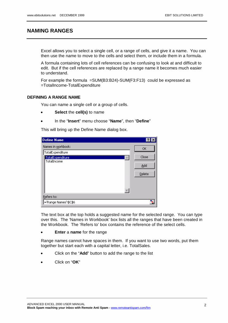
This will bring up the Define Name dialog box.

The text box at the top holds a suggested name for the selected range. You can type over this. The ‘Names in Workbook’ box lists all the ranges that have been created in the Workbook. The ‘Refers to’ box contains the reference of the select cells.

Enter a name for the range

Range names cannot have spaces in them. If you want to use two words, put them together but start each with a capital letter, i.e. TotalSales.

Click on the “Add” button to add the range to the list

Click on “OK”



CREATING MULTIPLE RANGE NAMES

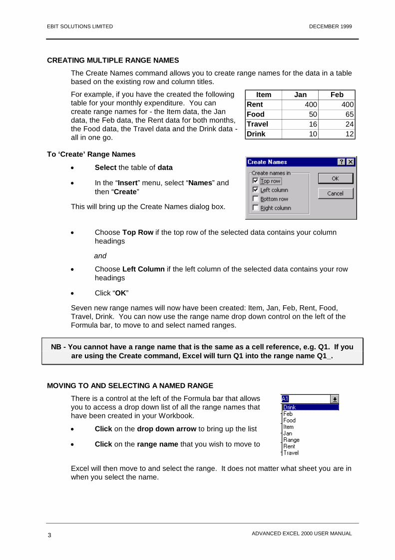
The Create Names command allows you to create range names for the data in a table based on the existing row and column titles.

For example, if you have the created the following table for your monthly expenditure. You can create range names for - the Item data, the Jan data, the Feb data, the Rent data for both months, the Food data, the Travel data and the Drink data - all in one go.

To ‘Create’ Range Names

Select the table of data

In the “Insert” menu, select “Names” and then “Create”

This will bring up the Create Names dialog box.

Item Jan FebRent 400 400Food 50 65Travel 16 24Drink 10 12

Choose Top Row if the top row of the selected data contains your column headings

and

Choose Left Column if the left column of the selected data contains your row headings

Click “OK”

Seven new range names will now have been created: Item, Jan, Feb, Rent, Food, Travel, Drink. You can now use the range name drop down control on the left of the Formula bar, to move to and select named ranges.

NB - You cannot have a range name that is the same as a cell reference, e.g. Q1. If you are using the Create command, Excel will turn Q1 into the range name Q1_.

MOVING TO AND SELECTING A NAMED RANGE

There is a control at the left of the Formula bar that allows you to access a drop down list of all the range names that have been created in your Workbook.

Click on the drop down arrow to bring up the list

Click on the range name that you wish to move to

Excel will then move to and select the range. It does not matter what sheet you are in when you select the name.



4

USING RANGE NAMES IN FORMULA

Having created a range name you can now use that name in a formula instead of cell references.

For example - if you have created the range name called “TotalIncome” for the cell containing the total income result, and a range name “TotalExpenditure” for cell containing the total expenditure, you can create a formula: =TotalIncome-TotalExpenditure (just by typing this text into a cell).

Another example - if you have created the range name “Costs” for all the cells in a column containing your costs data, you can calculate the total costs using the formula =Sum(Costs).

Intersecting Range Names Formula

Having created multiple range names (using the example on the previous page) the formula =Travel Jan would equal 16, the Travel figure for Jan (the value of the cell where the two named ranges intersect).

APPLYING RANGE NAMES TO ALL YOUR FORMULAS

If you have created range names after you have created some formulas in the workbook, you can replace all cell references with the new names in one go.

To Replace Cell References

Select all the cells containing formulas that you wish to change

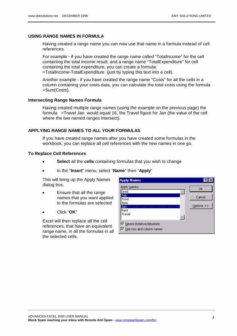
In the “Insert” menu, select “Name” then “Apply”

This will bring up the Apply Names dialog box.

Ensure that all the range names that you want applied to the formulas are selected

Click “OK”

Excel will then replace all the cell references, that have an equivalent range name, in all the formulas in all the selected cells.



DELETING RANGE NAMES

Range names are deleting using the Define Name dialog box.

In the “Insert” menu, select “Name” then “Define”

this will bring up the Define Name dialog box.

Select the name you wish to delete

Click on the “Delete” button

Repeat process for each name

Click “OK”

REDEFINING EXISTING RANGE NAMES

If you have added more data to a spreadsheet, and a range name no longer expresses the correct range of cells, you can redefine the named range.

In the “Insert” menu, select “Name”, then “Define” to bring up the Define Name dialog box

Select the range name you wish to redefine

In the Refers To box, change the reference to show the new range

TIP You can delete the existing reference and then click and drag through the new range on the spreadsheet, to enter it into the Refers To box.

Click “OK”



6

NAMING A FORMULA

Not only can you create names that refer to cell ranges, but you can also create a name that refers to a formula. This technique is useful when working with a complex formula (or perhaps one that acts on/tests a particular cell or range of cells). You can give the formula a short name and then recreate it any cell in the workbook by typing in that name.

To Name A Formula

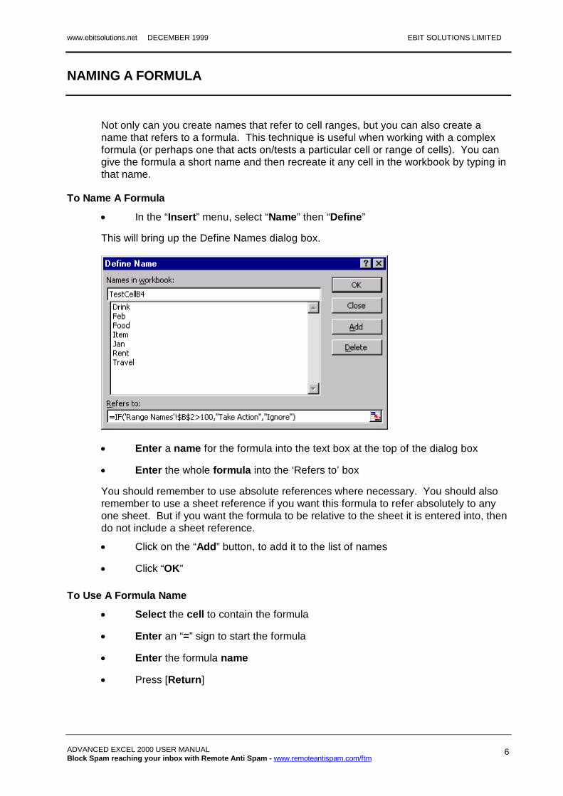
In the “Insert” menu, select “Name” then “Define”

This will bring up the Define Names dialog box.

Enter a name for the formula into the text box at the top of the dialog box

Enter the whole formula into the ‘Refers to’ box

You should remember to use absolute references where necessary. You should also remember to use a sheet reference if you want this formula to refer absolutely to any one sheet. But if you want the formula to be relative to the sheet it is entered into, then do not include a sheet reference.

Click on the “Add” button, to add it to the list of names

Click “OK”

To Use A Formula Name

Select the cell to contain the formula

Enter an “=” sign to start the formula

Enter the formula name

Press [Return]



GO TO

The Go To feature enables you to move to and select any cell or range of cells in your workbook. This feature is useful in large spreadsheets, as it can cut down on the time you spend scrolling around to find data.

To Use Go To

In the “Edit” menu select “Go To”

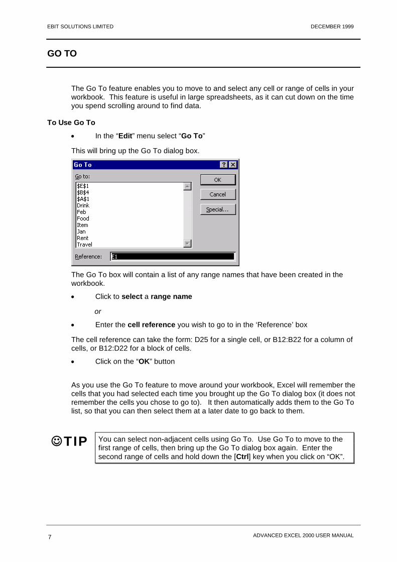
This will bring up the Go To dialog box.

The Go To box will contain a list of any range names that have been created in the workbook.

Click to select a range name

or

Enter the cell reference you wish to go to in the ‘Reference’ box

The cell reference can take the form: D25 for a single cell, or B12:B22 for a column of cells, or B12:D22 for a block of cells.

Click on the “OK” button

As you use the Go To feature to move around your workbook, Excel will remember the cells that you had selected each time you brought up the Go To dialog box (it does not remember the cells you chose to go to). It then automatically adds them to the Go To list, so that you can then select them at a later date to go back to them.

TIP You can select non-adjacent cells using Go To. Use Go To to move to the first range of cells, then bring up the Go To dialog box again. Enter the second range of cells and hold down the [Ctrl] key when you click on “OK”.



8

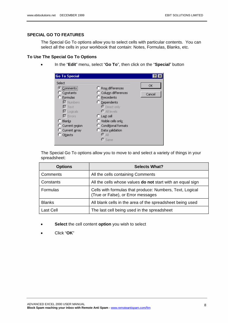
SPECIAL GO TO FEATURES

The Special Go To options allow you to select cells with particular contents. You can select all the cells in your workbook that contain: Notes, Formulas, Blanks, etc.

To Use The Special Go To Options

In the “Edit” menu, select “Go To”, then click on the “Special” button

The Special Go To options allow you to move to and select a variety of things in your spreadsheet:

Options Selects What?

Comments All the cells containing Comments

Constants All the cells whose values do not start with an equal sign

Formulas Cells with formulas that produce: Numbers, Text, Logical (True or False), or Error messages

Blanks All blank cells in the area of the spreadsheet being used

Last Cell The last cell being used in the spreadsheet

Select the cell content option you wish to select

Click “OK”



FIND AND REPLACE

Excel has a find and replace feature like Word. You can use it to search for a word, number or formula and then replace it with something else.

Find and Replace only works on the currently selected sheet(s).

To Use Find And Replace

Select the Sheet(s) you wish to search

In the “Edit” menu, select “Replace”

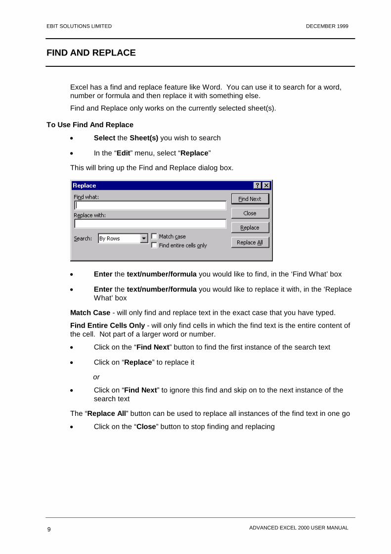
This will bring up the Find and Replace dialog box.

Enter the text/number/formula you would like to find, in the ‘Find What’ box

Enter the text/number/formula you would like to replace it with, in the ‘Replace What’ box

Match Case - will only find and replace text in the exact case that you have typed.

Find Entire Cells Only - will only find cells in which the find text is the entire content of the cell. Not part of a larger word or number.

Click on the “Find Next” button to find the first instance of the search text

Click on “Replace” to replace it

or

Click on “Find Next” to ignore this find and skip on to the next instance of the search text

The “Replace All” button can be used to replace all instances of the find text in one go

Click on the “Close” button to stop finding and replacing



10

HIDING COLUMNS AND ROWS

It is possible to hide a column or row of data to stop it printing out, or to stop other people from viewing it.

To Hide A Column

Select the column by clicking on the column heading

In the “Format” menu, select “Columns”, then “Hide”

The column will be hidden from view. But if you look at the column headings you can see which column is missing.

To Hide A Row

Select the column by clicking on the column heading

In the “Format” menu, select “Row”, then “Hide”

The row will be hidden from view. But if you look at the row headings you can see which row is missing.

You can hide multiple columns or rows at the same time - just select all the columns or rows at the same time and follow the steps outlined above.

To View (Unhide) A Column

The difficulty of bringing back a hidden column is that you need to select it first. As it is hidden, you cannot see the heading to click on it. The trick is to drag across the column headings either side of the hidden column. This will select the columns before and after the hidden column and the hidden column itself.

Click and drag across the column headings to select the columns before, the hidden column and the column after

In the “Format” menu, select “Column”, then “Unhide”

To View (Unhide) A Row

Similarly, the difficulty of bringing back a hidden row is that you need to select it first. As it is hidden, you cannot see the heading to click on it. The trick is to drag across the row headings either side of the hidden row. This will select the rows before and after the hidden row and the hidden row itself.

Click and drag across the row headings to select the rows before, the hidden row and the row after

In the “Format” menu, select “Row”, then “Unhide”



GOAL SEEK

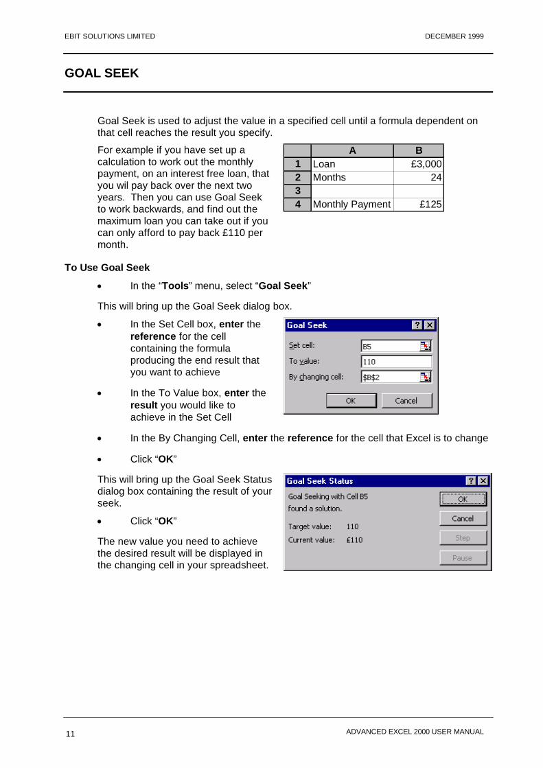
Goal Seek is used to adjust the value in a specified cell until a formula dependent on that cell reaches the result you specify.

For example if you have set up a calculation to work out the monthly payment, on an interest free loan, that you wil pay back over the next two years. Then you can use Goal Seek to work backwards, and find out the maximum loan you can take out if you can only afford to pay back £110 per month.

A B1 Loan £3,0002 Months 2434 Monthly Payment £125

To Use Goal Seek

In the “Tools” menu, select “Goal Seek”

This will bring up the Goal Seek dialog box.

In the Set Cell box, enter the reference for the cell containing the formula producing the end result that you want to achieve

In the To Value box, enter the result you would like to achieve in the Set Cell

In the By Changing Cell, enter the reference for the cell that Excel is to change

Click “OK”

This will bring up the Goal Seek Status dialog box containing the result of your seek.

Click “OK”

The new value you need to achieve the desired result will be displayed in the changing cell in your spreadsheet.



12

MOVING & COPYING SHEETS TO OTHER WORKBOOKS

The easiest way to move or copy sheets to other workbooks is to use drag and drop.

Drag and drop is commonly used to move cells around a spreadsheet, but it can also be used to move or copy sheets within the same workbook, or between different workbooks.

To drag and drop sheets between different workbooks, you need to have both workbooks open and visible on screen, at the same time.

To View Two Workbooks At The Same Time

Open the two workbooks that you wish to move or copy sheets between, but ensure that all other workbooks are closed

In the “Window” menu select “Arrange”

This will bring up the Arrange Windows dialog box.

Choose “Vertical” and click “OK”

This will display all workbooks currently open. Each workbook is displayed in its own window.



To Move A Sheet

Click and drag the sheet tab into the sheet tabs in the other workbook

A black triangle will appear marking the position at which the sheet will be positioned (between two sheets).

Release the mouse when the black triangle is at the correct position

If there is already a sheet with the same name in the workbook, Excel will call the incoming sheet version two, i.e. Sheet1 (2). You may wish to rename your sheets before you start moving them into other workbooks. (Double click on a sheet tab to rename it).

To Copy A Sheet

Follow the previous steps to make both workbooks visible on screen at once

Hold down the [Ctrl] key and then drag the sheet tab into the other workbook

Release the mouse (before you let go of the [Ctrl] key)

A copy of the sheet will have been inserted into the other workbook.

To Move Or Copy Multiple Sheets

You can select multiple sheets and move or copy them all at the same time.

Select the first sheet you wish to move/copy

Hold down the [Ctrl] key and click on each additional sheet tab you wish to select

When all the necessary sheets are selected.

Release the [Ctrl] key

Click and drag on one of the selected sheet tabs to start the move.

If you wish to copy the sheets, hold down the [Ctrl] key while you are in the middle of the dragging process

If you hold down the [Ctrl] key before you start dragging, Excel thinks you are trying to deselect the sheet you are clicking on.

Release the mouse over the sheet tabs in the other workbook

To View Only One Workbook Again

Click on the maximise button for the workbook you wish to view

It will fill the Excel window. The other workbook will remain open, layered behind the visible workbook, and can be accessed via the “Window” menu.



14

LINKING WORKBOOKS

If you need to, you can link two workbooks together. This can be done by creating a formula that contains the reference for a cell that is in another workbook.

This method allows you to pull in important calculations/values from other workbooks. Because a reference is used the value will update if the content of the cell being referred to changes.

If you have linked two files together, you should not start moving either of the files around (into other drives or directories). If you do, Excel will not be able to find the file

that has been moved, and will be unable to maintain the link.

Before you start linking workbooks together you need to think about what will happen to the workbooks in the long term. Will other people be using them? Will they be making copies? Will they be mailing copies to other people? If the answers to these questions

are “yes”, then perhaps you should avoid creating a link.

You have been warned!!!

To Link Two Workbooks Together Using A Formula

You have a workbook that contains a value that you wish to link to and display in another workbook.

Open both workbooks

In the workbook you wish to display the value in

Click to select the cell you would like to display the value in

Start the formula by typing =

In the “Windows” menu, select the workbook containing the value you want to link to

Click on the cell containing the value

The reference for this cell will be inserted into the formula in the form: =[ACCOUNTS.XLS]Sheet1!$B$6

The workbook name is expressed in square brackets. The sheet name is expressed with an exclamation mark after it, followed by the cell reference expressed as an absolute reference (with dollar sign before the column and row reference).

Press [Return] to finish the formula

Whatever appears in the cell B6 in Sheet1 in the Accounts workbook will be shown in the cell containing this formula.

To remove the link, delete the formula.



To Link Several Workbooks Together

You could add up cells in different workbooks and put the result in a new workbook.

Click on the cell to contain the final result

Type in = and move to each workbook that contains a cell you want to include in the formula. Click on each cell you wish to include, typing in +, -, * or / (depending on what you want to do) between each cell reference

Press [Return] to finish the formula

The final formula could take the form: =[ACCS95.XLS]Sheet1!$E$55+[ACCS96.XLS]Sheet1!$G$84



16

LINKING TO A WORD DOCUMENT

You should already know how to copy and paste Excel spreadsheet cells into a Word document. They will appear in the document as a word table, and can then be edited or formatted using the Word table commands.

It is also possible to copy and paste link Excel data into a Word document. The data in your document will maintain a link with the Excel workbook that it came from, and will update automatically if the data changes in the workbook.

To Copy And Paste Link Data

In Excel, select the cells to link

Click on the “Copy” button

Move to Word using the word button on the start bar

Click in the document to position the text insertion point

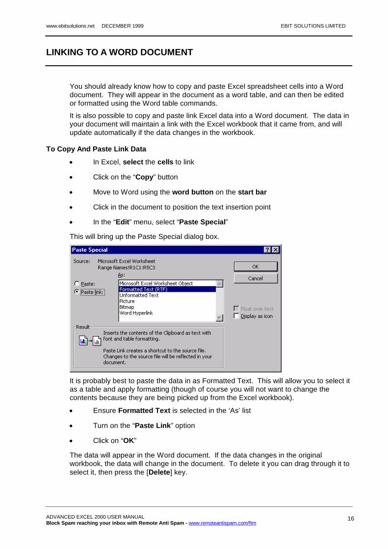
In the “Edit” menu, select “Paste Special”

This will bring up the Paste Special dialog box.

It is probably best to paste the data in as Formatted Text. This will allow you to select it as a table and apply formatting (though of course you will not want to change the contents because they are being picked up from the Excel workbook).

Ensure Formatted Text is selected in the ‘As’ list

Turn on the “Paste Link” option

Click on “OK”

The data will appear in the Word document. If the data changes in the original workbook, the data will change in the document. To delete it you can drag through it to select it, then press the [Delete] key.



Do not change the location of files containing data that is linked together

FORMULAS

ADVANCED FUNCTIONS

Excel contains over three hundred different formula codes, called functions. You will be familiar with the most common function, SUM, used to total a range of cells. Here are some others that I have found to be useful.

Rank

The Rank function is used to discover the rank or position of a number in a range of numbers.

The formula takes the form: =RANK(number,range,order)

Where number is the reference of the cell whose rank you wish to find, range is the range of numbers, and order is used to rank the order by greatest or smallest number. The order component is not compulsory. If order is 0 or left blank then the largest number in the range is ranked first. If order is 1 then the smallest number in the range is ranked first.

For example, if you have a list of ten numbers in the range A1:A10, and the number in the cell A1 is the largest number in the range, then:

=RANK(A1,A1:A10) will equal 1

=RANK(A1,A1:A10,0) will equal 1

=RANK(A1,A1:A10,1) will equal 10

Trim

The Trim function is used to remove all the spaces from text except for single spaces between words.

It seems to be quite a common problem that people type extra spaces, either before or after words, when inputting data. This can prevent Excel from being able to sort data properly, and can also disrupt subtotalling.

The formula takes the form: =TRIM(text)

Where text is the reference of a cell containing text.

For example, if cell A1 contains the text “ Total Annual Sales ”, then:

=TRIM(A1) equals “Total Annual Sales”



18

Concatenate

The Concatenate function is used to create a text string, in one cell, from the contents of different cells.

The formula takes the form: =CONCATENATE(text1,text2,...)

Where text1 can be a cell references, or text in inverted commas.

For example, if cell B2 contains the word Total, and cell C2 contains the word Value, and D2 contains the number 450, then:

=CONCATENATE(B2,C2) will equal “TotalValue”

=CONCATENATE(B2,“ ”,C2) will equal “Total Value”

=CONCATENATE(B2,“ ”,C2,“ is equal to ”,D2) will equal “Total Value is equal to 450”

Sum If

The Sum If function is used to add the cells that match a specified criteria.

The formula takes the form: =SUMIF(range,criteria,sum_range)

Where range is the range of cells you want to evaluate, criteria is the criteria by which you wish to evaluate the cells, and sum_range is the range of cells that you wish to add up. The criteria can be evaluating a number or text, and can be expressed as 25, “25”, “>25” or “Product A”. Only the cells in the sum_range that satisfy the criteria will be added up.

For example, if cells A1:A10 contain either the words “Product A” or “Product B”, and cells B1:B10 contain different prices, then:

=SUMIF(A1:A10,“Product A”,B1:B10) will equal the total price for all the Product A items.

And

The And formula is used to test other cells. If all the cells being tested satisfy the test, the formula will equal True. If at least one of the cells being tested does not satisfy the test, the formula will equal False.

The formula takes the form: =AND(test1,test2,test3, ...)

Where test is the test you want to perform. You can use the conditional operators to test the contents of cells: = < > <= >= <>.

For example, if cell A1 contains the number 50, and cell A2 contains 120, and cell B1 contains the word House, then:

=AND(A1>0,A2>100) will equal True

=AND(A1>100,A2>100) will equal False

=AND(B1=“House”,A1<100,A2>100) will equal True



LOOKUP TABLES

Lookup is a formula function that is used to lookup values in a table or array.

The formula takes the form:

=LOOKUP(lookup_value,lookup_vector,lookup_result)

Where:

lookup_value is the value you wish to look up. This can be a number or text.

lookup_vector is the range you wish to look up in. This can contain numbers or text.

lookup_result is the range to find the range to look up the result in. This can contain numbers or text.

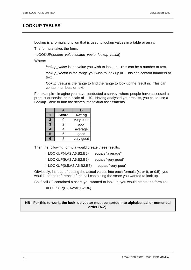
For example - Imagine you have conducted a survey, where people have assessed a product or service on a scale of 1-10. Having analysed your results, you could use a Lookup Table to turn the scores into textual assessments.

A B1 Score Rating2 0 very poor3 2 poor4 4 average5 6 good6 8 very good

Then the following formula would create these results:

=LOOKUP(4,A2:A6,B2:B6) equals “average”

=LOOKUP(9,A2:A6,B2:B6) equals “very good”

=LOOKUP(0.5,A2:A6,B2:B6) equals “very poor”

Obviously, instead of putting the actual values into each formula (4, or 9, or 0.5), you would use the reference of the cell containing the score you wanted to look up.

So if cell C2 contained a score you wanted to look up, you would create the formula:

=LOOKUP(C2,A2:A6,B2:B6)

NB - For this to work, the look_up vector must be sorted into alphabetical or numerical order (A-Z).



20

FUNCTIONS FOR CHANGING TEXT CASE

The next three formulas are used to change the case of text. This can be useful if large amounts of data have been inputted in the wrong case. Once the case has been changed using these formulas, you will need to turn the result of the formula into text again. (See bottom of page).

Alternatively, instead of using the formula, you could copy the data and paste it into Word, use the Change Case options in the Format menu to change the case and then copy and paste the data back into Excel.

Upper

The Upper function is used to make text uppercase.

The formula takes the form: =UPPER(text)

Where text is the reference for a cell containing text.

For example, if cell A1 contains the text “value”, then:

=UPPER(A1) equals “VALUE”

Lower

The Lower function is used to make text lowercase.

The formula takes the form: =LOWER(text)


For example, if cell A1 contains the text “VALUE”, then:

=LOWER(A1) equals “value”

Proper

The Proper function is used to make text title case.

The formula takes the form: =PROPER(text)


For example, if cell A1 contains the text “total value”, then:

=PROPER(A1) equals “Total Value”

Once the case has been changed, you will need to turn the result of the formula into text again. (See next section).



TURNING A FORMULA INTO ITS CALCULATED VALUE

If you have created a formula that produces a text or numerical result, you can turn the result into the calculated value, so that it is no longer a formula.

You can either do this in a different cell (thereby leaving the original formula alone), or you can do it over the original cell.

To Turn A Formula Into A Value

Select the cell(s) containing the formula

Click on the “Copy” button

If you want to replace the formula with the value.

Keep the cell(s) selected

If you want to leave the original formula alone.

Click on an empty cell to select a new paste area

In the “Edit” menu select “Paste Special”

Select the “Values” option

Click “OK”



22

NESTED FUNCTIONS

Excel allows you to include more than one function in a formula. For example you can add two totals using the formula: =SUM(A1:A2)+SUM(B1:B2). But this does not make it a nested formula.

A ‘nested’ formula is one in which a function is included in the argument of another function. This technique allows you to build more complex formula.

Argument(s) appear in brackets after the function. Some functions require several arguments, some require only one. An argument can be a number, a reference, or text (usually in inverted commas). If a formula has more than one argument they will be separated by commas. Here are some examples:

=SUM(A3:A23) This formula has one argument - a reference

=SUMIF(A1:A10,“Product A”,B1:B10) This formula has three arguments - a reference, text, and another reference.

Here is an example of a nested function, containing another function in an argument. This calculates the average of two totals:

=AVERAGE(SUM(A3:A23),SUM(D3:D23))

A useful example of a nested function is a nested IF function.

NESTED IF FUNCTION

The IF function can normally be used to test a cell and perform two different actions depending on the outcome of the test. (See Intermediate Manual for introduction to the IF Function). But by nesting another IF function inside an IF function you can test a cell and perform three different actions depending on the outcome of the tests. You can actually nest up to 7 functions within a formula. So you could actually perform up to seven different actions, depending on the result of the test.

The basic IF formula takes the form: =IF(condition to test,action if true,action if false)

So the formula: =IF(A1>0,B1*2,B1*3) tests cell A1 to see if is greater than 0. If it is, cell B1 is multiplied by 2. If it is not, cell B1 is multiplied by 3.

To create a nested IF function we insert another IF formula into the “action if true” argument. The result could look like this:

=IF(A1>0,IF(A1>100,B1*4,B1*3),B1*2)

Given that cell B1 contains the number 2, then: if cell A1 contains the number 25, the result would be 6 if cell A1 contains the number 200, the result would be 8 if cell A1 contains the number -12, the result would be 4

Thus the formula tests cell A1 to see if it is greater or less than zero. If it is greater than zero, it is then tested again to see if it is greater than 100. Three actions can then occur depending on the value of cell A1.



THE FUNCTION WIZARD

The Function Wizard can be used to guide you through creating a formula. For basic formula it is generally easier to type the formula straight into the spreadsheet cell. But for complex formula it can be helpful to use the Wizard and build the formula step by step.

The Function Wizard can also be used to learn new formula, as it contains a list of all the existing Excel formulas and a description and example of each one.

To Use The Function Wizard

Select the cell to contain the formula

Click on the “Function Wizard” button

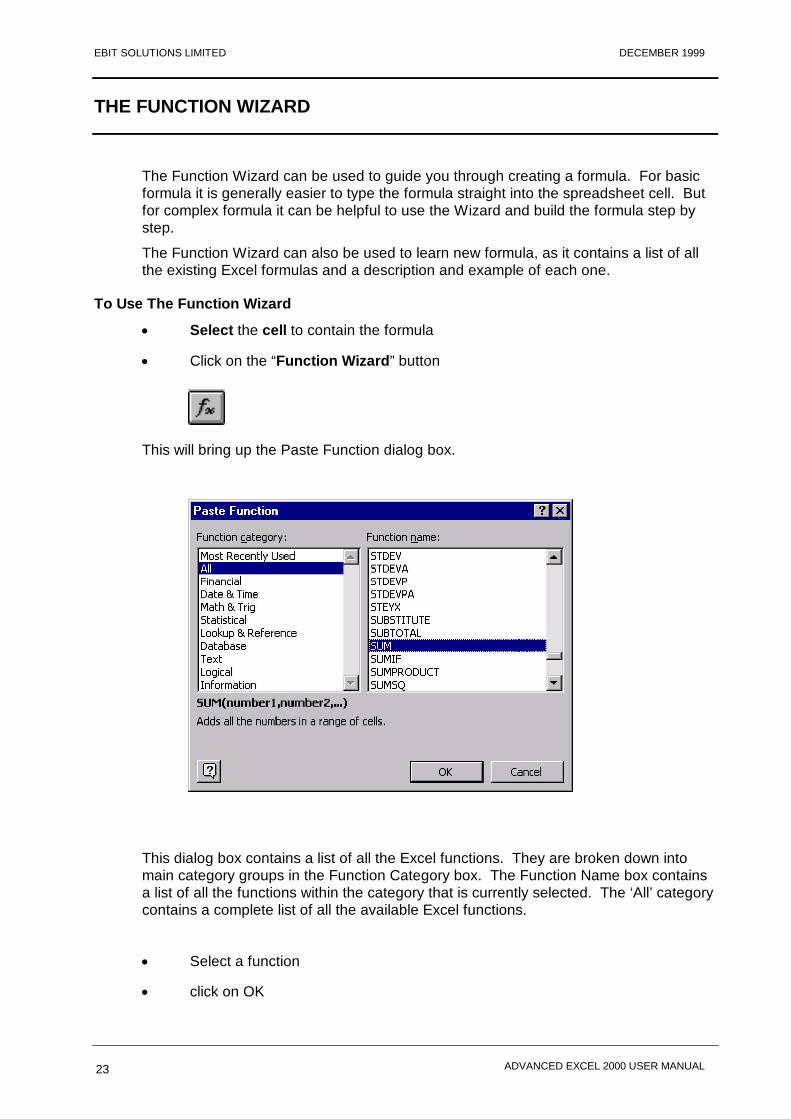
This will bring up the Paste Function dialog box.

This dialog box contains a list of all the Excel functions. They are broken down into main category groups in the Function Category box. The Function Name box contains a list of all the functions within the category that is currently selected. The ‘All’ category contains a complete list of all the available Excel functions.

Select a function

click on OK



24

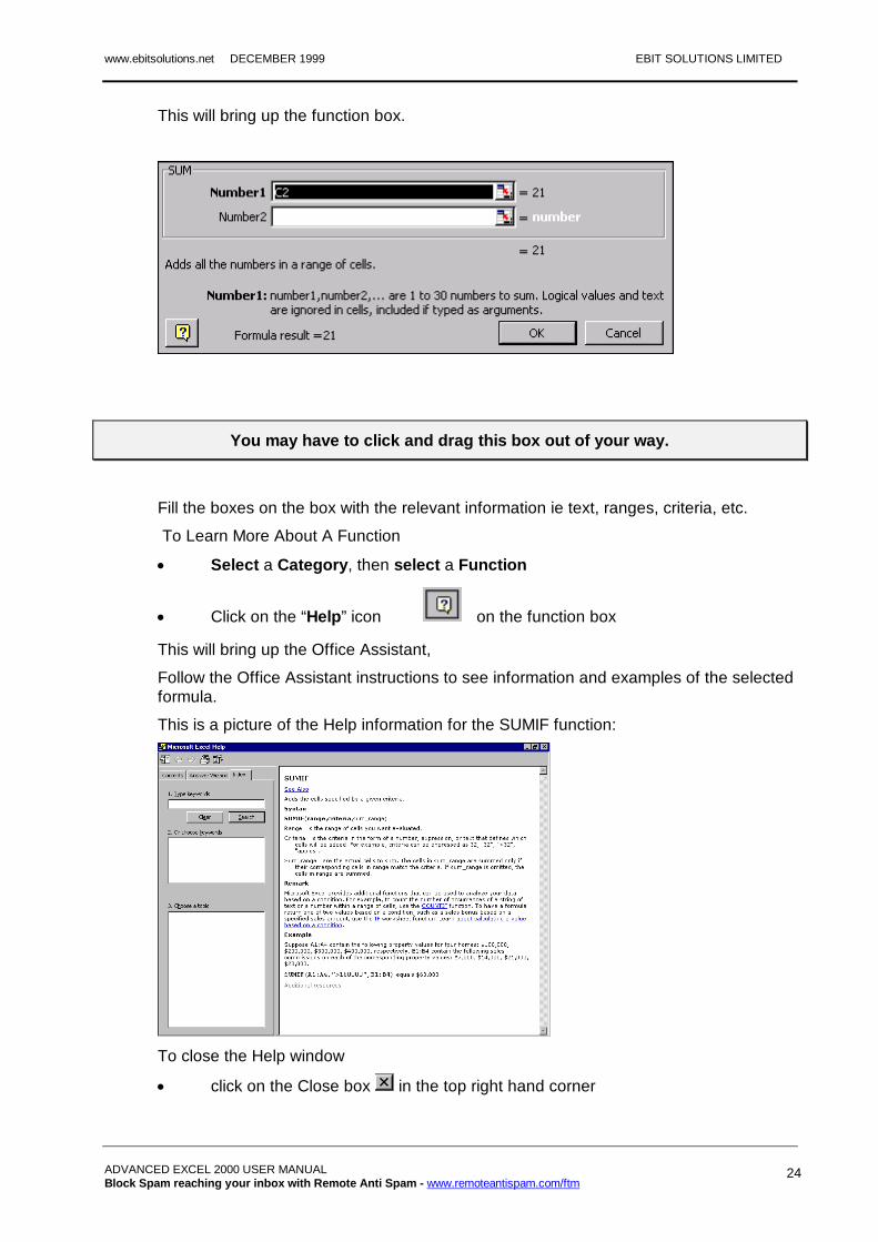
This will bring up the function box.

You may have to click and drag this box out of your way.

Fill the boxes on the box with the relevant information ie text, ranges, criteria, etc.

To Learn More About A Function

Select a Category, then select a Function

Click on the “Help” icon on the function box

This will bring up the Office Assistant,

Follow the Office Assistant instructions to see information and examples of the selected formula.

This is a picture of the Help information for the SUMIF function:

To close the Help window

click on the Close box in the top right hand corner



To Create A Formula Using The Function Wizard

In step 1 of the Function Wizard.

Select a Category

Select a Function

Click on the “OK” button

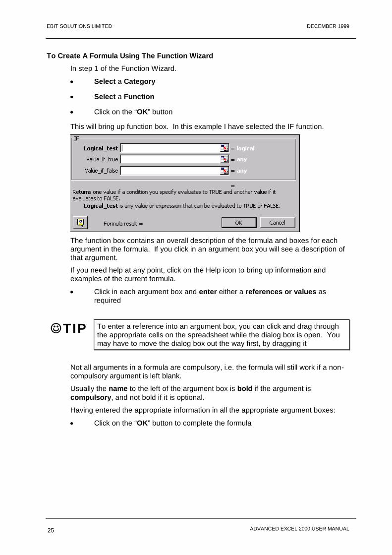
This will bring up function box. In this example I have selected the IF function.

The function box contains an overall description of the formula and boxes for each argument in the formula. If you click in an argument box you will see a description of that argument.

If you need help at any point, click on the Help icon to bring up information and examples of the current formula.

Click in each argument box and enter either a references or values as required

TIP To enter a reference into an argument box, you can click and drag through the appropriate cells on the spreadsheet while the dialog box is open. You may have to move the dialog box out the way first, by dragging it

Not all arguments in a formula are compulsory, i.e. the formula will still work if a non-compulsory argument is left blank.

Usually the name to the left of the argument box is bold if the argument is compulsory, and not bold if it is optional.

Having entered the appropriate information in all the appropriate argument boxes:

Click on the “OK” button to complete the formula



26

MIXED CELL REFERENCES

An absolute cell reference in a formula, fixes the reference on a particular column and a particular row. When the formula is copied to another cell it then continues to refer to exactly the same cell. An absolute reference takes the form $B$4.

A mixed cell reference fixes the reference on a column or on a row, but not both at the same time. A mixed reference takes the form $B4 (fixed on column B but not on any row) or B$4 (fixed on row 4 but not on any column).

EXAMPLE

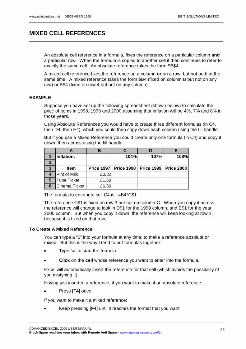
Suppose you have set up the following spreadsheet (shown below) to calculate the price of items in 1998, 1999 and 2000 assuming that inflation will be 4%, 7% and 8% in those years.

Using Absolute References you would have to create three different formulas (in C4, then D4, then E4), which you could then copy down each column using the fill handle.

But if you use a Mixed Reference you could create only one formula (in C4) and copy it down, then across using the fill handle.

A B C D E1 Inflation: 104% 107% 108%23 Item Price 1997 Price 1998 Price 1999 Price 20004 Pint of Milk £0.325 Tube Ticket £1.606 Cinema Ticket £6.50

The formula to enter into cell C4 is: =B4*C$1

The reference C$1 is fixed on row 3 but not on column C. When you copy it across, the reference will change to look in D$1 for the 1999 column, and E$1 for the year 2000 column. But when you copy it down, the reference will keep looking at row 1, because it is fixed on that row.

To Create A Mixed Reference

You can type a “$” into your formula at any time, to make a reference absolute or mixed. But this is the way I tend to put formulas together:

Type “=“ to start the formula

Click on the cell whose reference you want to enter into the formula.

Excel will automatically insert the reference for that cell (which avoids the possibility of you mistyping it).

Having just inserted a reference, if you want to make it an absolute reference:

Press [F4] once

If you want to make it a mixed reference:

Keep pressing [F4] until it reaches the format that you want



VIEWING TOOLBARS

Excel contains many toolbars. The Standard and Formatting Toolbars are visible all the time, and other toolbars usually appear when you initiate certain tasks. For instance when you create a chart, Excel should bring up the Chart Toolbar. When you create a pivot table, Excel should bring up the Query and Pivot Toolbar (see section on Pivot Tables).

In case a toolbar does not appear when it should, or in case you close one down accidentally, it is useful to know how to view and hide toolbars.

To View And Hide Toolbars

In the “View” menu, select “Toolbars”

This will bring up the futher menu, containing a list of all the existing toolbars. Toolbars with ticks in the box beside them are selected and are displayed on screen.

Click to select or deselect the toolbar you wish to view

Click “OK”

You can create your own personal toolbar, to which you can add all the buttons you find most useful. (See next section, on Customising Toolbars).



28

CUSTOMISING TOOLBARS

As well as containing many toolbars, Excel also contains many different toolbar buttons, some of which are not shown on any existing toolbars.

You may find that there are some toolbar buttons that would be useful for you. If so, you can add them to an existing toolbar, or create a new personal toolbar to put them on. You can also create your own buttons and assign macros to them. (See section on Assigning A Macro To A Toolbar Button)

To Create A New Toolbar

In the “View” menu, select “Toolbars”

In the Toolbars list, select Customise

Click on the New button

Give the toolbar an appropriate name in the dialog box that appears

The new toolbar will appear on screen. It will probably appear as a free-floating toolbar, with a blue title bar and a small control button. You can click and drag on the title bar to move the toolbar into a new position. You can click on the control button to close the toolbar.

To Add Buttons To A Toolbar

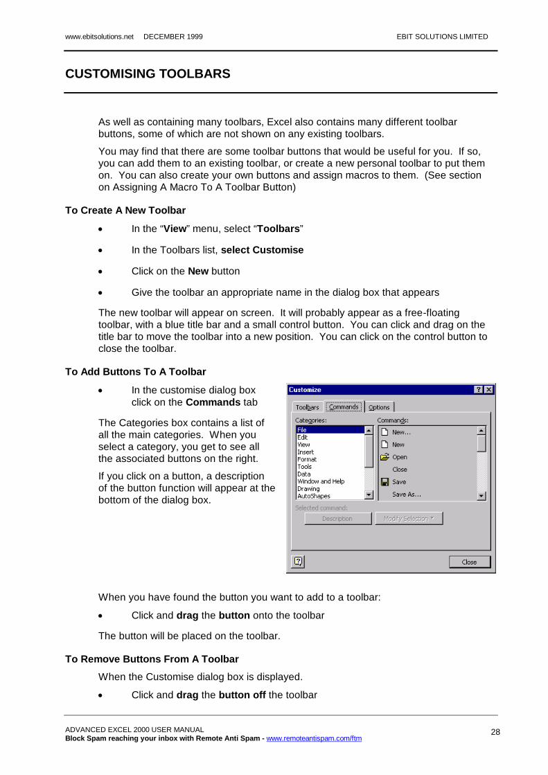
In the customise dialog box click on the Commands tab

The Categories box contains a list of all the main categories. When you select a category, you get to see all the associated buttons on the right.

If you click on a button, a description of the button function will appear at the bottom of the dialog box.

When you have found the button you want to add to a toolbar:

Click and drag the button onto the toolbar

The button will be placed on the toolbar.

To Remove Buttons From A Toolbar

When the Customise dialog box is displayed.

Click and drag the button off the toolbar



MACROS

A macro is a collection of commands that are performed in a set order.

If you find you are performing the same commands/actions over and over again, in exactly the same sequence, you can create a macro to record all those actions for you. You can then assign the macro to a toolbar button and then run the macro using a single click. You can also assign the macro to a keyboard command.

For example a simple macro could be to select a particular range of cells and print them out. There are five steps in this macro: select the range, choose “File” menu, choose “Print” command, choose “Print Selection”, click on “OK”.

There are two ways of creating a macro. You can record the actions in the sequence that you want them to be performed, or you can use the macro programming language Visual Basic to write a macro. We are just going to look at the first method.

You will need to understand Range Names if you are going to start creating macros. See section on ‘Naming Ranges’.

To Record A Macro

These are the generic steps to create a simple macro. After that I will guide you through the steps to create an example macro to select and print a particular range of cells.

Before you start, ensure that any range of cells that need to be selected in the macro have been given a range name. (See section on Naming Ranges).

In the “Tools” menu, choose “Macro”, then “Record New Macro”

This will bring up the Record Macro dialog box.

Excel will come up with the suggested name Macro1. You can type over this.

Macro names must be one word with no spaces. It is best to give the macro a name that relates to what it does, i.e. PrintAccountsData, rather than a non-descriptive name such as Macro1.

Type a name for the macro into the Macro Name box

You can add the macro to the Tools drop down menu, by turning on the ‘Assign Menu Item’ option and typing a command name for the macro in the box. The command will appear at the bottom of the Tools menu.



30

You can give the macro a keyboard shortcut command by turning on the Assign Shortcut Key command, and entering a letter into the ‘Ctrl+’ box. Do not use any letters that are already in use. Only half the alphabet is left: D, E, I, J, K, L, M, Q, R, T, W, Y.

If desired, enter a letter into the ‘Ctrl+‘ box

You can also assign a macro to a toolbar button, or create a Text box in the spreadsheet that can be clicked on to run the macro. This is done after the macro has been recorded. (See section on Assigning A Macro To A Toolbar Button).

Macros can be stored in the current workbook, which makes them only available in that workbook, or they can be stored in the Personal Macro Workbook, which will make them available in all workbooks on your computer. If you store a macro in the Personal Macro Workbook, this macro workbook will then open up each time you start up Excel.

Select “This Workbook” or “Personal Macro Workbook” as appropriate

Click on “OK”

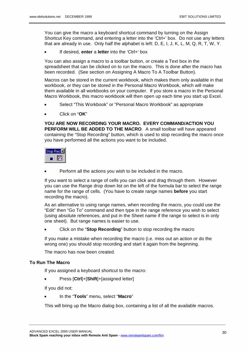
YOU ARE NOW RECORDING YOUR MACRO. EVERY COMMAND/ACTION YOU PERFORM WILL BE ADDED TO THE MACRO. A small toolbar will have appeared containing the “Stop Recording” button, which is used to stop recording the macro once you have performed all the actions you want to be included.

Perform all the actions you wish to be included in the macro.

If you want to select a range of cells you can click and drag through them. However you can use the Range drop down list on the left of the formula bar to select the range name for the range of cells. (You have to create range names before you start recording the macro).

As an alternative to using range names, when recording the macro, you could use the “Edit” then “Go To” command and then type in the range reference you wish to select (using absolute references, and put in the Sheet name if the range to select is in only one sheet). But range names is easier to use.

Click on the “Stop Recording” button to stop recording the macro

If you make a mistake when recording the macro (i.e. miss out an action or do the wrong one) you should stop recording and start it again from the beginning.

The macro has now been created.

To Run The Macro

If you assigned a keyboard shortcut to the macro:

Press [Ctrl]+[Shift]+[assigned letter]

If you did not:

In the “Tools” menu, select “Macro”

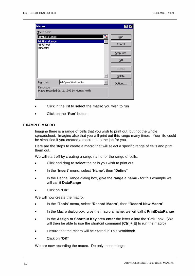
This will bring up the Macro dialog box, containing a list of all the available macros.



Click in the list to select the macro you wish to run

Click on the “Run” button

EXAMPLE MACRO

Imagine there is a range of cells that you wish to print out, but not the whole spreadsheet. Imagine also that you will print out this range many times. Your life could be simplified if you created a macro to do the job for you.

Here are the steps to create a macro that will select a specific range of cells and print them out.

We will start off by creating a range name for the range of cells.

Click and drag to select the cells you wish to print out

In the “Insert” menu, select “Name”, then “Define”

In the Define Range dialog box, give the range a name - for this example we will call it DataRange

Click on “OK”

We will now create the macro.

In the “Tools” menu, select “Record Macro”, then “Record New Macro”

In the Macro dialog box, give the macro a name, we will call it PrintDataRange

In the Assign to Shortcut Key area enter the letter e into the ‘Ctrl+’ box. (We will then be able to use the shortcut command [Ctrl]+[E] to run the macro)

Ensure that the macro will be Stored in This Workbook

Click on “OK”

We are now recording the macro. Do only these things:



32

Click on the drop down range name arrow on the left of the formula bar, and select the range DataRange (that we created earlier)

Select the “File” menu, then choose “Print”

In the Print Dialog box, select the “Print Selection” option

Click “OK” to print

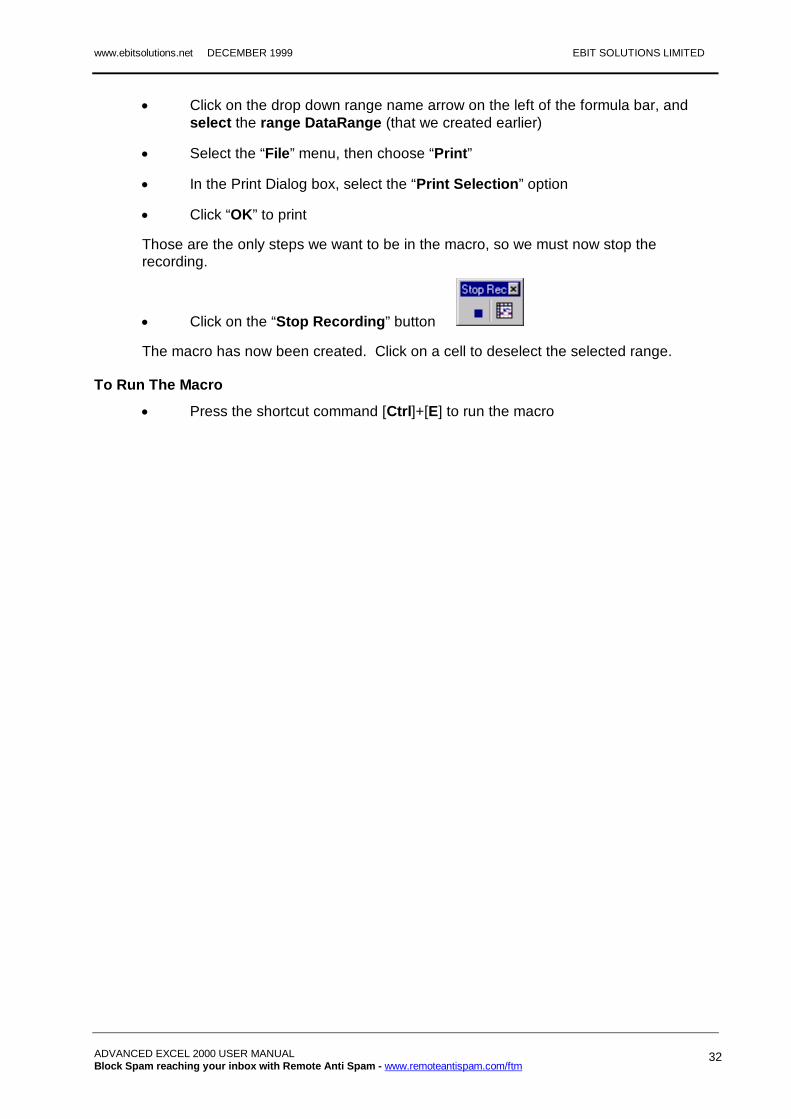
Those are the only steps we want to be in the macro, so we must now stop the recording.

Click on the “Stop Recording” button

The macro has now been created. Click on a cell to deselect the selected range.

To Run The Macro

Press the shortcut command [Ctrl]+[E] to run the macro



ASSIGNING A MACRO TO A MACRO BUTTON

Having created a macro in your workbook you can create a button, on the spreadsheet, that can be used to run the macro. This will stop you having to remember a keyboard shortcut or fill the Tools menu up with macro commands.

To Create A Macro Text Box

We need to use the Drawing Toolbar

Click on the Drawing Toolbar button in the Standard Toolbar

This will bring up the Drawing Toolbar.

Click on a Drawing shape

Click and drag over the spreadsheet to create the shape

When you let go of the mouse button, you should add the appropriate Text and format the shape with colour, shadow, etc.

Right click on the shape to assign a macro

Click on “Assign Macro”

The Assign Macro dialog box will appear



34

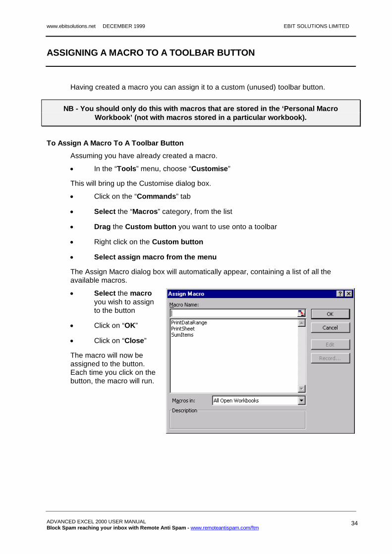
ASSIGNING A MACRO TO A TOOLBAR BUTTON

Having created a macro you can assign it to a custom (unused) toolbar button.

NB - You should only do this with macros that are stored in the ‘Personal Macro Workbook’ (not with macros stored in a particular workbook).

To Assign A Macro To A Toolbar Button

Assuming you have already created a macro.

In the “Tools” menu, choose “Customise”

This will bring up the Customise dialog box.

Click on the “Commands” tab

Select the “Macros” category, from the list

Drag the Custom button you want to use onto a toolbar

Right click on the Custom button

Select assign macro from the menu

The Assign Macro dialog box will automatically appear, containing a list of all the available macros.

Select the macro you wish to assign to the button

Click on “OK”

Click on “Close”

The macro will now be assigned to the button. Each time you click on the button, the macro will run.



SCENARIOS

If you have created a spreadsheet that contains data that is not yet known, but will affect subsequent calculations, you can create different scenarios to calculate best and worst case outcomes.

For example if you are creating a personal budget for next year, but do not know what your mortgage payments will be due to the changing rate of interest, or how much your rail card with cost. You can define different scenarios and then switch between them to do ‘what-if’ analysis to see if you will end up in debt or be able to afford a holiday.

Obviously this is a simple example. Scenarios work best on complex spreadsheets where there is a large knock-on effect from changes in the variable data.

Scenarios are created and managed using the Scenario Manager.

To Create A Scenario

Create and format the spreadsheet.

You can leave the variable cells empty. (These are cells B6 and B8 in the example above).

In the “Tools” menu, select “Scenarios”

This will bring up the Scenario Manager dialog box.

Click on the “Add” button, to create a new scenario

This will bring up the Add Scenario dialog box.



36

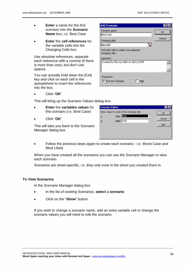
Enter a name for the first scenario into the Scenario Name box, i.e. Best Case

Enter the cell references for the variable cells into the Changing Cells box

Use absolute references, separate each reference with a comma (if there is more than one), but don’t use spaces.

You can actually hold down the [Ctrl] key and click on each cell in the spreadsheet to insert the references into the box.

Click “OK”

This will bring up the Scenario Values dialog box.

Enter the variables values for this scenario (i.e. Best Case)

Click “OK”

This will take you back to the Scenario Manager dialog box.

Follow the previous steps again to create each scenario - i.e. Worst Case and

Most Likely

When you have created all the scenarios you can use the Scenario Manager to view each scenario.

Scenarios are sheet-specific, i.e. they only exist in the sheet you created them in.

To View Scenarios

In the Scenario Manager dialog box.

In the list of existing Scenarios, select a scenario

Click on the “Show” button

If you wish to change a scenario name, add an extra variable cell or change the scenario values you will need to edit the scenario.



To Edit Scenarios

In the Scenario Manager dialog box.


Click on the “Edit” button

This will bring up the Edit Scenario dialog box, in which you can change the scenario name or alter the changing cells

Make the changes

Click “OK”

This will bring up the Scenario Values dialog box in which you can change the values.

Make the changes

Click “OK”

To Delete A Scenario

In the Scenario Manager dialog box


Click on the “Delete” button

TIP Having created your scenarios, you will probably wish to print them all out. Rather than viewing each scenario and printing each one out, you can create a Print Report that contains each different scenario and prints them all out in one go (see section on Print Reports).



38

VIEWS

Using View Manager, you can save different display and print settings as a view. You can then switch between views to display or print the data.

The display settings that are recognised by View Manager are hidden rows and columns. The print settings recognised are all the Page Setup options - print range, scaling, margins, headers & footers, gridlines, orientation, etc. A view does not recognise formatting.

You can also include Views in Print Reports. (See next section).

To Create A View

Arrange the spreadsheet the way you want it to be set as a view - i.e. hide the appropriate columns or rows

Choose the Page Setup options you wish to be included in the view (e.g. print range, margins, scaling, gridlines, orientation)

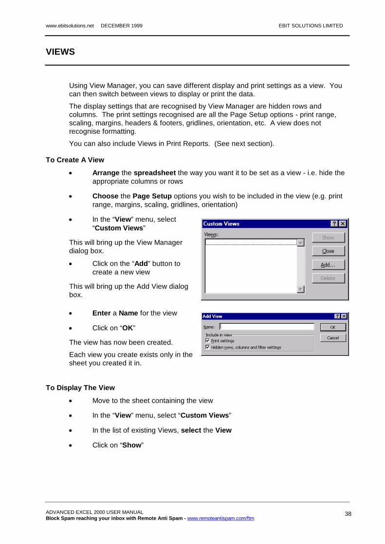
In the “View” menu, select “Custom Views”

This will bring up the View Manager dialog box.

Click on the “Add” button to create a new view

This will bring up the Add View dialog box.

Enter a Name for the view

Click on “OK”

The view has now been created.

Each view you create exists only in the sheet you created it in.

To Display The View

Move to the sheet containing the view

In the “View” menu, select “Custom Views”

In the list of existing Views, select the View

Click on “Show”



PRINT REPORTS

A Report is a collection of spreadsheet Scenarios and/or Views. Having specified the different Scenarios or Views you wish to be included in the report, you can print them all out in one go by printing the Report.

Print Reports are Workbook-specific, rather than sheet-specific.

You have to have installed the Report Manager ADD IN in order to create print reports

To Create A Print Report

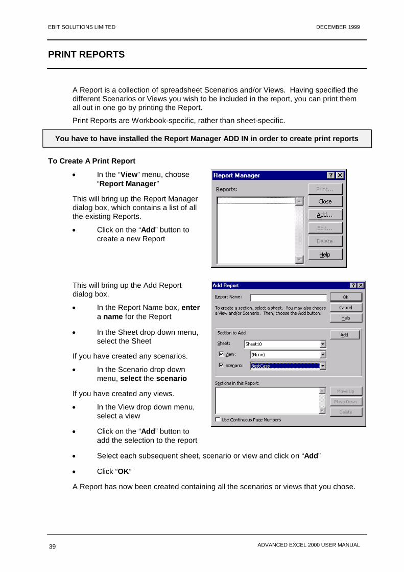
In the “View” menu, choose “Report Manager”

This will bring up the Report Manager dialog box, which contains a list of all the existing Reports.

Click on the “Add” button to create a new Report

This will bring up the Add Report dialog box.

In the Report Name box, enter a name for the Report

In the Sheet drop down menu, select the Sheet

If you have created any scenarios.

In the Scenario drop down menu, select the scenario

If you have created any views.

In the View drop down menu, select a view

Click on the “Add” button to add the selection to the report

Select each subsequent sheet, scenario or view and click on “Add”

Click “OK”

A Report has now been created containing all the scenarios or views that you chose.



40

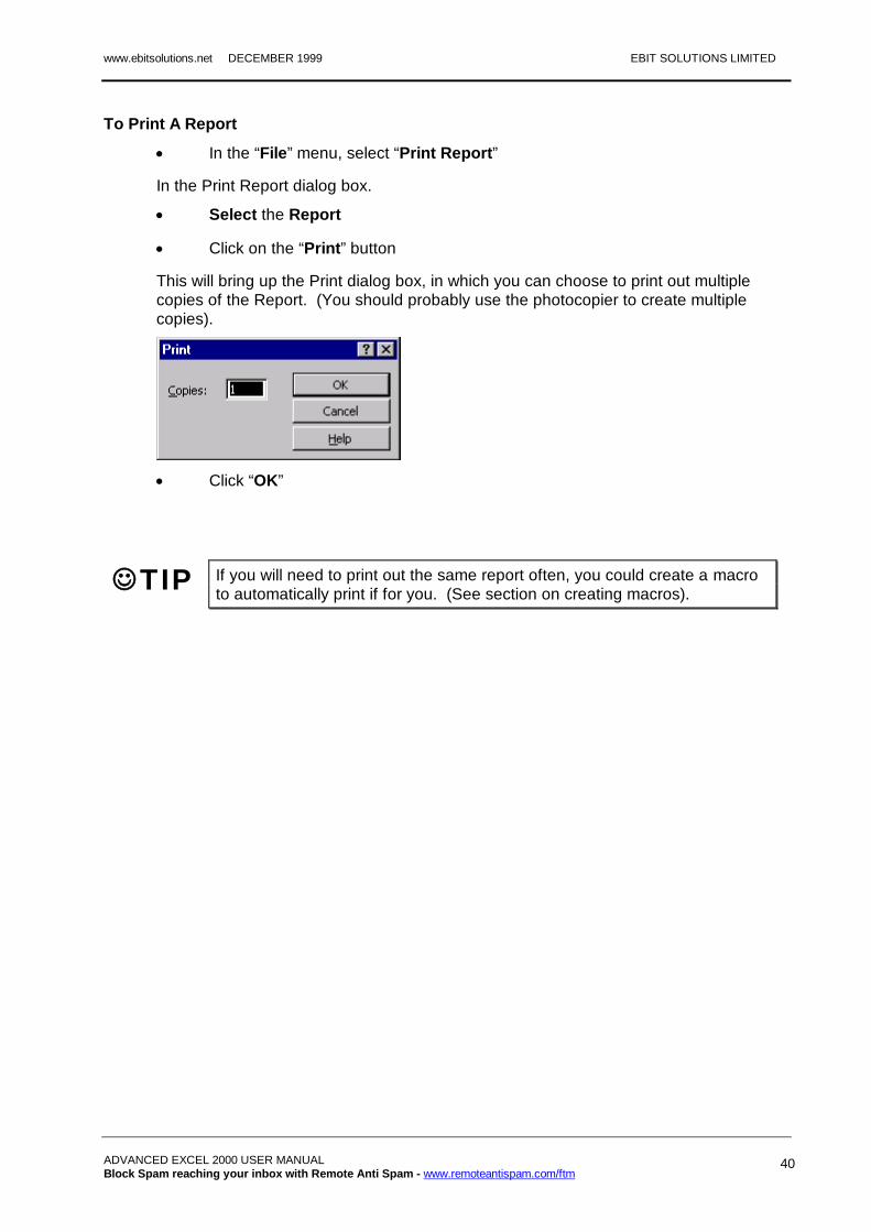
To Print A Report

In the “File” menu, select “Print Report”

In the Print Report dialog box.

Select the Report

Click on the “Print” button

This will bring up the Print dialog box, in which you can choose to print out multiple copies of the Report. (You should probably use the photocopier to create multiple copies).

Click “OK”

TIP If you will need to print out the same report often, you could create a macro to automatically print if for you. (See section on creating macros).



PIVOT TABLES AND PIVOT CHARTS

A pivot table and Pivot Chart is an interactive spreadsheet table or chart used to summarise and analyse data from an existing table of data.

Pivot Tables and charts are created using the Pivot Table and Pivotchart Wizard - a series of dialog boxes that guide you through the steps of specifying which data is to be used, and how it is to be analysed and displayed.

You can update (refresh) a pivot table or chart whenever changes occur in the original source data.

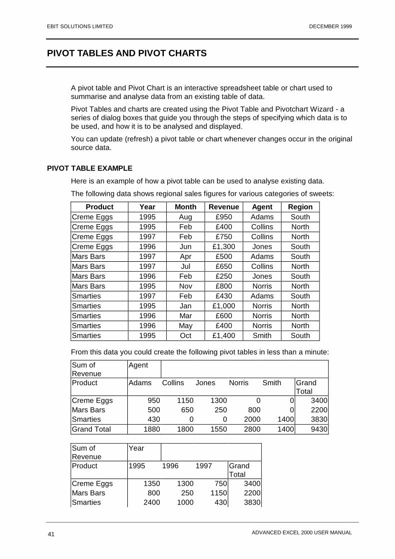
PIVOT TABLE EXAMPLE

Here is an example of how a pivot table can be used to analyse existing data.

The following data shows regional sales figures for various categories of sweets:

Product Year Month Revenue Agent Region Creme Eggs 1995 Aug £950 Adams South Creme Eggs 1995 Feb £400 Collins North Creme Eggs 1997 Feb £750 Collins North Creme Eggs 1996 Jun £1,300 Jones South Mars Bars 1997 Apr £500 Adams South Mars Bars 1997 Jul £650 Collins North Mars Bars 1996 Feb £250 Jones South Mars Bars 1995 Nov £800 Norris North Smarties 1997 Feb £430 Adams South Smarties 1995 Jan £1,000 Norris North Smarties 1996 Mar £600 Norris North Smarties 1996 May £400 Norris North Smarties 1995 Oct £1,400 Smith South

From this data you could create the following pivot tables in less than a minute:

Sum of Revenue

Agent

Product Adams Collins Jones Norris Smith Grand Total

Creme Eggs 950 1150 1300 0 0 3400 Mars Bars 500 650 250 800 0 2200 Smarties 430 0 0 2000 1400 3830 Grand Total 1880 1800 1550 2800 1400 9430 Sum of Revenue

Year

Product 1995 1996 1997 Grand Total

Creme Eggs 1350 1300 750 3400 Mars Bars 800 250 1150 2200 Smarties 2400 1000 430 3830



42

Grand Total 4550 2550 2330 9430

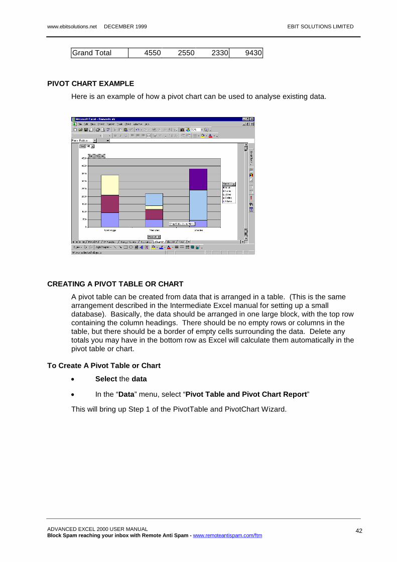
PIVOT CHART EXAMPLE

Here is an example of how a pivot chart can be used to analyse existing data.

CREATING A PIVOT TABLE OR CHART

A pivot table can be created from data that is arranged in a table. (This is the same arrangement described in the Intermediate Excel manual for setting up a small database). Basically, the data should be arranged in one large block, with the top row containing the column headings. There should be no empty rows or columns in the table, but there should be a border of empty cells surrounding the data. Delete any totals you may have in the bottom row as Excel will calculate them automatically in the pivot table or chart.

To Create A Pivot Table or Chart

Select the data

In the “Data” menu, select “Pivot Table and Pivot Chart Report”

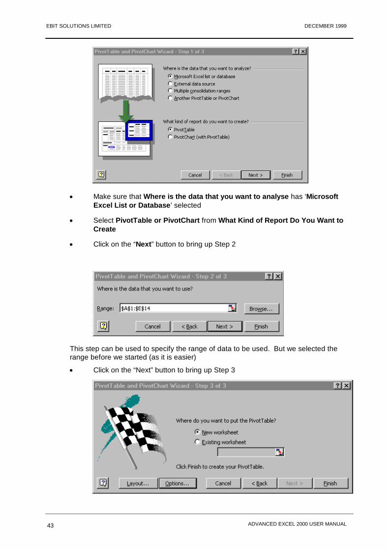
This will bring up Step 1 of the PivotTable and PivotChart Wizard.



Make sure that Where is the data that you want to analyse has ‘Microsoft Excel List or Database’ selected

Select PivotTable or PivotChart from What Kind of Report Do You Want to Create

Click on the “Next” button to bring up Step 2

This step can be used to specify the range of data to be used. But we selected the range before we started (as it is easier)

Click on the “Next” button to bring up Step 3



44

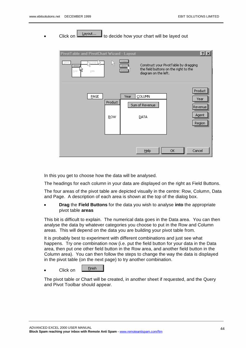
Click on to decide how your chart will be layed out

In this you get to choose how the data will be analysed.

The headings for each column in your data are displayed on the right as Field Buttons.

The four areas of the pivot table are depicted visually in the centre: Row, Column, Data and Page. A description of each area is shown at the top of the dialog box.

Drag the Field Buttons for the data you wish to analyse into the appropriate pivot table areas

This bit is difficult to explain. The numerical data goes in the Data area. You can then analyse the data by whatever categories you choose to put in the Row and Column areas. This will depend on the data you are building your pivot table from.

It is probably best to experiment with different combinations and just see what happens. Try one combination now (i.e. put the field button for your data in the Data area, then put one other field button in the Row area, and another field button in the Column area). You can then follow the steps to change the way the data is displayed in the pivot table (on the next page) to try another combination.

Click on

The pivot table or Chart will be created, in another sheet if requested, and the Query and Pivot Toolbar should appear.



To Change The Way The Data Is Displayed In The Pivot Table

Click in the pivot table

Click on the “PivotTable and PivotChart Wizard” button

then

or (if the Query and Pivot toolbar is not visible)

In the “View” menu, select “Toolbars” then Pivot Table

This will bring up the PivotTable and PivotChart Wizard.

To Update The Pivot Table

If you change the data that the pivot table is based on, you will need to update the pivot table to reflect the latest changes.

Click in the pivot table

Click on the “Refresh Data” button

or (if the Query and Pivot toolbar is not visible)

In the “Data” menu, select “Refresh Data”

To Delete A Pivot Table

Select the pivot table

In the “Edit” menu, choose “Clear”, then “All”



46



USER-DEFINED CHART FORMATS

If you need to create the same type of chart regularly, but find you are spending time formatting the chart each time you create it, you can set up your own ‘user-defined’ chart format. You can then create a new chart based on this format at any time.

To Create Your Own Chart Format

Create a new chart and format it the way you wish all your charts to look, or find a chart you created earlier in this format

Right click on the chart

Select "Chart Type”

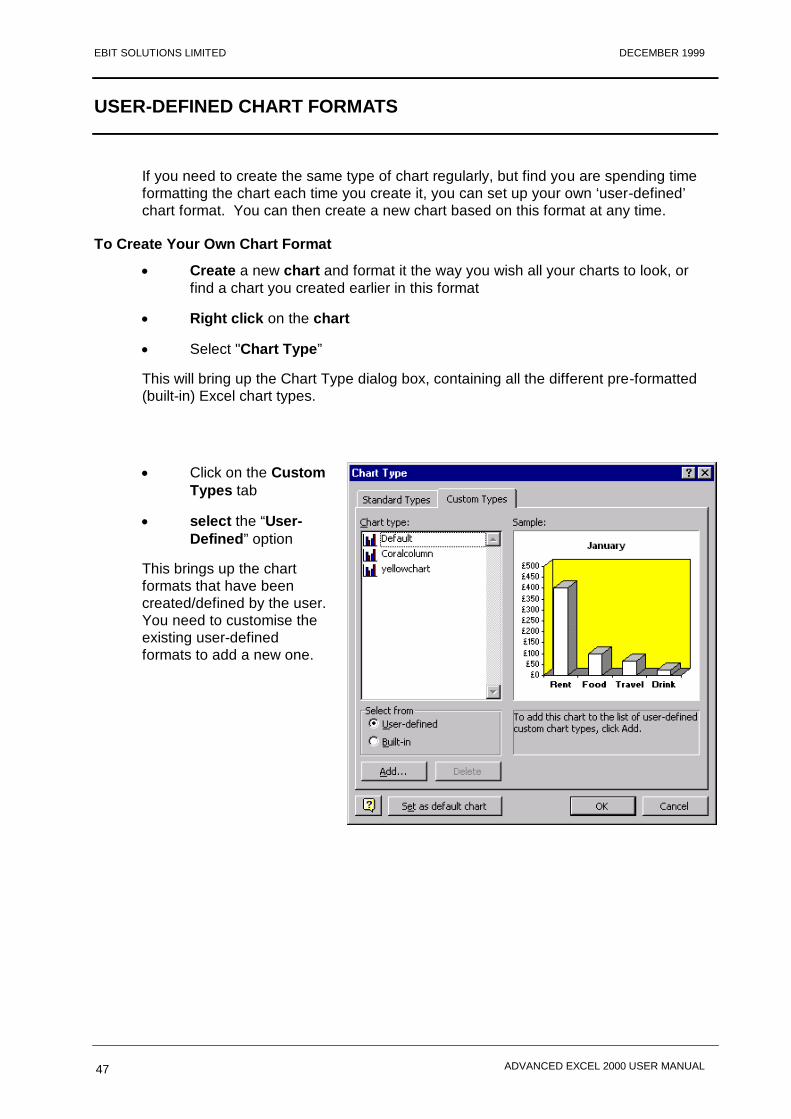
This will bring up the Chart Type dialog box, containing all the different pre-formatted (built-in) Excel chart types.

Click on the Custom Types tab

select the “User-Defined” option

This brings up the chart formats that have been created/defined by the user. You need to customise the existing user-defined formats to add a new one.



48

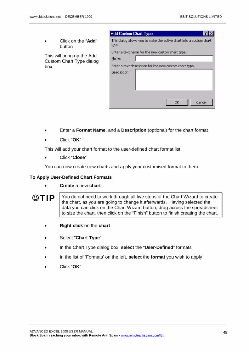
Click on the “Add” button

This will bring up the Add Custom Chart Type dialog box.

Enter a Format Name, and a Description (optional) for the chart format

Click “OK”

This will add your chart format to the user-defined chart format list.

Click “Close”

You can now create new charts and apply your customised format to them.

To Apply User-Defined Chart Formats

Create a new chart

TIP You do not need to work through all five steps of the Chart Wizard to create the chart, as you are going to change it afterwards. Having selected the data you can click on the Chart Wizard button, drag across the spreadsheet to size the chart, then click on the “Finish” button to finish creating the chart.

Right click on the chart

Select "Chart Type"

In the Chart Type dialog box, select the “User-Defined” formats

In the list of ‘Formats’ on the left, select the format you wish to apply

Click “OK”



PROTECTING SHEETS AND WORKBOOKS

If you have created a spreadsheet that you do not want to be altered by the other people that might view it, you can protect the sheet. You can either protect the whole sheet, or just certain key cells in the sheet (probably those containing the formulas) so that new data can still be entered onto the sheet.

You can also protect a whole workbook. Workbook protection on its own, stops the user from inserting new sheets or deleting sheets, but not from editing cell contents. To do this you should protect the workbook and also protect every sheet in it.

To Protect A Whole Sheet

Select the sheet you wish to protect

In the “Tools” menu, select “Protection”, then “Protect Sheet”

This will bring up the Protect Sheet dialog box, in which you can enter a password to prevent users from unprotecting the sheet. But you do not have to use a password. You can just leave the Password box empty.

Warning - Do not use a password unless you are certain that you won’t forget what it is.

Passwords are case sensitive.

Enter a password (only if necessary)

Click “OK”

If you have entered a password, you will be asked to confirm the password.

Type in the password again

The whole sheet is now protected. Users will not be able to change the contents of any cell. If you need to change cell contents you will need to unprotect the sheet.



50

To Unprotect A Sheet

Select the sheet you wish to unprotect

In the “Tools” menu, select “Protection”, then “Unprotect Sheet”

If no password was originally used to protect the sheet, then the sheet will automatically be unprotected at this point.

If a password has been used, the Unprotect Sheet dialog box will appear.

Enter the password

Click on “OK”

The sheet will now be unprotected

LOCKING AND UNLOCKING CELLS

By default, every cell in a sheet has ‘locking’ applied to it. It is the locking that is activated when the sheet is protected and stops people from editing cells.

If you want to protect part of a sheet (perhaps containing the formulas), but leave other cells open so that users can enter new data, you will need to ‘unlock’ the cells that will be changed at a later date.

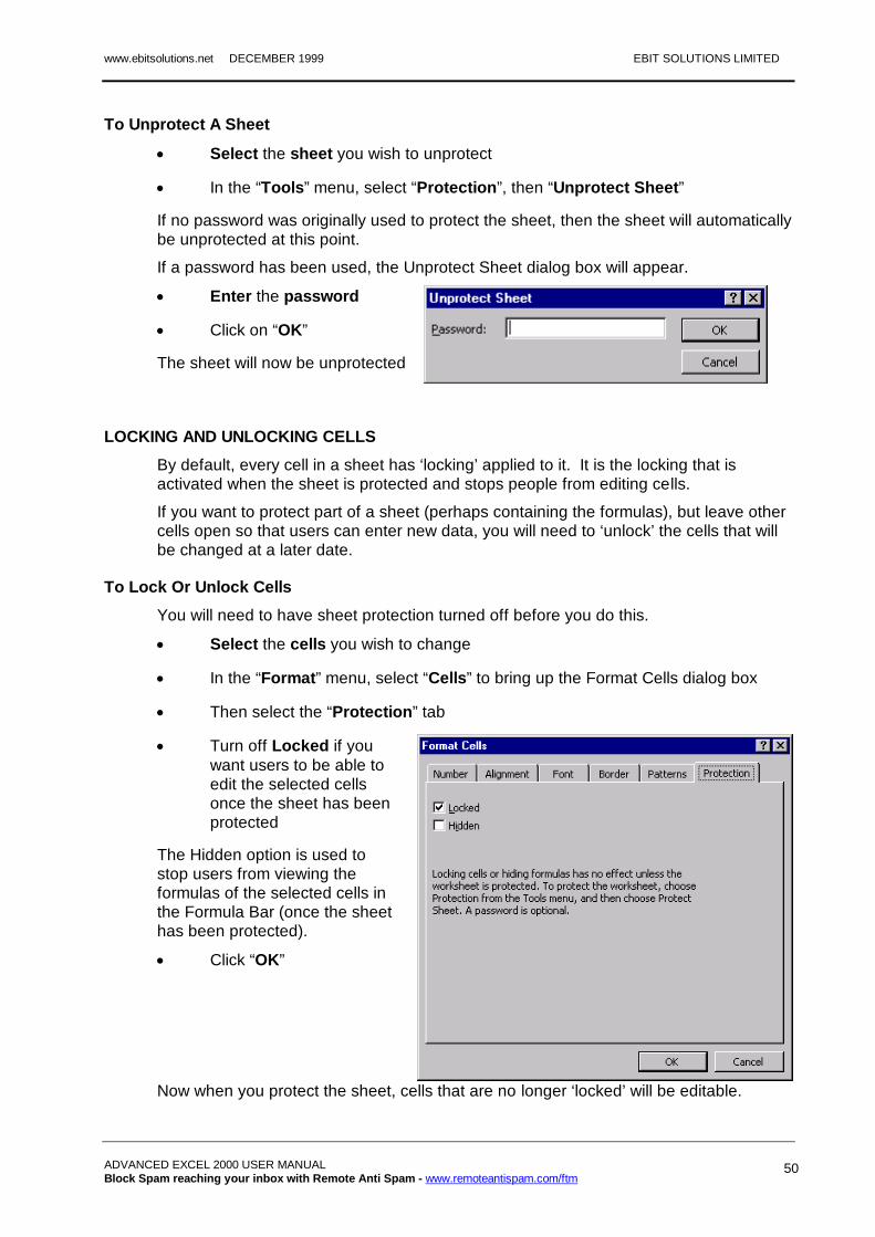
To Lock Or Unlock Cells

You will need to have sheet protection turned off before you do this.

Select the cells you wish to change

In the “Format” menu, select “Cells” to bring up the Format Cells dialog box

Then select the “Protection” tab

Turn off Locked if you want users to be able to edit the selected cells once the sheet has been protected

The Hidden option is used to stop users from viewing the formulas of the selected cells in the Formula Bar (once the sheet has been protected).

Click “OK”

Now when you protect the sheet, cells that are no longer ‘locked’ will be editable.



52

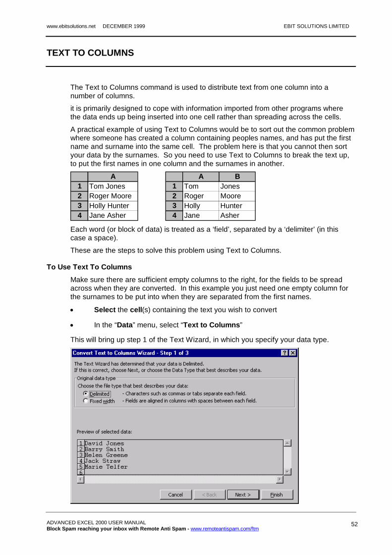
TEXT TO COLUMNS

The Text to Columns command is used to distribute text from one column into a number of columns.

it is primarily designed to cope with information imported from other programs where the data ends up being inserted into one cell rather than spreading across the cells.

A practical example of using Text to Columns would be to sort out the common problem where someone has created a column containing peoples names, and has put the first name and surname into the same cell. The problem here is that you cannot then sort your data by the surnames. So you need to use Text to Columns to break the text up, to put the first names in one column and the surnames in another.

A1 Tom Jones2 Roger Moore3 Holly Hunter4 Jane Asher

A B1 Tom Jones2 Roger Moore3 Holly Hunter4 Jane Asher

Each word (or block of data) is treated as a ‘field’, separated by a ‘delimiter’ (in this case a space).

These are the steps to solve this problem using Text to Columns.

To Use Text To Columns

Make sure there are sufficient empty columns to the right, for the fields to be spread across when they are converted. In this example you just need one empty column for the surnames to be put into when they are separated from the first names.

Select the cell(s) containing the text you wish to convert

In the “Data” menu, select “Text to Columns”

This will bring up step 1 of the Text Wizard, in which you specify your data type.



Delimited: is used when the data has a character separating each field, such as a space (as we have here) or a tab.

Fixed Width: is used when, for example, someone has put in lots of spaces or tabs to line the fields up in columns.

Specify your Data Type by selecting Delimited or Fixed Width as appropriate

In this example select Delimited.

Click on “Next”

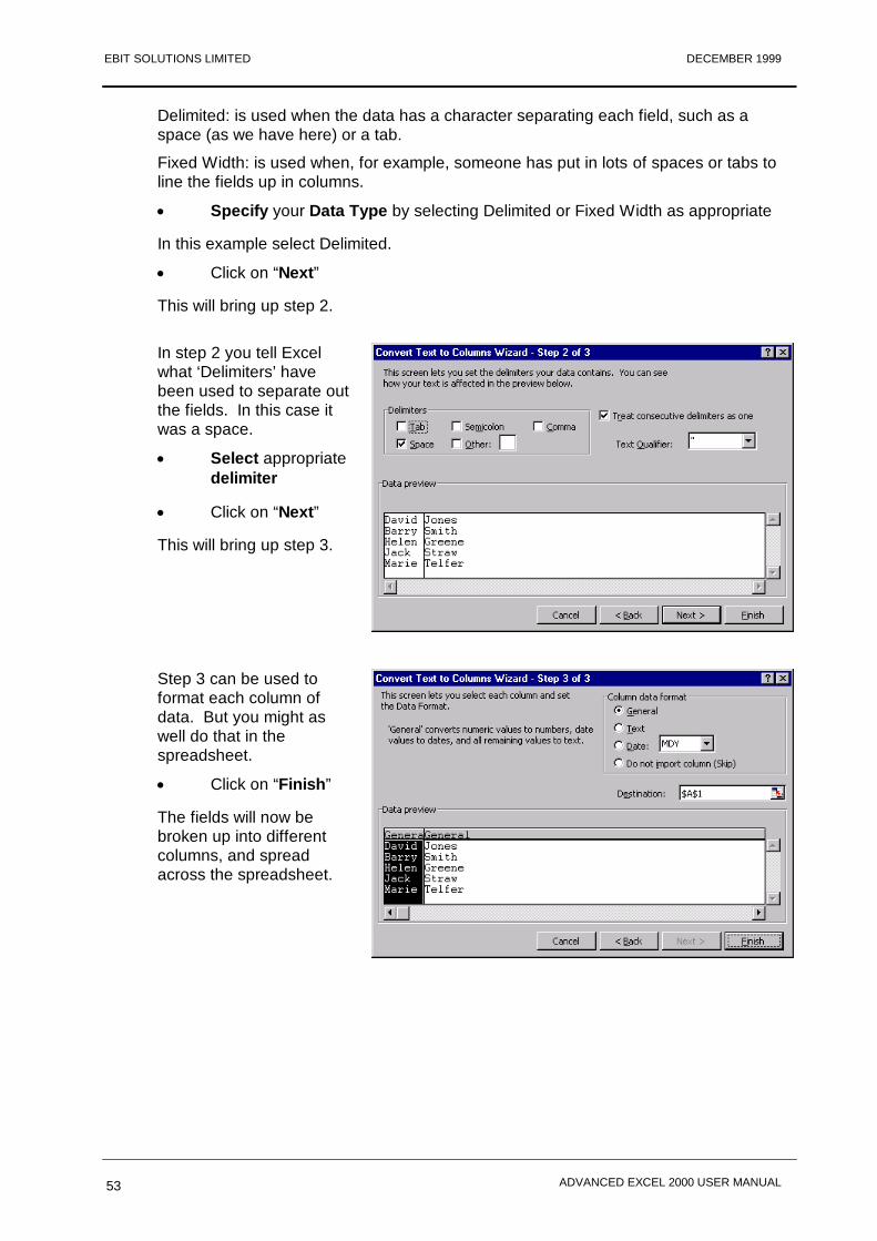
This will bring up step 2.

In step 2 you tell Excel what ‘Delimiters’ have been used to separate out the fields. In this case it was a space.

Select appropriate delimiter

Click on “Next”

This will bring up step 3.

Step 3 can be used to format each column of data. But you might as well do that in the spreadsheet.

Click on “Finish”

The fields will now be broken up into different columns, and spread across the spreadsheet.



54

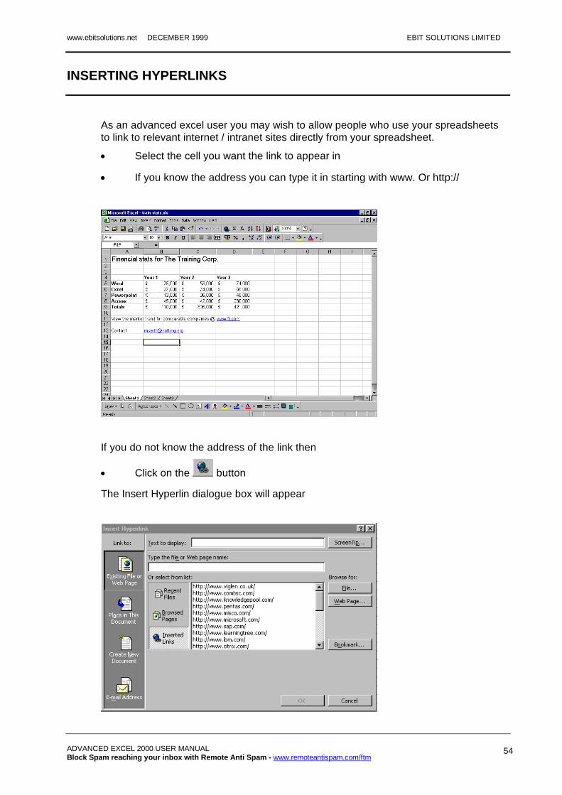
INSERTING HYPERLINKS

As an advanced excel user you may wish to allow people who use your spreadsheets to link to relevant internet / intranet sites directly from your spreadsheet.

Select the cell you want the link to appear in

If you know the address you can type it in starting with www. Or http://

If you do not know the address of the link then

Click on the button

The Insert Hyperlin dialogue box will appear



You can select a link from the Inserted Links shown or you can click on to browse the internet for the site of your choice.

Once you have got the site of your choice you should swich back to Excel 2000 and the correct link will appear in the Type the File or Web Page Name Field:.

Click on to insert the link.

The link will appear underlined in blue by default and once clicked on will change colour.

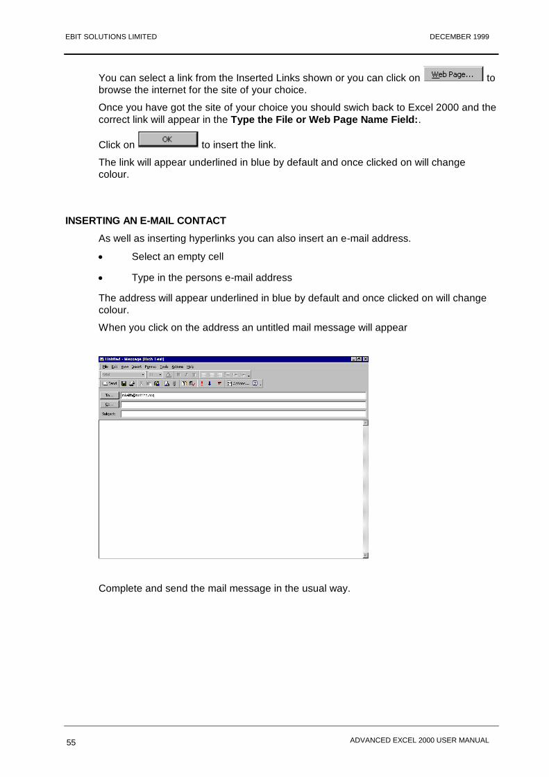
INSERTING AN E-MAIL CONTACT

As well as inserting hyperlinks you can also insert an e-mail address.

Select an empty cell

Type in the persons e-mail address

The address will appear underlined in blue by default and once clicked on will change colour.

When you click on the address an untitled mail message will appear

Complete and send the mail message in the usual way.

15682845 advanced excel 2000 user guide

Documents