1

DISTRIBUTION STATEMENT A. Approved for public release; distribution is unlimited.

Inner Shelf DRI: The Interaction of Surf Zone and Inner Shelf Flows &

Spatial and Temporal Observations of Wind Stress along a Sandy Beach & includes results from

New River Inlet DRI: Observations and Modeling of Flow and Material Exchange &

Field and Numerical Study of the Columbia River Mouth

Jamie MacMahan Oceanography Department, Spanagel 327c, Naval Postgraduate School

Monterey, CA 93943 Phone: (831) 656-2379 Fax: (831) 656-2712 Email: jhmacmah@nps.edu

NPS Award Number: (PTSAL: N0001415WX00574, N0001415WX00895; Wind Stress:

N0001415WX01719; RIVET: N0001411WX20962; N0001412WX20498)

Ad Reniers Rosenstiel School of Marine and Atmospheric Science

Miami, FL33149 Phone: (305) 421-4223 Fax: (305) 421-4701 Email: areniers@rsmas.miami.edu

UM Award Number: (N000141010409, N000141010379)

LONG-TERM GOALS 1) To understand, measure and model the wave, flow and temperature variability within the inner

shelf over a wide range of temporal and spatial scales.

2) To quantify the temporal and spatial variability of the wind stress along a sandy beach in Monterey, CA that is hypothesized to vary owing to wave height, wave direction, shoreline orientation, and land topography based on the results by Ortiz-Suslow et al. (2014) and Shebani et al. (2013).

OBJECTIVES The main objectives of our FY15 effort were to: • obtain in situ observations of temperature, pressure, and velocity at Point Sal, CA, as part of the

pilot effort inner shelf DRI;

• analyze inner shelf observations exploring subtidal, tidal, solitons, and surfzone influences on temperature structure;

• obtain and analyze subaerial momentum flux observations at the high-tide line on a sandy beach

• purchase and construct portable wind stress stations for evaluating land-sea interactions along the coast

2

• continue analysis of New River Inlet (NRI) water characterization with Ad Reniers and Patrick Rynne;

• continue analysis of MCR observations with Ad Reniers, Guy Gelfenbaum, and Andrew Stevens

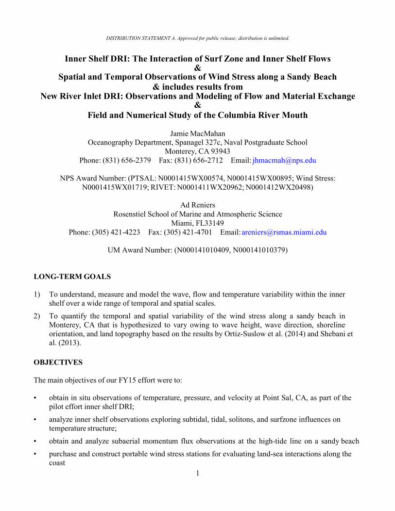
APPROACH Field experiments were designed and performed to meet the above objectives using equipment obtained with ONR DURIP funding. WORK COMPLETED We (MacMahan, NPS students (Thomas Friesmuth, Colleen McDonald, Mathias Roth, and Darin Keeter) and technicians (Keith Wyckoff)) deployed 29 temperature stations and 6 ADCP sea spider tripods in the inner shelf off Point Sal, CA in June and July 2015 (Figure 1). The experimental design focused on describing the spatial, including the vertical, and temporal scales of temperature variability for the inner shelf induced by offshore process (e.g., subtidal flows, internal tidal bores, and solitons) and surf zone processes (e.g., rip currents) that were additionally modified by the presence of rocky points and a large offshore subaqueous rocky outcrop. In total, 286 temperature sensors, 6 ADCPs, 12 pressure sensors, and 29 tilt sensors were deployed and successfully recovered. All sensors collected observations continuously at 1 Hz for 43 days. The instrument locations were determined though model simulations using ROMs from the DRI modeling group consisting of scientists from SCRIPPs and Georgia Tech. We have begun analyzing the data and are collaborating with John Colosi at NPS and Joe Calantoni at NRL. This data will be used for Thomas’s NPS PhD dissertation.

Figure 1. Map of experiment site near Pt. Sal, CA. Blue dots indicate locations of thermistor

strings (TS) and red squares indicate locations of ADCPs. Bathymetry (shading) data used in this study were acquired, processed, archived, and distributed by the Seafloor Mapping Lab of California State University Monterey Bay. X, Yi, Yo, PS, and PSB represent cross-shore

array, alongshore inner array, alongshore outer array, Point Sal array, and Point Sal Beach array, respectively.

3

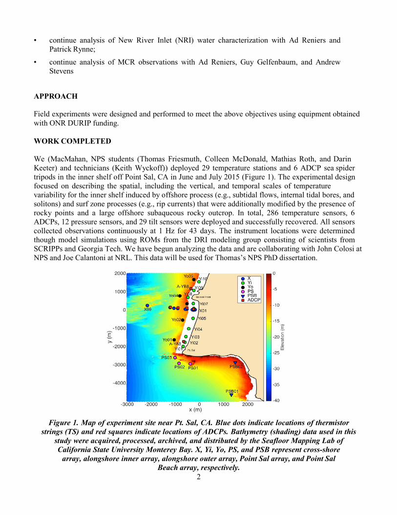
We (MacMahan and student Darin Keeter) purchased and constructed momentum flux tower for measuring wind stress and local energy balance. The system was deployed within the inter-tidal zone at a sandy beach in Monterey CA between March 2015 and July 2015. This resulted in the collection of 111 days of temperature and momentum flux data at 1, 3 and 6m elevations over 4 separate deployment periods. The flux tower used Campbell Scientific data logger for data integration and high sampling frequency of the sonic anemometers. Tower sensors included two sonic anemometers, two temperature and humidity sensors, a downward-looking infrared radiometer and net radiometer to measure total solar and terrestrial radiation. In conjunction with the tower flux, additional sensors were deployed such as offshore water temperature sensors and pressure sensors. Additional data were also gathered from the fixed met sensors at the Del Monte beach laboratory, approximately 100 m from the experiment site, tidal data from the NOAA tidal station in Monterey harbor and periodic GPS beach profiles were taken to ascertain the actual water level on the beach. Programs were developed for QCing and rotating the sonic anemometer data (Aubinet et al., 2012). Data are currently being analyzed as part of Darin’s NPS MS thesis. RESULTS Observations of Oceanic-Forced Subtidal Elevations in a Convergent Estuary Remotely-forced downwelling events are found to generate oceanic subtidal elevations along the Pacific Northwest that were transmitted into estuaries and upstream in a large, river-tide, convergent estuary, Columbia River estuary (CRE). The subtidal generation mechanisms were evaluated using NOAA tidal and USGS river gage station data along the northern California, Oregon, and Washington estuaries and throughout the Columbia River and the NOAA Coastal Upwelling Index (CUI). River discharge pulses generate subtidal motions that propagate downstream with decreasing amplitude. Oceanic downwelling-induced subtidal motions propagate upstream with a slight decrease in amplitude. The oceanic subtidal motions represent 90% of the total subtidal contribution and decrease to 40% upstream. Hourly water level elevations were obtained from the NOAA-NOS tidal stations located in estuaries along the west coast from northern California to northern Washington for 2013 and throughout the CRE (http://tidesandcurrents.noaa.gov). Gage height elevations were obtained from the USGS Bonneville Dam. The analysis initially focuses on using one-year of data that allows a qualitative examination of the time series to describe the physical processes relevant to subtidal motions, which are then quantitatively analyzed using 21 years. The year 2013 is selected for the one- year analysis to provide background information for evaluating the effect of subtidal motions for subsequent papers describing an Office of Naval Research field experiment at the MCR (RIVET-II) conducted in 2013. In addition, 21-year records of water level elevations are selected for Astoria, Toke Point and Bonneville Dam stations for long-term analysis. A Coastal Upwelling Index, CUI, describes the cross-shelf transport of water transport in the Ekman Layer forced by wind stress (Ekman, 1905) on the west coast of the North America is computed by NOAA [http://www.pfeg.noaa.gov/products/PFEL/modeled/indices/upwelling/upwelling.html]. Positive CUI values indicate offshore transport associated with coastal upwelling, and negative values indicate onshore transport associated with coastal downwelling. The NOAA-NOS tidal elevations for 2013 were low-passed filtered with a frequency cut-off of 1/2 d-1

representing the subtidal variation (Figure 2). There were O(0.5m) subtidal elevations that episodically occur at all stations along the coast. The magnitude and duration varies along the coast. The largest subtidal elevations occur at AS (Astoria, OR), TP (Toke Point, WA), and LP (La Push,

4

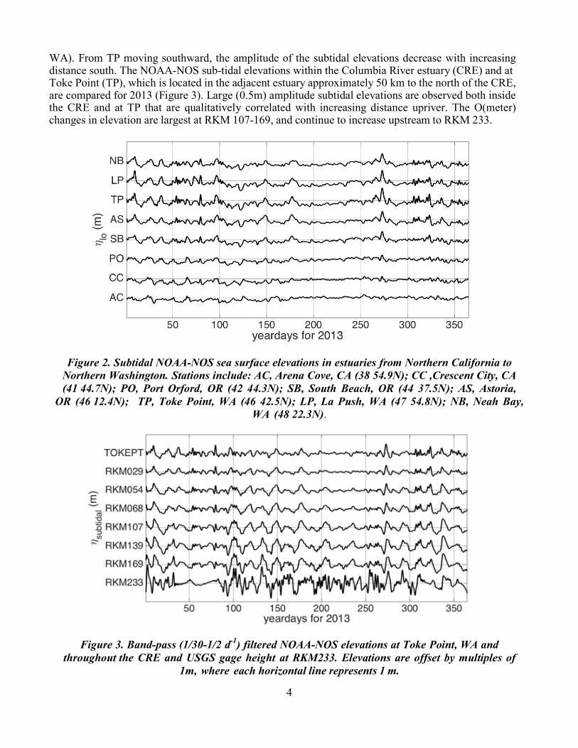
WA). From TP moving southward, the amplitude of the subtidal elevations decrease with increasing distance south. The NOAA-NOS sub-tidal elevations within the Columbia River estuary (CRE) and at Toke Point (TP), which is located in the adjacent estuary approximately 50 km to the north of the CRE, are compared for 2013 (Figure 3). Large (0.5m) amplitude subtidal elevations are observed both inside the CRE and at TP that are qualitatively correlated with increasing distance upriver. The O(meter) changes in elevation are largest at RKM 107-169, and continue to increase upstream to RKM 233.

Figure 2. Subtidal NOAA-NOS sea surface elevations in estuaries from Northern California to Northern Washington. Stations include: AC, Arena Cove, CA (38 54.9N); CC ,Crescent City, CA (41 44.7N); PO, Port Orford, OR (42 44.3N); SB, South Beach, OR (44 37.5N); AS, Astoria,

OR (46 12.4N); TP, Toke Point, WA (46 42.5N); LP, La Push, WA (47 54.8N); NB, Neah Bay, WA (48 22.3N).

Figure 3. Band-pass (1/30-1/2 d-1) filtered NOAA-NOS elevations at Toke Point, WA and

throughout the CRE and USGS gage height at RKM233. Elevations are offset by multiples of 1m, where each horizontal line represents 1 m.

5

Hypothesis 1 is that the subtidal motions within estuary are generated by the temporal variations in the spring-neap tidal modulation (LeBlond, 1978, 1979; Jay and Flinchem 1997; Godin and Martinez, 1994; Godin, 1999; Buschman et al., 2009). The upper tidal elevation envelope (Apos) representing the spring-neap modulation is computed from the low-pass (1/2 d-1) Hilbert transform (H) of the positive tidal elevations (ηpos(t)), as defined by (Melville, 1983). Apos(t) and ηpos(t) are computed for the observed tidal elevations at Astoria, RMK 29. The yearly-averaged cross-correlation using 21 years of observations between Apos(t) and ηpos(t) has a maximum r-value of 0.53 with minimal temporal lag and is significantly correlated at the 95% significance level (purple line, Figure 4). Hypothesis 2 is that subtidal pulses in the river discharge generate the subtidal motions. The cross-correlation function for sea surface elevations between RKM233 and RKM29 results in a maximum r-value of 0.22 (red line, Figure 4). Though significantly correlated, the negative temporal lag suggests that subtidal motions at the river mouth are ahead of river discharge pulses. Therefore, this is a not a valid mechanism for subtidal generation near the river mouth. Hypothesis 3 is that the downwelling-events induce a sea surface elevation at the river mouth that is transmitted into the estuary (Garvine, 1985). The correlation function between the CUI and sea surface elevation at Astoria is negatively correlated with a minimum r-value of -0.52 with a 2-day temporal lag, which is significant at 95% (blue line, Figure 4). Two days after the downwelling event occurs, a coastal set-up of sea surface elevation arrives at Astoria inside the estuary. It is not clear as to why there is a two day lag in the development of the coastal set-up that is observed at Astoria. All hypotheses appear valid based on correlation results in suggesting that there are concomitant mechanisms for generating subtidal pulses that propagate upstream and downstream. Qualitatively, Hypothesis 3 appears valid for generation of upstream subtidal pulses.

Figure 4. Cross-correlation functions for sea surface elevations, CUI, and spring-neap modulations over 21 years. The dashed black lines represent the 95% significance level. Positive lag

represents that the time series at the corresponding station leads.

6

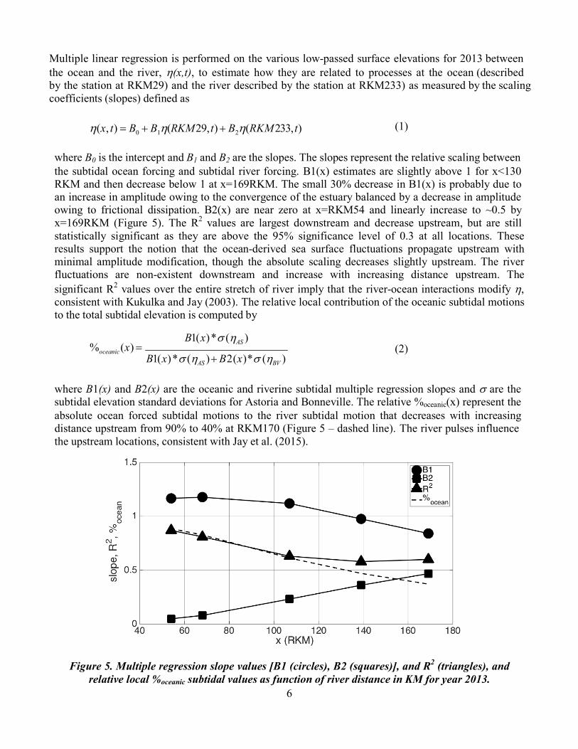
Multiple linear regression is performed on the various low-passed surface elevations for 2013 between the ocean and the river, η(x,t), to estimate how they are related to processes at the ocean (described by the station at RKM29) and the river described by the station at RKM233) as measured by the scaling coefficients (slopes) defined as

η(x, t) = B0 + B1η(RKM 29, t) + B2η(RKM 233, t)

(1)

where B0 is the intercept and B1 and B2 are the slopes. The slopes represent the relative scaling between the subtidal ocean forcing and subtidal river forcing. B1(x) estimates are slightly above 1 for x<130 RKM and then decrease below 1 at x=169RKM. The small 30% decrease in B1(x) is probably due to an increase in amplitude owing to the convergence of the estuary balanced by a decrease in amplitude owing to frictional dissipation. B2(x) are near zero at x=RKM54 and linearly increase to ~0.5 by x=169RKM (Figure 5). The R2 values are largest downstream and decrease upstream, but are still statistically significant as they are above the 95% significance level of 0.3 at all locations. These results support the notion that the ocean-derived sea surface fluctuations propagate upstream with minimal amplitude modification, though the absolute scaling decreases slightly upstream. The river fluctuations are non-existent downstream and increase with increasing distance upstream. The significant R2 values over the entire stretch of river imply that the river-ocean interactions modify η, consistent with Kukulka and Jay (2003). The relative local contribution of the oceanic subtidal motions to the total subtidal elevation is computed by

B1(x)*σ (ηAS ) %oceanic (x) =

B1(x)*σ (ηAS ) + B2(x)*σ (ηBV ) (2)

where B1(x) and B2(x) are the oceanic and riverine subtidal multiple regression slopes and σ are the subtidal elevation standard deviations for Astoria and Bonneville. The relative %oceanic(x) represent the absolute ocean forced subtidal motions to the river subtidal motion that decreases with increasing distance upstream from 90% to 40% at RKM170 (Figure 5 – dashed line). The river pulses influence the upstream locations, consistent with Jay et al. (2015).

Figure 5. Multiple regression slope values [B1 (circles), B2 (squares)], and R2 (triangles), and relative local %oceanic subtidal values as function of river distance in KM for year 2013.

7

r

Tidal exchange at New River Inlet The mean residence time (T ) in a single inlet system is a function of tidal exchange through the relationship defined as

T V T = r

ocean lagoon (3)

where T is the tidal period, V is the volume of the embayment, P is the tidal prism volume, and ε

ocean and ε lagoon

are tidal exchange fractions that describe what percentage of the tidal prism volume is replaced on each ebb and flood respectively (Rynne et al 2015). Despite improved methods to predict tidal exchange, little attention has been placed on its temporal variability from one tidal cycle to the next or the nearshore processes that affect it.

Figure 6. The extent of the ebb flow is shown for both maximum (top) and minimum

(bottom) ocean exchange. The ocean exchange fraction varies with the direction and magnitude of alongshore currents. Maximum exchange is achieved when ebbing waters are drawn far

away from the inlet mouth. Minimum exchange occurs when ebbing water remains close to the inlet mouth.

ε ε P

8

Flow, pressure, and dye concentration observations from the RIVET I experiment at New River Inlet are used to calibrate and validate a coupled Delft3D-SWAN hydrodynamic and wave model. The calibrated model is then used to quantify tidal exchange fractions from May 1 – May 22, 2012 and determine which processes control its variability. The ocean exchange fraction is controlled by the development of alongshore currents through two mechanisms. Maximum ocean exchange (Figure 6, top) occurs when wave induced alongshore currents drive ebbing water far from the inlet mouth. Weaker southerly currents are thought to be driven by alongshore pressure gradients that are controlled by subtidal motions across the shelf (Raubenheimer, personal communication). Minimum ocean exchange occurs when conditions shift between these two mechanisms and the alongshore currents are weakest (Figure 7, middle). The lagoon exchange fraction is controlled by the tidal prism volume, which is further controlled by the semi-diurnal, diurnal, and subtidal fluctuations. Maximum lagoon exchange occurs during spring tides when the tidal prism is largest (Figure 7, top) and minimum lagoon exchange occurs during neap tides when the tidal prism is smallest (Figure 7, middle).

Figure 7. The extent of the flood flow is shown for both maximum (top) and minimum (bottom) lagoon exchange. The lagoon exchange fraction varies with the tidal prism volume following spring neap tidal fluctuations. Maximum exchange is achieved when the tidal prism is largest (top) and flooding waters can penetrate far into the backbay. Minimum exchange occurs when flooding waters

cannot reach far past the inlet channel (bottom).

9

Inner Shelf Temperature Variability Observations of inner shelf temperature variability off of Point Sal, CA show a wealth of complex temperature signatures that are associated with subtidal, tidal, solitons, and wave forcing. Owing to the complexity and non-stationarity of the signal, only a few aspects will be highlighted here in at this time. Cross-shore and alongshore arrays were deployed around Pt. Sal to evaluate the evolution of the temperature signals. An example of the raw temperature signal as function elevation is provided in Figure 8 for two stations located in the cross-shore array separated by 1km in cross-shore distance for yearday 181. Station X09 is located in 15m water and X03 is located in 9m water depth (Figure 1). For station X09, there are aperiodic warm temperature fronts (tidal bores) observed with non-linear solitons present within the warmer surface water (Figure 8 top). Some of the solitons occur from the surface and extend O(10m) below the surface. Additional solitons are observed underneath the warm water tidal bore. For station X03, the magnitude of the solitons has diminished (Figure 8 bottom). There is large-scale correlation (Figure 8) with tidal bores as they propagate into shallow water, but the tidal bore structure has evolved over this relatively short distance, which is believed related to the irregular bathymetry.

Figure 8. The raw 1Hz temperature variability over the vertical for station X09 (top) and station X03 (bottom) located in 15 and 9m water depth for yearday 181. The stations are separated by 1km

in the cross-shore.

10

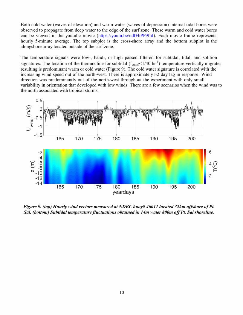
Both cold water (waves of elevation) and warm water (waves of depression) internal tidal bores were observed to propagate from deep water to the edge of the surf zone. These warm and cold water bores can be viewed in the youtube movie (https://youtu.be/ndfFbPF9fhI). Each movie frame represents hourly 5-minute average. The top subplot is the cross-shore array and the bottom subplot is the alongshore array located outside of the surf zone. The temperature signals were low-, band-, or high passed filtered for subtidal, tidal, and solition signatures. The location of the thermocline for subtidal (fcutoff<1/40 hr-1) temperature vertically migrates resulting is predominant warm or cold water (Figure 9). The cold water signature is correlated with the increasing wind speed out of the north-west. There is approximately1-2 day lag in response. Wind direction was predominantly out of the north-west throughout the experiment with only small variability in orientation that developed with low winds. There are a few scenarios when the wind was to the north associated with tropical storms.

Figure 9. (top) Hourly wind vectors measured at NDBC buoy# 46011 located 32km offshore of Pt. Sal. (bottom) Subtidal temperature fluctuations obtained in 14m water 800m off Pt. Sal shoreline.

11

Figure 10. (top) Raw temperature observations for station X08 for yearday 179. The white line represents the mean temperature isotherm. (middle) Band-passed temperature observations

estimated from the raw observations. (bottom) Contours of the Hilbert transform for upper envelopes of the band-passed temperature observation. Dashed lines represent arbitrary cut-off

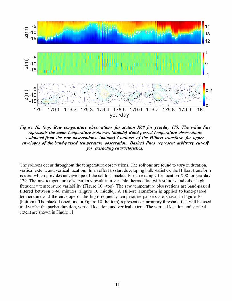
for extracting characteristics. The solitons occur throughout the temperature observations. The solitons are found to vary in duration, vertical extent, and vertical location. In an effort to start developing bulk statistics, the Hilbert transform is used which provides an envelope of the solitons packet. For an example for location X08 for yearday 179. The raw temperature observations result in a variable thermocline with solitons and other high frequency temperature variability (Figure 10 –top). The raw temperature observations are band-passed filtered between 5-60 minutes (Figure 10 middle). A Hilbert Transform is applied to band-passed temperature and the envelope of the high-frequency temperature packets are shown in Figure 10 (bottom). The black dashed line in Figure 10 (bottom) represents an arbitrary threshold that will be used to describe the packet duration, vertical location, and vertical extent. The vertical location and vertical extent are shown in Figure 11.

12

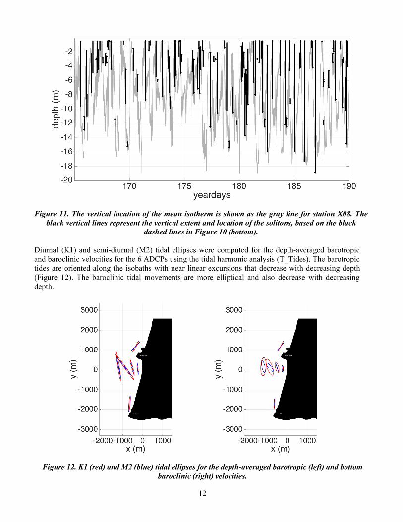
Figure 11. The vertical location of the mean isotherm is shown as the gray line for station X08. The black vertical lines represent the vertical extent and location of the solitons, based on the black

dashed lines in Figure 10 (bottom). Diurnal (K1) and semi-diurnal (M2) tidal ellipses were computed for the depth-averaged barotropic and baroclinic velocities for the 6 ADCPs using the tidal harmonic analysis (T_Tides). The barotropic tides are oriented along the isobaths with near linear excursions that decrease with decreasing depth (Figure 12). The baroclinic tidal movements are more elliptical and also decrease with decreasing depth.

Figure 12. K1 (red) and M2 (blue) tidal ellipses for the depth-averaged barotropic (left) and bottom baroclinic (right) velocities.

13

Sandy Beach Wind Stress Sonic anemometer data were collected near the high tide line for approximately 6 months. Owing to significant erosion and accretion that occurred during the experiment the tower had to be periodically moved and adjusted resulting in 4 deployment locations. In addition, the sensors were adjusted over the vertical to obtain different measures above the beach. The total wind shear velocity was computed directly using the eddy covariance techniques every 15 minutes, as defined as

𝜏 = −𝜌!(𝑢𝑤𝑖 + 𝑣𝑤𝑗), (4)

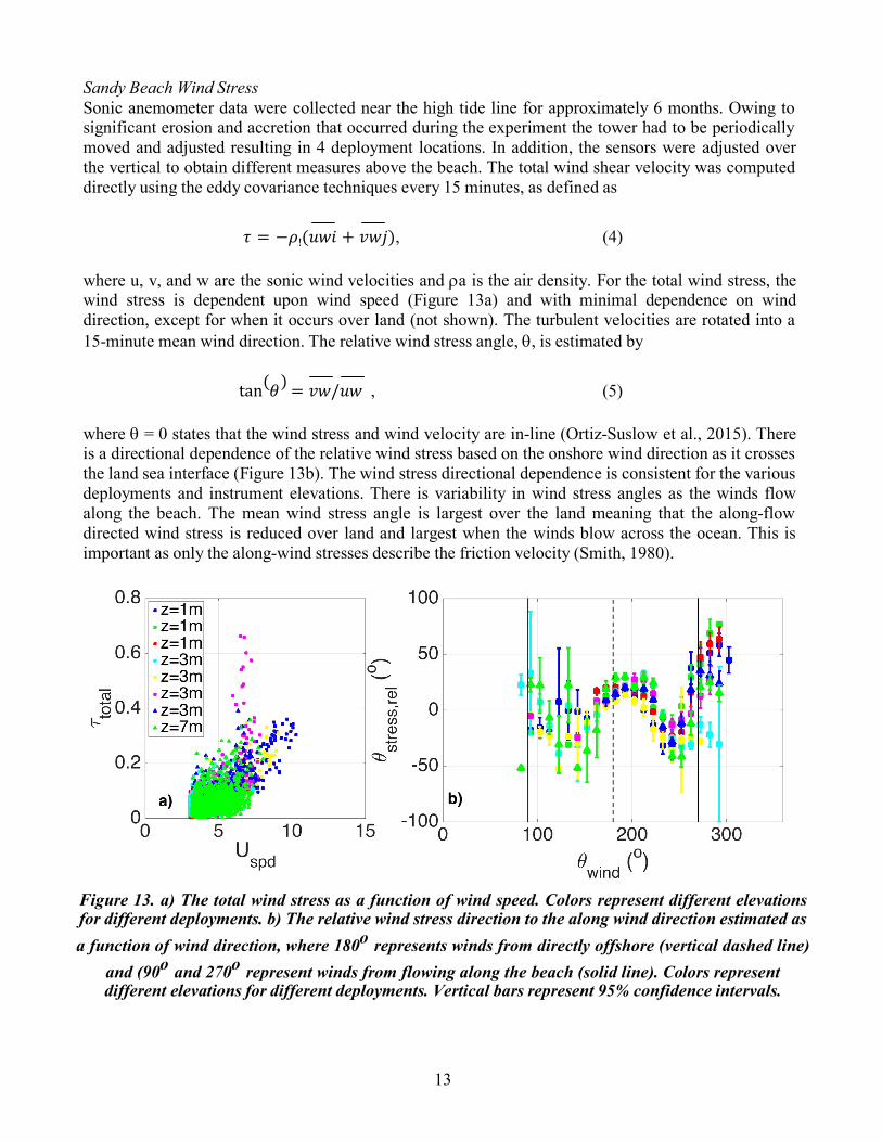
where u, v, and w are the sonic wind velocities and ρa is the air density. For the total wind stress, the wind stress is dependent upon wind speed (Figure 13a) and with minimal dependence on wind direction, except for when it occurs over land (not shown). The turbulent velocities are rotated into a 15-minute mean wind direction. The relative wind stress angle, θ, is estimated by

tan 𝜃 = 𝑣𝑤/𝑢𝑤 , (5)

where θ = 0 states that the wind stress and wind velocity are in-line (Ortiz-Suslow et al., 2015). There is a directional dependence of the relative wind stress based on the onshore wind direction as it crosses the land sea interface (Figure 13b). The wind stress directional dependence is consistent for the various deployments and instrument elevations. There is variability in wind stress angles as the winds flow along the beach. The mean wind stress angle is largest over the land meaning that the along-flow directed wind stress is reduced over land and largest when the winds blow across the ocean. This is important as only the along-wind stresses describe the friction velocity (Smith, 1980).

Figure 13. a) The total wind stress as a function of wind speed. Colors represent different elevations for different deployments. b) The relative wind stress direction to the along wind direction estimated as a function of wind direction, where 180o represents winds from directly offshore (vertical dashed line)

and (90o and 270o represent winds from flowing along the beach (solid line). Colors represent different elevations for different deployments. Vertical bars represent 95% confidence intervals.

14

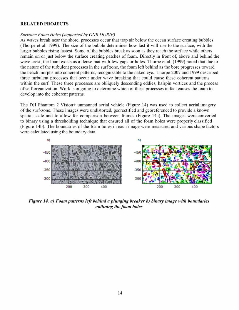
RELATED PROJECTS Surfzone Foam Holes (supported by ONR DURIP) As waves break near the shore, processes occur that trap air below the ocean surface creating bubbles (Thorpe et al. 1999). The size of the bubble determines how fast it will rise to the surface, with the larger bubbles rising fastest. Some of the bubbles break as soon as they reach the surface while others remain on or just below the surface creating patches of foam. Directly in front of, above and behind the wave crest, the foam exists as a dense mat with few gaps or holes. Thorpe et al. (1999) noted that due to the nature of the turbulent processes in the surf zone, the foam left behind as the bore progresses toward the beach morphs into coherent patterns, recognizable to the naked eye. Thorpe 2007 and 1999 described three turbulent processes that occur under wave breaking that could cause these coherent patterns within the surf. These three processes are obliquely descending eddies, hairpin vortices and the process of self-organization. Work is ongoing to determine which of these processes in fact causes the foam to develop into the coherent patterns. The DJI Phantom 2 Vision+ unmanned aerial vehicle (Figure 14) was used to collect aerial imagery of the surf-zone. These images were undistorted, georectified and georeferenced to provide a known spatial scale and to allow for comparison between frames (Figure 14a). The images were converted to binary using a thresholding technique that ensured all of the foam holes were properly classified (Figure 14b). The boundaries of the foam holes in each image were measured and various shape factors were calculated using the boundary data.

Figure 14. a) Foam patterns left behind a plunging breaker b) binary image with boundaries outlining the foam holes

15

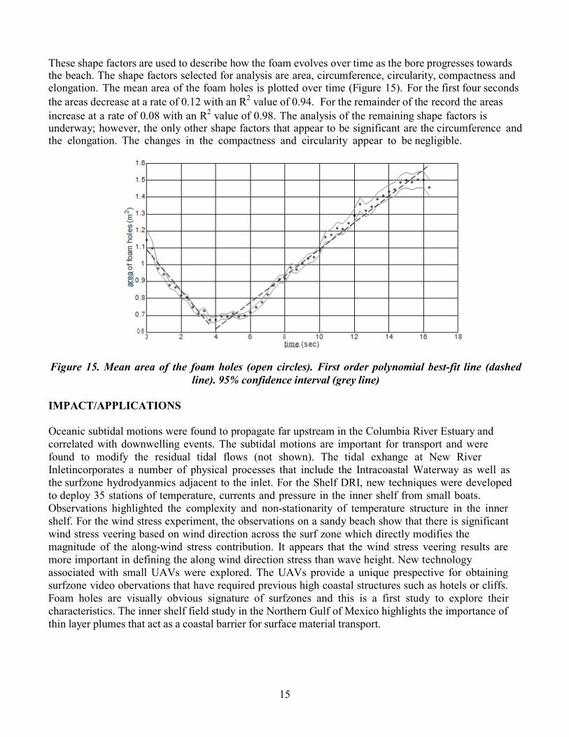
These shape factors are used to describe how the foam evolves over time as the bore progresses towards the beach. The shape factors selected for analysis are area, circumference, circularity, compactness and elongation. The mean area of the foam holes is plotted over time (Figure 15). For the first four seconds the areas decrease at a rate of 0.12 with an R2 value of 0.94. For the remainder of the record the areas increase at a rate of 0.08 with an R2 value of 0.98. The analysis of the remaining shape factors is underway; however, the only other shape factors that appear to be significant are the circumference and the elongation. The changes in the compactness and circularity appear to be negligible.

Figure 15. Mean area of the foam holes (open circles). First order polynomial best-fit line (dashed

line). 95% confidence interval (grey line) IMPACT/APPLICATIONS Oceanic subtidal motions were found to propagate far upstream in the Columbia River Estuary and correlated with downwelling events. The subtidal motions are important for transport and were found to modify the residual tidal flows (not shown). The tidal exhange at New River Inletincorporates a number of physical processes that include the Intracoastal Waterway as well as the surfzone hydrodyanmics adjacent to the inlet. For the Shelf DRI, new techniques were developed to deploy 35 stations of temperature, currents and pressure in the inner shelf from small boats. Observations highlighted the complexity and non-stationarity of temperature structure in the inner shelf. For the wind stress experiment, the observations on a sandy beach show that there is significant wind stress veering based on wind direction across the surf zone which directly modifies the magnitude of the along-wind stress contribution. It appears that the wind stress veering results are more important in defining the along wind direction stress than wave height. New technology associated with small UAVs were explored. The UAVs provide a unique prespective for obtaining surfzone video obervations that have required previous high coastal structures such as hotels or cliffs. Foam holes are visually obvious signature of surfzones and this is a first study to explore their characteristics. The inner shelf field study in the Northern Gulf of Mexico highlights the importance of thin layer plumes that act as a coastal barrier for surface material transport.

16

PUBLICATIONS (2014-2015) acknowledging ONR support Brown*, J.A., J. MacMahan, A. Reniers, E. Thornton, A.L. Shanks, S.G. Morgan, and E. Gallagher,

(2014) Mass Transport on a Steep Beach, in revision for Continental Shelf Research. Brown*, J.A., J. MacMahan, A. Reniers, E. Thornton (2015) Field observations of surfzone-inner shelf

exchange on a rip channeled beach, J. Physical Oceanography. MacMahan. J. (2015) Low frequency seiche in a Large Bay. J. of Physical Oceanography. MacMahan. J. (2015) Observations of oceanic-forced subtidal elevations in a convergent estuary. In

preparation. Roth, M.*, J. MacMahan, A. Reniers, K. Woodall, T. Ozgokmen, and B. Haus (2015) Observations of

surface material transport across the nearshore in the Northern Gulf of Mexico, submitted to J. Geophs. Res.

Rynne, P.F., A. Reniers, J. Van de Kreeke, J. MacMahan (2015) The Effect of Tidal Exchange on

Residence Time, resubmitted for Estuarine, Coasts, and Shelf Sciences. Swick* W., J. MacMahan, A. Reniers, Thornton (2014) Observations and modeling of transverse mixing

in a natural gravel-bed river, Journal of River Engineering, Vol. 2, Issue 9. Thornton, E.B., J. MacMahan , C. Gon, A. Reniers, S. Elgar (2015) Tidal wave reflection and distortion is

Elkhorn Slough, CA., in revision to J. of Geophys. Res. * Represents MacMahan’s Students Cited References Aubinet et al. (eds.) Eddy Covariance: A Practical Guide to Measurement and Data Analysis, Springer

Atmospheric Sciences, DOI 10.1007/978-94-007-2351-1_3 Buschman, F. A., A.J.F. Hoitink, M. van der Vegt, and P. Hoekstra, 2009. Subtidal water level

variation controlled by river flows and tides. Water Resources Res. 45, W10420, doi:10.1029/2009WR008167.

Flinchem, E. P. and D. A. Jay, 2000, An introduction to wavelet transform tidal analysis methods,

Estuarine Coastal Shelf Sci., 51, 177-200. Garvine, R. W., 1985, A simple model of estuarine subtidal fluctuations forced by local and remote

wind stress, J. Geophys. Res., 90, 11945-11948. Godin, G., 1999, The propagation of tides up rivers with special considerations on the upper Saint

Lawrence River, Estuarine Coastal Shelf Sci., 48, 207-324. Godin, G. and A. Martinez, 1994, Numerical experiments to investigate the effects of quadratic friction on

the propagation of tides in a channel, Cont. Shelf Res., 14, 723-748.

17

LeBlond, P. H., 1978, On tidal propagation in shallow rivers, J. Geophys. Res., 83 4717-4721. LeBlond,

P. H., 1979, Forced fortnightly tides in shallow waters, Atmos.- Ocean, 17, 253-264. Melville, W.K.,

1983, Wave modulation and breakdown, J. Fluid Mech. 128, 489-506.

Ortiz-Suslow, D. G., Haus, B. K., Williams, N. J., Laxague, N. J. M., Reniers, A., & Graber, H. C. (2015). The spatial-temporal variability of air-sea momentum fluxes observed at a tidal inlet. Journal of Geophysical Research-Oceans, 120(2), 660-676. doi:10.1002/2014jc010412

Shabani, B., Nielsen, P., & Baldock, T. (2014). Direct measurements of wind stress over the surf zone.

Journal of Geophysical Research-Oceans, 119(5), 2949-2973. doi:10.1002/2013jc009585 Smith, S. D. (1980), Wind stress and heat flux over the ocean in gale force winds, J. Phys. Oceanogr., 10,

709–726. Thorpe, S. A., W. A M. Nimmo Smith, A M. Thurnherr, and N. J. Walters, 1999: Patterns in foam.

Weather, 54, 327–334. Thorpe, S. A., 2007, An Introduction to Ocean Turbulence, Cambridge University Press, 235pp.