Discussion Papers

Turnout and ClosenessEvidence from 60 Years of Bavarian Mayoral Elections

Felix Arnold

1462

Deutsches Institut für Wirtschaftsforschung 2015

Opinions expressed in this paper are those of the author(s) and do not necessarily reflect views of the institute. IMPRESSUM © DIW Berlin, 2015 DIW Berlin German Institute for Economic Research Mohrenstr. 58 10117 Berlin Tel. +49 (30) 897 89-0 Fax +49 (30) 897 89-200 http://www.diw.de ISSN electronic edition 1619-4535 Papers can be downloaded free of charge from the DIW Berlin website: http://www.diw.de/discussionpapers Discussion Papers of DIW Berlin are indexed in RePEc and SSRN: http://ideas.repec.org/s/diw/diwwpp.html http://www.ssrn.com/link/DIW-Berlin-German-Inst-Econ-Res.html

Turnout and Closeness:

Evidence From 60 Years Of Bavarian Mayoral Elections

Felix Arnold∗

This Version: March 19, 2015

Abstract

One prediction of the calculus of voting is that electoral closenesspositively affects turnout via a higher probability of one vote beingdecisive. I test this theory with data on all mayoral elections in theGerman state of Bavaria between 1946 and 2009. Importantly, I useconstitutionally prescribed two-round elections to measure electoralcloseness and thereby improve on existing work that mostly uses ex-post measures that are prone to endogeneity. The results suggest thatelectoral closeness matters: A one standard deviation increase in close-ness increases turnout by 1.68 percentage points, which correspondsto 1

6 of a standard deviation in this variable. I also evaluate howother factors like electorate size or rain on election day affect turnoutdifferentially depending on the closeness of the race.

Keywords: Turnout, Closeness, Mayoral Elections,

Bavaria, Two-Round Ballot

JEL Classification: D72, H70

∗DIW Berlin and FU Berlin

1

1 Introduction

The well-known calculus of voting (Downs, 1957; Riker and Ordeshook, 1968)

postulates that the probability of influencing the electoral outcome is an

important determinant in the turnout decision. It predicts that electoral

participation should increase in the closeness of the race. Put differently,

when ”more is at stake,” people have an extra incentive to go to the polls.

However, it is not straightforward to measure electoral closeness in empirical

applications. How do people know whether the election is competitive or not?

Several approaches are used in the literature. Most existing studies rely on

ex-post realized closeness and assume rational expectations of the voters.

Apart from making a strong assumption, additional endogeneity concerns

arise. If vote shares appear on the right hand side and turnout on the left

hand side of the empirical model, the total number of votes cast appears on

both sides of the equation. Turnout and ex-post closeness may, therefore,

be spuriously correlated (Cox, 1988). As a consequence, other researchers

employ ex-ante historic closeness measures from previous elections to avoid

these issues. However, elections are not necessarily comparable across time,

especially if the set of candidates changes. The longer the electoral period,

the less useful is the information from a previous election. A third approach

therefore relies on pre-election opinion polls to gauge voters’ perception of

electoral closeness. However, these data are typically only available for large-

scale federal elections. It is unclear whether electoral closeness exists in this

context at all, because even a razor-thin victory in a large electorate may

translate into vote margins of tens of thousands of votes between winner and

runner up.

In this paper, a different approach is used. I employ two-round elections to

identify closeness effects. Mayoral elections in the German state of Bavaria

provide an ideal institutional setting: According to the local constitution in

Bavaria, if no mayoral candidate is able to get an absolute majority of the vote

in the first round, a second (runoff) election is held two weeks later with the

two leading candidates from the first round. Now, closeness of the first round

2

can be taken as a proxy for closeness of the second round. This measure,

which I call Revealed Closeness, avoids the drawbacks of other commonly used

measures in the literature. Revealed Closeness is predetermined and recent

at the same time, whereas other ex-ante (ex-post) measures only fulfill the

first (second) criterion. Another advantage of Bavarian mayoral elections lies

in the small size of the electorate. Municipalities in Bavaria can have as few

as 17 eligible voters. The largest city in the data still has fewer than 40,000

eligible voters. Thus, I can evaluate closeness effects in a setting where the

probability of being the decisive voter is non-negligible, which is rarely the

case in large-scale federal elections.

Using data on all mayoral elections in 2031 Bavarian municipalities between

1946 and 2009, I find that closeness does indeed matter for electoral partici-

pation: A one standard deviation increase in closeness increases turnout by

1.68 percentage points, which corresponds to 16

of a standard deviation in

this variable. Importantly, I show that Revealed Closeness, which makes use

of two-round elections, yields approximately the same results as the common

ex-post measures employed in the literature so far. Due to the panel structure

of the data, I can also evaluate a historical ex-ante measure of closeness. I

contribute to the literature by offering a first comparison of three differently

calculated indicators (ex-ante, ex-post, two-round) for electoral closeness. Im-

portantly, this comparison is conducted within one institutional framework.

Heterogeneous effects of other electoral stimuli, depending on closeness, are

also identified. For example, rain on election day reduces turnout on av-

erage, but not if the election is close. Furthermore, the negative effect of

constituency size on turnout is also mitigated by closeness. These findings

suggest that electoral closeness works as an important mediator. Other deter-

minants of turnout can thus be thought of as second rank – they matter only

if the race is not close. Implications for election campaigns are in contrast to

conventional wisdom: Usually, candidates running in several constituencies

concentrate their mobilization efforts on close races. My findings suggest,

however, that electoral stimuli work best in uncompetitive races and ques-

tion whether they have an effect in close races at all.

3

The remainder of this paper is organized as follows: Section 2 shortly presents

the theoretical background. Section 3 reviews the empirical literature on

turnout and electoral closeness. The institutional setting of Bavarian mayoral

elections and the data are described in Section 4. Section 5 holds descriptive

statistics and introduces the empirical strategy. Results are presented in

Section 6. Finally, Section 7 concludes.

2 Theoretical Considerations

Why should electoral closeness incite people to turn out to vote? The cal-

culus of voting developed by Downs (1957) and Riker and Ordeshook (1968)

contends that individuals compare the benefits and costs of voting in a ra-

tional choice manner.1 Let the net benefit of voting be described by the

following expression:

Y = πB +D −K (1)

Three factors determine Y , the net benefit of voting: πB is the expected

individual benefit of voting which depends on the outcome of the election.

It is comprised of π, the probability that a single vote will be decisive, and

B, the specific benefits that materialize if the preferred candidate wins and

takes office. D is a payoff that realizes independent of the electoral outcome.

It is often called the ”civic duty” component of the calculus of voting. K are

the (opportunity) costs of going to the polls.

An individual decides to cast a ballot if the benefits outweigh the costs of

voting, i.e. if Y > 0. Where does electoral closeness affect the turnout deci-

sion? The answer is that individuals will have a different perception of the

parameter π in close races. If one’s preferred candidate wins (or loses) for

sure, π is 0, and a single vote does not change that. As a consequence, πB

reduces to zero and does not influence the turnout decision any more. How-

ever, if the race is close, one vote can be decisive and π ∈ (0, 1]. Vice versa,

1For a summary of economic theories on voter turnout, see Dhillon and Peralta (2002).

4

abstaining could lead to a marginal loss of one’s preferred candidate.2 There-

fore, close races offer the possibility of discontinuously getting the additional

benefit B, which motivates people to turn out to vote. Put differently, the

potential pivotalness of a single vote increases in the closeness of the race.

Let closeness be denoted by c. Then we have

∂π

∂c> 0. (2)

As closeness positively impacts π, and π itself has a positive effect on the

turnout decision, closeness and turnout are positively related. Thus,

Y = π(c)B +D −K (3)

and

∂Y

∂c=∂Y

∂π

∂π

∂c= B

∂π

∂c> 0. (4)

Ceteris paribus, electoral closeness increases turnout by affecting the proba-

bility of a single vote being pivotal.

3 Empirical Literature

The interplay of closeness and turnout is a longstanding subject of debate

in economics and political science.3 The empirical focus is mostly on higher

2Some argue that even in close elections, the probability of being pivotal is essentiallyzero. As Schwartz (1987) put it, ”saying that closeness increases the probability of beingpivotal [...] is like saying that tall men are more likely than short men to bump theirheads on the moon.” I provide two answers to this objection. First, constituency size canbe extremely small in Bavarian mayoral elections. Some municipalities have no more than20 eligible voters. While closeness may play no role in state-wide ballots, it can make adifference in small Bavarian municipalities. Second, there is ample evidence that individ-uals have difficulties in handling small probabilities and hence overestimate the likelihoodof their vote being decisive (Fehr-Duda and Epper, 2012; Kahneman and Tversky, 1979).Closeness thus increases turnout depending on the perceived probability of being pivotal,not the actual probability of being pivotal.

3A specific branch of the literature deals with the partisan effects of voter turnout.Hansford and Gomez (2010) use election day rain as an instrument for turnout and findthat higher turnout helps the Democrats in US presidential elections. In a similar fashion,Gomez, Hansford, and Krause (2007) estimate that one inch of rain reduces turnout in a

5

level elections. Endersby, Galatas, and Rackaway (2002) find that closeness

positively impacts turnout in the 1993 / 1997 Canadian federal elections,

controlling for campaign expenditures. The same effect is established for the

1982 US House election by Cox and Munger (1989). Shachar and Nalebuff

(1999) develop a structural model to evaluate feedback effects between close-

ness, turnout and mobilization efforts of political leaders. They estimate

that a one percent increase in electoral closeness increases turnout by 0.34

percent. In Germany, a small positive closeness effect is found for the federal

elections from 1983 to 1994 (Kirchgassner and Zu Himmern, 1997). However,

the robustness of the effect seems to be confined to West Germany. Grof-

man, Collet, and Griffin (1998) argue that in US Senate and House elections

turnout is not maximized at maximal closeness (i.e. the 50-50 split of the

vote), but at a Republican share greater than 50 percent. According to the

authors, this happens because Republican partisans are generally more likely

to vote. For Swiss referendums between 1981 and 1999, mobilization effort

is a better predictor of turnout than expected closeness (Kirchgassner and

Schulz, 2005). All these studies use an ex-post measure of electoral close-

ness. For a review and meta-analysis of all empirical studies explaining voter

turnout, see Geys (2006).

A more direct test of the people’s reaction to the parameter π in the calculus

of voting is provided by Tukiainen and Lyytikainen (2013). Using exogenous

variation in pivotal probabilities that occur at population thresholds where

council size changes discontinuously, the authors show that turnout is higher

just above the thresholds where the probability of being pivotal increases

and conclude that ”voters are rational.” Andersen, Fiva, and Natvik (2014)

find that in Norway, people are more likely to vote when more is at stake in

the election. Due to topography-determined exogenous hydropower income

of some municipalities, they can evaluate how people respond to changes in

the size of the parameter B in the calculus of voting. According to their

county by roughly 0.8 percent. Related, one inch above normal rain gives the Republicancandidate an extra 2.5 percent of the vote. For Germany, Arnold and Freier (2015) findthat social democrats profit from higher turnout levels. Conservatives, on the contrary,seem to suffer under higher electoral participation.

6

estimates, a change in hydropower income from minimum to maximum in-

creases turnout by six percentage points. Fraga and Hersh (2010) provide a

first estimate of the interaction between closeness and inclement weather on

election day using county data for US Presidential elections. In the calculus

of voting, rain works as an exogenously imposed cost on the act of voting,

that is, it is equivalent to an increase in the parameter K. They find that

rain negatively impacts turnout on average, but this effect is mitigated in

close elections. Closeness is calculated both with an ex-ante as well as an

ex-post measure.

There is a small and recent literature that also uses two-round elections

to identify closeness effects (De Paola and Scoppa, 2014; Fauvelle-Aymar

and Francois, 2006; Garmann, 2014; Indridason, 2008; Simonovits, 2012).4 I

contribute to this literature and extend it by offering two innovations: First,

the long panel data allow to credibly evaluate measures of lagged closeness

and provide sufficient variation to include electorate fixed effects into the

model. Second, the use of precipitation data is still quite rare in turnout

applications. I offer a first estimate of the interaction effect between electoral

closeness and inclement weather on election day for an election outside the

United States.5

4Two-round elections are also used to measure so-called bandwagon effects (Ade andFreier, 2013; Kiss and Simonovits, 2014) or to study the formation of electoral pacts (Blaisand Indridason, 2007).

5The data on Bavarian mayoral elections employed in this paper have been used before-hand. Freier (2011) estimates party incumbency effects in the order of 38-40 percentagepoints in the probability of winning the next mayoral election. In a related paper, Freierand Thomasius (2012) find that more qualified candidates receive higher vote shares. Fur-thermore, social-democratic mayors seem to reduce local taxes, while conservative mayorsincrease taxes (Freier and Odendahl, 2012). Schild (2013) asks whether female mayors al-locate municipal budgets to different categories than their male counterparts and finds nosignificant differences. All these studies rely on Regression Discontinuity Designs (RDD)to estimate causal effects. On the validity of RDD in electoral contexts, see Eggers, Fowler,Hainmueller, Hall, and Snyder (2015), who also use the data on Bavarian mayoral elections.

7

4 Institutional Setting and Data

Bavaria is Germany’s largest state by area and has about 12.6 million inhab-

itants (as of June 2014). The governing structure is organized into several

administrative layers: In total, there are 2056 municipalities (including 25

county-free cities), 96 counties, and 7 administrative regions. Hence, mu-

nicipalities constitute the smallest organizational unit of government. They

are governed by a mayor (executive branch) and a town council (legislative

branch). The mayor is also a full member of the town council and serves as

its president. Once elected, the mayor is the highest representative of the

municipality and executes decisions taken by the council. Larger munici-

palities have full-time mayors that are employed as public servants. Smaller

municipalities (with less than 5000 inhabitants) often have honorary mayors.6

Since the end of World War II, each Bavarian municipality directly elects its

mayor. Each citizen above the age of 18 is allowed to vote. Running as a

candidate is possible from age 21 onwards. To win the election in the first

round, an absolute majority of votes is necessary. If no candidate is able

to gather more than 50 percent of the votes, then a runoff election is held

two weeks after the first election. The two leading candidates from the first

round advance to the second round. Whoever gathers a majority of votes

in the runoff election is the newly elected mayor. A mayoral term lasts six

years.7 Around 85 percent of the elections are held in March or the beginning

of April. The remaining 15 percent are distributed relatively evenly over the

year.8

I have data on all Bavarian mayoral elections between 1946 and 2009. With

27015 observations in total and 2031 municipalities,9 this makes about 13

6More detailed information on tasks and status of the mayor can be found inthe Bavarian municipal code (Gemeindeordnung, GO), articles 34-39, accessible viawww.gesetze-bayern.de.

7The detailed elecoral rules are laid down in the Bavarian electoral law for municipalitiesand counties (Gemeinde- und Landkreiswahlgesetz, GLKrWG), articles 39-52, accessiblevia www.gesetze-bayern.de.

8The ”official” election date is in March. However, if an incumbent resigns or retiresbefore the end of the electoral period, early elections can be called.

9Mayoral election results for the 25 county-free cities are missing.

8

elections per municipality on average. The data are from the state statis-

tical office and include a variety of information. For example, I know all

candidates’ names, gender, profession and party affiliation. Furthermore, in-

formation on the exact election day, the number of eligible voters, the number

of voters who turned out and individual candidate vote shares are available.

I also know the status of the mayor (full-time vs. honorary) and whether a

runoff election was held or not.

I combine these mayoral election data with precipitation data from 559

weather stations in Bavaria. These daily time series data are recorded and

published by the German Weather Service (Deutscher Wetterdienst, DWD).

As I know geographic locations of municipalities and weather stations as well

as the exact election dates, I can tell exactly how much it rained on election

day in a given municipality (which is assigned to the nearest weather sta-

tion). Figure 1 in the appendix shows a map of Bavaria with all weather

stations marked by blue dots.

5 Descriptives and Empirical Strategy

Before looking at the data, one note of caution is in order. To this day,

the literature has not yet agreed on one commonly used measure of electoral

closeness.10 Most authors use variations of vote margins between winner and

runner-up.11 The disadvantage of this measure is its interpretability. When

vote margins are introduced as closeness proxy in a regression framework,

signs are reversed. Higher closeness is equivalent to smaller vote margins

and vice versa. To ease readability, I use a variation of the vote margin as

10See Endersby, Galatas, and Rackaway (2002) for development of a competitivenessindex and a comparison of different closeness indicators in Canadian federal elections.See Kayser and Lindstaedt (2015) for a cross-nationally applicable measure of electoralcompetitiveness.

11In a methodological note, Cox (1988) warns that vote margins – when introducedas explanatory variables in a regression framework – are spuriously correlated with thedependent variable turnout. He suggests to use raw vote margins instead. Note that hiscriticism does not apply to my approach, because I use vote margins from the first roundand turnout from the second round. My closeness measure is thus predetermined and notendogenous to turnout.

9

an indicator for closeness:

Closeness = 1− (vs1 − vs2) (5)

where vsi is the vote share of the candidate finishing ith place. With this

definition, the closeness variable is bounded between 0 and 1 and has a

positive sign. A value of 1 indicates maximum closeness: There is a tie for

first and second place. A value of 0, on the contrary, signals that the election

was not close at all. Either the first place candidate was able to garner all

the votes, or there was simply no contender.

Descriptive statistics of all variables used in the analysis can be found in

Tables 2, 3 and 4 in the appendix. I distinguish between three different

types of elections: Table 2 contains information on ”uncontested elections,”

i.e. elections with low competition where one candidate is able to gather

more than 50 percent of the vote in the first round. Most elections are

uncontested. Table 3 holds the same statistics for ”contested elections.”

These are first round elections where no single candidate is able to receive

an absolute majority of votes. Finally, Table 4 shows descriptive statistics

for runoff elections. These elections automatically follow contested elections

and only the two leading candidates from the first round are allowed to run

in the second round.

Several differences emerge between the different samples. Turnout is lower

in runoff elections, indicating voter fatigue and dissatisfaction when one’s

preferred candidate does not reach the second round. Nevertheless, the over-

all turnout levels – at about 80 percent – are quite high compared to state

or federal elections. Closeness is highest in contested elections and lowest

in uncontested elections, as one would expect. The distributions of turnout

and closeness in the three different samples are visualized in Figure 2 in the

appendix. Elections are more likely to be contested when electorate size is

larger and when more candidates decide to run. Surprisingly, elections for

honorary mayor positions are contested more often than the ones for full-time

mayor positions. The maximum number of eligible voters is 38461 and hence

10

quite small. This reflects the fact that mayoral elections in the 25 county-

free cities, which constitute the largest cities, are not recorded in the dataset.

Females are more likely to run in contested elections, although their overall

share of the candidate pool is never larger than 15 percent. The well-known

lack of women in politics (Ferreira and Gyourko, 2014; Lawless and Pearson,

2008) is strikingly visible in Bavarian mayoral elections.12

Given that weather is essentially random, it is not surprising that the rain

variables do not show substantial differences in the various subsamples. In

Table 2, rain on election day amounts to 1.9 millimeters on average. However,

this includes all election days with no rain at all, which constitute almost 60

percent of the sample. Conditional on some rain at all, average rainfall on

election day rises to 1.8680.585

= 3.193 millimeters.13 The quality and accuracy of

the weather data are captured by the distance to the nearest weather station.

As the grid of weather stations is quite dense in Bavaria (see Figure 1), there

is no municipality located further away than 14 kilometers from the next

station. Average distance is below 5 kilometers.14

Due to the panel structure of the data and the special institutional setting

where some (but not all) elections have a second (runoff) round, I can eval-

uate three different measures of closeness and compare them:

Lagged Closeness takes closeness from the preceding regular election as the

crucial measure. As this is lagged by six years or one electoral period, it

is known to the voters on election day (it is ex-ante). However, it contains

information on an election with possibly completely different circumstances

/ political constellations than the current election.

12Related, Freier and Thomasius (2012) find that female candidates in Bavaria suffer anelectoral disadvantage of roughly five percent in vote share.

13As most elections take place in (relatively) rainy March, the variation in rain acrosstime and space is quite high.

14Note that the number of observations is somewhat smaller for the rain variables. Thisis due to the fact that some weather stations were inaugurated only later in the sampleperiod. In principle, I could match uncovered early elections to weather stations furtheraway and retain all observations. However, this comes at the cost of bringing more noiseinto the weather variables. Given that precipitation (and especially rain showers) can bequite local, I decided against the matching over longer distances.

11

Actual Closeness takes on the value of the ex-post realized closeness of the

current election. As this is generally unknown on election day, one has to

assume rational expectations of the voters if this measure is supposed to

influence their decision to turn out or not.

Revealed Closeness makes use of two-round elections. Closeness of the first

round is taken as a signal for competitiveness of the second round two weeks

later. This measure is superior to the two previous ones: It is recent (contrary

to Lagged Closeness) and predetermined (contrary to Actual Closeness) at

the same time.

The basic empirical model looks as follows:

Tit = α + βCit +X ′itω + θi + εit. (6)

The dependent variable Tit is turnout in municipality i at date t. I define

turnout as the number of voters that go to the polls divided by the number

of eligible voters. Cit is the closeness of the election, according to the three

different concepts introduced above and calculated as in Equation 5. For

actual and lagged closeness, I use the sample of uncontested elections. To

evaluate the effect of revealed closeness on turnout, I use the sample of runoff

elections and add closeness from contested elections two weeks prior. The

vector of control variables X includes a third order time trend, a third order

polynomial in the number of eligible voters, a dummy for concurrent elec-

tions, dummies for female candidates and honorary mayor positions as well

as the lagged dependent variable (to account for ”usual” levels of electoral

participation). I also add dummies for the number of candidates. Fixed

effects for each municipality i are included in θi, where i = 1, 2, ..., 2031.

Standard errors are robust to heteroscedasticity.

12

6 Results

6.1 Main Results

Table 1 shows regressions of turnout on the three different measures of elec-

toral closeness.

Column (1) holds the results for Lagged Closeness using the sample of un-

contested elections. One can see that lagged closeness exerts a small negative

impact on turnout, which is unexpected and stands in contrast to the theo-

retical considerations introduced above. I argue, however, that this measure

is confounded with incumbency effects that materialize over time. Assume

that the last election was very close (i.e. a high value of Lagged Closeness).

It is quite likely that this last election was a hard-fought race for an open

seat. Then one of the candidates won and took office. In the current election,

he is the incumbent and profits from substantial incumbency advantages, as

shown in Freier (2011). Therefore, the race is not close and people abstain

from voting. Thus, a high value of Lagged Closeness is associated with low

levels of turnout today due to incumbency effects that materialize between

the two elections. In a setting like Bavaria, where incumbency effects are im-

portant in magnitude,15 measures like Lagged Closeness are of limited value.

Column (2) presents results for Actual Closeness. Here, the coefficient is

in line with theoretical expectations. If closeness switches from 0 to 1 (i.e.

from minimum to maximum), turnout increases by 5.3 percentage points.

Another way to look at the coefficient is the following: A one standard

deviation increase in Actual Closeness (0.325) leads to a turnout rate that is

0.053 · 0.325 ≈ 1.72 percentage points higher, which roughly corresponds to

a 15

standard deviation increase in this variable.

Finally, column (3) shows results for the measure of Revealed Closeness,

which makes use of two-round elections. Also here, the coefficient of interest

is positive and significant, as anticipated. It is also four to five times as

15Freier (2011) estimates that incumbency status increases the probability of winningthe next election by 38-40 percentage points.

13

Table 1: Main Results

(1) (2) (3)Turnout Turnout Turnout

Sample Uncontested Elections Runoff Elections

Lagged Closeness -0.012***(0.001)

Actual Closeness 0.053***(0.002)

Revealed Closeness 0.234***(0.020)

Turnout in Preceding Election 0.213*** 0.188*** 0.865***(0.011) (0.010) (0.042)

Concurrent Election 0.067*** 0.066*** 0.071***(0.006) (0.007) (0.024)

Female Candidate(s) -0.000 -0.000 0.001(0.002) (0.002) (0.005)

Honorary Mayor 0.002 0.003 0.004(0.002) (0.002) (0.005)

Two Candidates 0.057*** 0.025***(0.001) (0.002)

Three Candidates 0.067*** 0.036*** 0.004(0.002) (0.002) (0.009)

Four Candidates 0.071*** 0.040*** -0.001(0.004) (0.004) (0.010)

Five Candidates 0.065*** 0.034*** -0.014(0.008) (0.008) (0.010)

Six Candidates 0.083*** 0.052*** 0.001(0.011) (0.010) (0.012)

Seven Candidates 0.103*** 0.073*** 0.007(0.011) (0.008) (0.012)

Constant 0.690*** 0.701*** -0.147***(0.011) (0.010) (0.045)

Municipal Fixed Effects yes yes yesThird Order Electorate Size Polynomial yes yes yesThird Order Time Trend yes yes yes

N 20582 20582 1859R2 0.64 0.65 0.83

Notes: Standard errors robust to heteroscedasticity. Significance Levels: * p < 0.10, ** p < 0.05,*** p < 0.01. The data cover all mayoral elections in 2031 Bavarian municipalities from 1946-2009.

large as in column (2). However, one has to keep in mind that Revealed

Closeness only varies between 0.5 and 1, because it is calculated from the

14

contested election two weeks prior where no single candidate was able to

garner more than 50 percent of the vote. Putting the size of the coefficient

into perspective, a one standard deviation increase in Revealed Closeness

(0.072) leads to a turnout rate that is 0.234 · 0.072 ≈ 1.68 percentage points

higher. This corresponds to roughly 16

of a standard deviation in this variable.

Figure 3 in the appendix shows the slope coefficients of lagged, actual and

revealed closeness in the turnout equation and thereby visualizes the findings

from Table 1.

The coefficients of the control variables also merit a short discussion. Turnout

in the preceding election has a large and significant impact on current turnout

in all three specifications. Given that the preceding election happened six

years ago in columns (1) and (2), it is not surprising that the coefficient is

much larger in column (3), where the preceding election was much more re-

cent, namely two weeks ago. If another election (federal, state or European

level) is held on the same day as the mayoral election, turnout is approxi-

mately seven percentage points higher, as captured by the dummy variable

Concurrent Election. Statistically, it does not seem to make a difference for

electoral participation whether female candidates run for office or not. The

same holds true for the status of the mayor: Races for honorary and full-

time positions show turnout rates that are not statistically different from

each other.16

The dummies for the number of candidates show the expected signs. More

candidates lead to higher turnout rates, ceteris paribus. As discussed in the

theory section, this effect can be due to higher aggregate mobilization efforts

or to a higher likelihood of finding a candidate on the ballot sheet that is

close to one’s own political views. In runoff elections (column (3)), only two

candidates remain. The number of candidates in the first round does not

seem to have an impact on turnout levels in the second round.

16As mayor status depends on municipal size and I already control for the number ofeligible voters, this finding is not too surprising.

15

All models include fixed effects for each municipality, a third order polyno-

mial to control for electorate size and a third order time trend to capture

structural developments in turnout rates over time. The coefficients are not

reported in detail, but some remarks are in order.

Turnout and electorate size are negatively related.17 In line with theory,

turnout is lower in larger municipalities where the probability of being pivotal

is close to zero. Figure 4 in the appendix graphically shows the negative slope.

Furthermore, turnout rates are trending downwards over time.18 This trend

– visualized in Figure 5 in the appendix – is consistent with evidence from

other developed democracies like the US (see for example Gentzkow (2006)).

Interestingly, electoral closeness seems to have increased over time, at least

in uncontested elections. This finding is lacking a theoretical explanation

so far. The R2 of the regressions is quite high and lies between 0.64-0.83,

highlighting the large explanatory power of the right hand side variables.19

6.2 Heterogeneous Effects

It is worthwhile to take a closer look at other variables that affect the costs

and benefits of voting. I have already shown that electorate size negatively

affects turnout by reducing the probability of one vote being decisive, i.e. by

reducing π in the calculus of voting. Rain on election day is a factor that

increases the costs of voting (K ↑) and should therefore negatively influence

turnout. In what follows, I test if voters react differently to larger electorate

sizes or rain on election day when the race is closer.

I therefore estimate the following interaction specification

Tit = α + βCit + γVit + δRit + ρCitVit + ψCitRit +X ′itω + θi + εit (7)

17To be more specific, the coefficient of the linear term of Voters is negative, the squareis positive and the cube is again negative.

18Also here, the linear term of the Year variable is negative, the square is positive, andthe cube is again negative.

19Dropping the lagged dependent variable decreases the R2 by 10-15 percent, dependingon the specification.

16

where Vit is the number of eligible voters, Rit is rain in millimeters and ρ and ψ

are coefficients of interaction effects of these two variables with the closeness

variable. All other variables and parameters are described in Equation 6 and

all controls from the baseline regression are included.

Table 5 in the appendix holds the results. In columns (1) - (3), I interact the

three closeness measures with the number of eligible voters in the municipal-

ity. Columns (4) - (6) show analogous results when closeness is interacted

with the amount of rain on election day (measured in millimeters). The

interacted variables are always included linearly, too.

As evident from columns (2) and (3) in Table 5, constituency size (as mea-

sured by the variable Voters) has a negative impact on turnout, but this

effect is mitigated in close elections, as shown by the positive sign of the

interaction term. This holds for the measures of actual and revealed close-

ness, whereas the coefficient of Lagged Closeness again has the opposite sign.

The regressions with the rain variables in columns (4) - (6) also reveal some

interesting insights. First, rain on election day reduces turnout, albeit at a

small scale.20 The coefficient in column (5) implies that 10 millimeters of

rain reduce turnout by one percentage point.2122 However, given the max-

imum amount of precipitation recorded on election day (84.3 millimeters),

it becomes clear that weather can be a non-negligible factor. Importantly,

I control for location-specific general precipitation patterns by including the

average amount of rain that usually falls on election day in a municipality

into the model. Rain levels above (or below) that level cannot be anticipated

by the voters and hence act as a random cost (benefit) on the act of voting.

20Election days with no rain at all also have lower turnout levels, as can be seen bythe negative coefficient of the No Rain dummy. This puzzling result could be due to anomitted variable: If days with no rain at all are especially sunny and warm, opportunitycosts of voting might again go up because people want to make use of the good weather.Although data on temperatures and hours of sunshine are available, the grid of weatherstations recording these data is much looser than the grid recording the precipitation data.In order to prevent the inclusion of noisy data, I focus on the rain variables.

21This effect is of similar magnitude as the effects reported by Arnold and Freier (2015)for municipal and state elections in the German state of North-Rhine Westphalia.

22I also experimented with a quadratic specification of the rain variable, but the squareterm never reached conventional levels of statistical significance.

17

Again, the negative effect of rain is mitigated when closeness is higher, as

indicated by the positive signs of the interaction terms in columns (5) and

(6).

These results suggest that the competitive context of an election plays an

important role. On rainy days, people vote less on average, but not if the

race is close. Larger electorates have lower turnout rates in uncompetitive

environments, but the number of voters does not matter as much when some

candidates have equal chances of winning. My findings show that electoral

closeness is an important mediator when it comes to the functioning of elec-

toral stimuli. Figure 6 in the appendix shows the different slope coefficients

of electorate size and rain in uncompetitive vs. competitive environments

and thereby visualizes the findings from Table 5.

6.3 Robustness

Until now, all models have been estimated with municipal-level fixed effects.

Hence, the closeness effects were largely identified from the within varia-

tion in the data. The results remain entirely robust without the municipal

fixed effects. Including county or administrative region fixed effects does not

change the qualitative or quantitative results either. Furthermore, I clustered

the standard errors at these higher levels. The statistical significance of the

findings was never affected (all results available upon request).

6.4 Attenuation Bias and IV Strategy

Using Revealed Closeness addresses the endogeneity issues that would oth-

erwise arise when relying on Actual Closeness only. Garmann (2014), how-

ever, argues that also first-round competition measures voters’ expectation of

electoral closeness only with an error, thereby creating an errors-in-variables

problem. To get rid of potential remaining attenuation bias, he suggests to

use an IV strategy where closeness of the second round is instrumented with

closeness from the first round. As a further robustness check, I provide such

estimates in Table 6 in the appendix. Revealed Closeness is a strong predictor

18

of Actual Closeness. An F-Statistic of more than 100 indicates that the in-

strument is highly relevant. The effect of instrumented closeness on turnout

is consistent with the main findings in Table 1, albeit being somewhat larger.

7 Discussion

In this paper, I examine whether turnout is higher in close elections. Using

an ex-ante, an ex-post and a two-round measure of electoral closeness, I find

that closeness does indeed matter: If the election is very competitive, people

go to the polls at a higher rate. This is a surprising result, given the actual

probability of influencing the outcome with one’s own vote: In all 27015

Bavarian mayoral elections between 1946 and 2009, there are only 33 cases

where one vote would have changed the outcome. This corresponds to a

probability of being pivotal in the order of 3327015

= 0.0012 ≈ 0.12 percent. A

tentative explanation for the positive closeness effect is that voters’ turnout

decision is based on the perceived probability of being pivotal, not the actual

probability. Likewise, one could interpret voting in relatively close elections

as a type of insurance against the worst case: Even though the probability of

being pivotal is close to zero, voters want to avoid the trouble of not having

voted and realizing that their vote would have changed the outcome after all.

Furthermore, I provide evidence that other electoral stimuli, like electorate

size and rain showers on election day, affect turnout differently depending

on the competitive context of the election. In this sense, closeness works

as a mediator, making other costs of voting less important in the turnout

decision. Implications for campaigners and candidates are straightforward:

If rain impacts turnout only conditional on (non-)closeness, it is quite likely

that other classic mobilization tactics like get-out-to-vote campaigns or ad-

vertisements work better or worse depending on the closeness of the race. If

the competitive context is ”first order,” election campaigns should take this

into account.

My results also have implications for the literature on electoral closeness.

First, I show that the two measures ex-post Actual Closeness and ex-ante

19

Revealed Closeness display comparable effects on turnout. Therefore, the

many studies relying only on ex-post Actual Closeness – due to data limita-

tions and lack of two-round elections – do not make a mistake. However, the

results also show that historical measures of closeness dating back to a previ-

ous election (Lagged Closeness) are potentially confounded with incumbency

effects and therefore biased. Of course, this interpretation of the findings is

based on the assumption that Revealed Closeness identifies the true effect of

electoral closeness on turnout.

20

Appendix

Table 2: Summary statistics: Uncontested Elections

Variable Mean Std. Dev. Min. Max. N

Turnout 0.813 0.091 0.222 1 22813Closeness 0.394 0.325 0 1 22813Voters 2086.371 2639.56 17 38461 22813Number of Candidates 1.632 0.756 1 7 22813Concurrent Election 0.009 0.095 0 1 22813Female Candidate(s) 0.037 0.189 0 1 22813Honorary Mayor 0.262 0.44 0 1 21079

No Rain 0.585 0.493 0 1 18791Rain in mm 1.868 4.128 0 84.3 18791Day Station Average Rain in mm 2.254 1.021 0.1 11.743 18791Distance to Nearest Weather Station in km 4.835 2.324 0.025 13.899 22813Altitude in m 464.891 170.589 107 1832 18791

Table 3: Summary statistics: Contested Elections

Variable Mean Std. Dev. Min. Max. N

Turnout 0.808 0.089 0.423 1 2284Closeness 0.904 0.072 0.515 1 2284Voters 3518.558 4023.755 20 34694 2284Number of Candidates 3.105 0.858 1 7 2284Concurrent Election 0.014 0.118 0 1 2284Female Candidate(s) 0.145 0.353 0 1 2284Honorary Mayor 0.483 0.5 0 1 2284

No Rain 0.636 0.481 0 1 1870Rain in mm 1.585 3.778 0 32.8 1870Day Station Average Rain in mm 2.171 0.895 0 8.18 1870Distance to Nearest Weather Station in km 4.761 2.432 0.025 13.899 2284Altitude in m 455.498 161.768 110 1832 1870

21

Table 4: Summary statistics: Runoff Elections

Variable Mean Std. Dev. Min. Max. N

Turnout 0.758 0.106 0.351 0.974 1892Closeness 0.867 0.106 0.198 1 1892Voters 3988.797 4228.991 144 34658 1892Number of Candidates 1.999 0.023 1 2 1892Concurrent Election 0.005 0.069 0 1 1892Female Candidate(s) 0.078 0.268 0 1 1892Honorary Mayor 0.483 0.5 0 1 1873

No Rain 0.588 0.492 0 1 1657Rain in mm 2.386 4.716 0 39.9 1657Day Station Average Rain in mm 2.239 0.943 0.05 8.898 1657Distance to Nearest Weather Station in km 4.768 2.469 0.025 13.899 1892Altitude in m 455.879 163.552 110 1832 1657

Figure 1: Grid of Weather Stations in Bavaria

Notes: This map presents the spatial distribution of all 559 weather stations in Bavaria. The black linesdepict the borders of all 2056 municipalities. Each blue dot stands for a weather station.

22

Figure 2: Distributions of Turnout and Closeness

01

23

45

Den

sity

0 .2 .4 .6 .8 1Turnout

Uncontested Elections

02

46

Den

sity

0 .2 .4 .6 .8 1Turnout

Contested Elections

01

23

4D

ensi

ty

0 .2 .4 .6 .8 1Turnout

Runoff Elections0

12

34

Den

sity

0 .2 .4 .6 .8 1Closeness

Uncontested Elections

02

46

8D

ensi

ty

0 .2 .4 .6 .8 1Closeness

Contested Elections

01

23

45

Den

sity

0 .2 .4 .6 .8 1Closeness

Runoff Elections

Figure 3: Turnout and Closeness

.65

.7.7

5.8

.85

.9T

urno

ut

0 .2 .4 .6 .8 1Lagged Closeness

Observed Data

Local Polynomial Smooth

Fitted values

.65

.7.7

5.8

.85

.9T

urno

ut

0 .2 .4 .6 .8 1Actual Closeness

Observed Data

Local Polynomial Smooth

Fitted values

.65

.7.7

5.8

.85

.9T

urno

ut

0 .2 .4 .6 .8 1Revealed Closeness

Observed Data

Local Polynomial Smooth

Fitted values

23

Figure 4: Turnout and Electorate Size

.2.4

.6.8

1T

urno

ut

0 5000 10000 15000Number of Eligible Voters

Observed Data Fitted Values

Figure 5: Turnout and Closeness Over Time

0.2

.4.6

.81

Clo

sene

ss, T

urno

ut

1940 1960 1980 2000 2020Year

Turnout Fitted values

Actual Closeness Fitted values

Uncontested Elections

0.2

.4.6

.81

Clo

sene

ss, T

urno

ut

1940 1960 1980 2000 2020Year

Turnout Fitted values

Revealed Closeness Fitted values

Runoff Elections

Notes: Bold circles and triangles represent years in which a major election took place (roughly 2000municipalities), while the smaller circles and triangles represent years which do not belong to the usualelection cycles (generally less than 100 observations). The fit lines are generated using equal weighting ofall years.

24

Table 5: Heterogeneous Effects: Electorate Size and Weather

(1) (2) (3) (4) (5) (6)Turnout Turnout Turnout Turnout Turnout Turnout

Sample Uncontested Elections Runoff Elections Uncontested Elections Runoff Elections

Lagged Closeness -0.007*** -0.011***(0.002) (0.002)

Actual Closeness 0.037*** 0.051***(0.003) (0.003)

Revealed Closeness 0.214*** 0.222***(0.020) (0.021)

Turnout in Preceding Election 0.217*** 0.190*** 0.856*** 0.195*** 0.175*** 0.842***(0.011) (0.010) (0.041) (0.013) (0.011) (0.045)

Voters -0.157*** -0.199*** -0.111** -0.172*** -0.175*** -0.022(0.016) (0.016) (0.045) (0.017) (0.017) (0.047)

No Rain -0.004*** -0.003*** 0.002(0.001) (0.001) (0.004)

Rain in mm -0.000* -0.001*** -0.011***(0.000) (0.000) (0.004)

Day Station Average Rain in mm -0.003*** -0.003*** 0.003(0.000) (0.001) (0.001)

Constant 0.456*** 0.500*** -0.197*** 0.485*** 0.519*** -0.204***(0.010) (0.010) (0.027) (0.012) (0.011) (0.029)

Interaction Effects

Lagged Closeness * Voters -0.026***(0.009)

Actual Closeness * Voters 0.068***(0.010)

Revealed Closeness * Voters 0.073***(0.017)

Lagged Closeness * Rain 0.000(0.000)

Actual Closeness * Rain 0.001***(0.000)

Revealed Closeness * Rain 0.013***(0.004)

All Controls from Baseline Regression yes yes yes yes yes yes

N 20582 20582 1859 17386 17386 1632R2 0.64 0.65 0.83 0.64 0.65 0.83

Notes : Standard errors robust to heteroscedasticity. Significance Levels: * p < 0.10, ** p < 0.05, *** p < 0.01. The data coverall mayoral elections in 2031 Bavarian municipalities from 1946-2009. The coefficient of Voters has been multiplied by 104 toease readability.

25

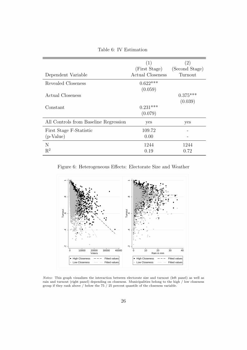
Table 6: IV Estimation

(1) (2)(First Stage) (Second Stage)

Dependent Variable Actual Closeness Turnout

Revealed Closeness 0.622***(0.059)

Actual Closeness 0.375***(0.039)

Constant 0.231***(0.079)

All Controls from Baseline Regression yes yes

First Stage F-Statistic 109.72 -(p-Value) 0.00 -

N 1244 1244R2 0.19 0.72

Figure 6: Heterogeneous Effects: Electorate Size and Weather

.2.4

.6.8

1T

urno

ut

0 10000 20000 30000 40000Voters

High Closeness Fitted values

Low Closeness Fitted values

.2.4

.6.8

1T

urno

ut

0 10 20 30 40Rain in mm

High Closeness Fitted values

Low Closeness Fitted values

Notes: This graph visualizes the interaction between electorate size and turnout (left panel) as well asrain and turnout (right panel) depending on closeness. Municipalities belong to the high / low closenessgroup if they rank above / below the 75 / 25 percent quantile of the closeness variable.

26

References

Ade, F., and R. Freier (2013): “Divided government versus incumbency externality

effect - Quasi-experimental evidence on multiple voting decisions,” European Economic

Review, 64, 1–20.

Andersen, J. J., J. H. Fiva, and G. J. Natvik (2014): “Voting when the stakes are

high,” Journal of Public Economics, 110, 157–166.

Arnold, F., and R. Freier (2015): “The Partisan Effects of Voter Turnout: How

Conservatives Profit from Rainy Election Days,” mimeo, DIW Berlin.

Blais, A., and I. H. Indridason (2007): “Making candidates count: the logic of

electoral alliances in two-round legislative elections,” Journal of Politics, 69(1), 193–

205.

Cox, G. W. (1988): “Closeness and turnout: A methodological note,” The Journal of

Politics, 50(03), 768–775.

Cox, G. W., and M. C. Munger (1989): “Closeness, expenditures, and turnout in the

1982 US House elections,” The American Political Science Review, 83(1), 217–231.

De Paola, M., and V. Scoppa (2014): “The impact of closeness on electoral partici-

pation exploiting the Italian double ballot system,” Public Choice, 160, 467–479.

Dhillon, A., and S. Peralta (2002): “Economic theories of voter turnout,” The Eco-

nomic Journal, 112(480), F332–F352.

Downs, A. (1957): An economic theory of democracy. Harper and Row, New York.

Eggers, A. C., A. Fowler, J. Hainmueller, A. B. Hall, and J. M. Snyder

(2015): “On the validity of the regression discontinuity design for estimating electoral

effects: New evidence from over 40,000 close races,” American Journal of Political

Science, 59(1), 259–274.

Endersby, J. W., S. E. Galatas, and C. B. Rackaway (2002): “Closeness counts

in Canada: Voter participation in the 1993 and 1997 federal elections,” The Journal of

Politics, 64(02), 610–631.

Fauvelle-Aymar, C., and A. Francois (2006): “The impact of closeness on turnout:

An empirical relation based on a study of a two-round ballot,” Public Choice, 127(3-4),

461–483.

27

Fehr-Duda, H., and T. Epper (2012): “Probability and risk: Foundations and eco-

nomic implications of probability-dependent risk preferences,” Annual Review of Eco-

nomics, 4(1), 567–593.

Ferreira, F., and J. Gyourko (2014): “Does gender matter for political leadership?

The case of US mayors,” Journal of Public Economics, 112, 24–39.

Fraga, B., and E. Hersh (2010): “Voting costs and voter turnout in competitive

elections,” Quarterly Journal of Political Science, 5(4), 339–356.

Freier, R. (2011): “Incumbency as the major advantage: The electoral advantage for

parties of incumbent mayors,” Discussion paper, DIW Discussion Paper 1147.

Freier, R., and C. Odendahl (2012): “Do parties matter? Estimating the effect of

political power in multi-party systems,” Discussion paper, DIW Discussion Paper 1205.

Freier, R., and S. Thomasius (2012): “Voters prefer more qualified mayors, but does it

matter for public finances? Evidence for Germany,” Discussion paper, DIW Discusssion

Paper 1262.

Garmann, S. (2014): “A note on electoral competition and turnout in run-off electoral

systems: Taking into account both endogeneity and attenuation bias,” Electoral Studies,

(34), 261–265.

Gentzkow, M. (2006): “Television and voter turnout,” The Quarterly Journal of Eco-

nomics, 121(3), 931–972.

Geys, B. (2006): “Explaining voter turnout: A review of aggregate-level research,” Elec-

toral Studies, 25(4), 637–663.

Gomez, B. T., T. G. Hansford, and G. A. Krause (2007): “The Republicans should

pray for rain: Weather, turnout, and voting in US presidential elections,” Journal of

Politics, 69(3), 649–663.

Grofman, B., C. Collet, and R. Griffin (1998): “Analyzing the turnout-

competition link with aggregate cross-sectional data,” Public Choice, 95(3-4), 233–246.

Hansford, T. G., and B. T. Gomez (2010): “Estimating the electoral effects of voter

turnout,” American Political Science Review, 104(02), 268–288.

Indridason, I. H. (2008): “Competition & turnout: the majority run-off as a natural

experiment,” Electoral Studies, 27(4), 699–710.

Kahneman, D., and A. Tversky (1979): “Prospect theory: An analysis of decision

under risk,” Econometrica, 47(2), 263–292.

28

Kayser, M. A., and R. Lindstaedt (2015): “A Cross-National Measure of Electoral

Competitiveness,” Political Analysis, pp. 1–12.

Kirchgassner, G., and T. Schulz (2005): “Expected closeness or mobilisation: why

do voters go to the polls?: Empirical results for Switzerland, 1981-1999,” Discussion

paper, CESifo working papers, No. 1387.

Kirchgassner, G., and A. M. Zu Himmern (1997): “Expected closeness and turnout:

An empirical analysis for the German General Elections, 1983–1994,” Public Choice,

91(1), 3–25.

Kiss, A., and G. Simonovits (2014): “Identifying the bandwagon effect in two-round

elections,” Public Choice, 160, 327–344.

Lawless, J. L., and K. Pearson (2008): “The primary reason for women’s underrep-

resentation? Reevaluating the conventional wisdom,” The Journal of Politics, 70(1),

67–82.

Riker, W. H., and P. C. Ordeshook (1968): “A Theory of the Calculus of Voting,”

The American Political Science Review, 62(1), 25–42.

Schild, C.-J. (2013): “Do female mayors make a difference? Evidence from Bavaria,”

Discussion paper, IWQW Discussion Paper 2013/07.

Schwartz, T. (1987): “Your vote counts on account of the way it is counted: An insti-

tutional solution to the paradox of not voting,” Public Choice, 54(2), 101–121.

Shachar, R., and B. Nalebuff (1999): “Follow the leader: Theory and evidence on

political participation,” American Economic Review, 89(3), 525–547.

Simonovits, G. (2012): “Competition and turnout revisited: The importance of measur-

ing expected closeness accurately,” Electoral studies, 31(2), 364–371.

Tukiainen, J., and T. Lyytikainen (2013): “Voters are rational,” Discussion paper,

VATT Working Paper 50.

29