Victor Chernozhukov and Ivan Fernandez-Val. 14.382 Econometrics. Spring 2017. Massachusetts Instituteof Technology: MIT OpenCourseWare, https://ocw.mit.edu. License: Creative Commons BY-NC-SA.

14.382 L5. BOOTSTRAPPING

VICTOR CHERNOZHUKOV AND IV AN´ FERNANDEZ- ´ VAL

Abstract. We first discuss empirical bootstrap for the sample mean, and then generalize the analysis to GMM. We then discuss algorithmic details.

1. The bootstrap

The bootstrap is a simulation method for computing standard errors and distribu­tions of statistics of interest, which employs an estimated dgp (data generating process) for generating artificial (bootstrap) samples and computing the (bootstrap) draws of the statistic. Empirical or nonparametric bootstrap relies on nonparametric estimates of the dgp, whereas parametric bootstrap relies on parametric estimates of the dgp.

In what follows we mostly focus on the empirical bootstrap (bs).

Almost everything about empirical bootstrap can be understood by studying the boot­strap for the sample mean statistic

X = EnXi.

We first show how one can explore the behavior of X using simulation. Consider a fixed law F0 with the second moment bounded from above and variance bounded away from zero. This characterizes the dgp sufficiently for understanding the standard behaviour of its sample means. As usual we will work with an i.i.d. sample

Xn = {Xi}n 1 i=1

drawn from F0. In illustrations given below, we shall use standard exponential distribu­tion as F0 and the sample size of n = 100. However, there is nothing special about this distribution and we could have used other distributions with bounded second moments and non-zero variance to illustrate our points.

Since we know the true dgp in this running example, we can in principle compute the exact finite distribution of the sample mean. However, setting aside special cases suitable for textbook problems, the exact distribution of X is not analytically tractable. Instead we

1

2 VICTOR CHERNOZHUKOV AND IV AN´ FERNANDEZ- ´ VAL

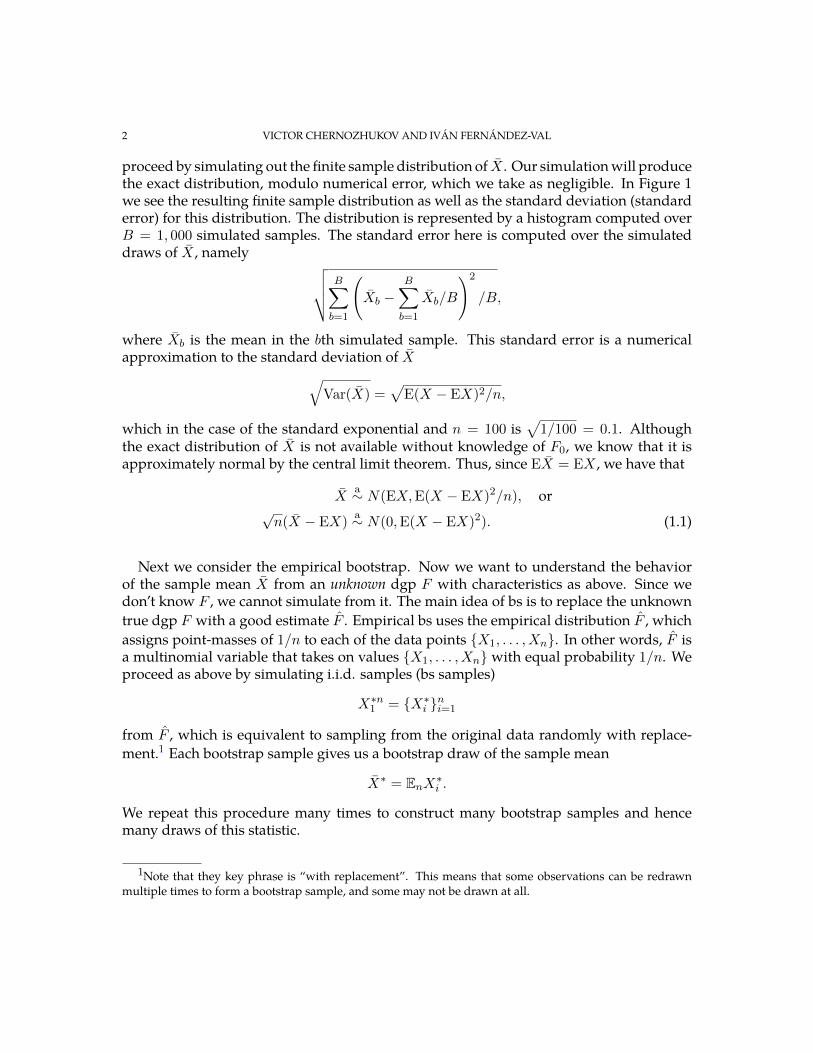
proceed by simulating out the finite sample distribution of X . Our simulation will produce the exact distribution, modulo numerical error, which we take as negligible. In Figure 1 we see the resulting finite sample distribution as well as the standard deviation (standard error) for this distribution. The distribution is represented by a histogram computed over B = 1, 000 simulated samples. The standard error here is computed over the simulated draws of X , namely �

B �B

¯ ¯Xb − Xb/Bb=1 b=1

2

/B,

where Xb is the mean in the

�bth simulated sample. This standard error is a numerical

approximation to the standard deviation of X Var(X ¯) = E(X − EX)2/n,

which in the case of the standard exponential

and n = 100 is 1/100 = 0.1. Although

the exact distribution of X is not available without knowledge of F0, we know that it is approximately normal by the central limit theorem. Thus, since

¯EX = EX , we have that

¯ aX ∼ N(EX, E(X − EX)2/n), or

√ ¯ a

n(X − EX) ∼ N(0, E(X − EX)2). (1.1)

Next we consider the empirical bootstrap. Now we want to understand the behavior of the sample mean X from an unknown dgp F with characteristics as above. Since we don’t know F , we cannot simulate from it. The main idea of bs is to replace the unknown true dgp F with a good estimate F . Empirical bs uses the empirical distribution F , which assigns point-masses of 1/n to each of the data points {X1, . . . , Xn}. In other words, F is a multinomial variable that takes on values {X1, . . . , Xn} with equal probability 1/n. We proceed as above by simulating i.i.d. samples (bs samples)

X ∗n = {Xi∗ }n

1 i=1

from F , which is equivalent to sampling from the original data randomly with replace­ment.1 Each bootstrap sample gives us a bootstrap draw of the sample mean

X∗ X ∗ = En i .

We repeat this procedure many times to construct many bootstrap samples and hence many draws of this statistic.

1Note that they key phrase is “with replacement”. This means that some observations can be redrawn multiple times to form a bootstrap sample, and some may not be drawn at all.

L5 3

histogram for true draws

values of statistic

Fre

quen

cy

0.8 0.9 1.0 1.1 1.2 1.3

040

8014

0

se= 0.0966

histogram for BS draws

values of statistic

Fre

quen

cy

0.8 0.9 1.0 1.1 1.2 1.3

040

8014

0

se= 0.0943

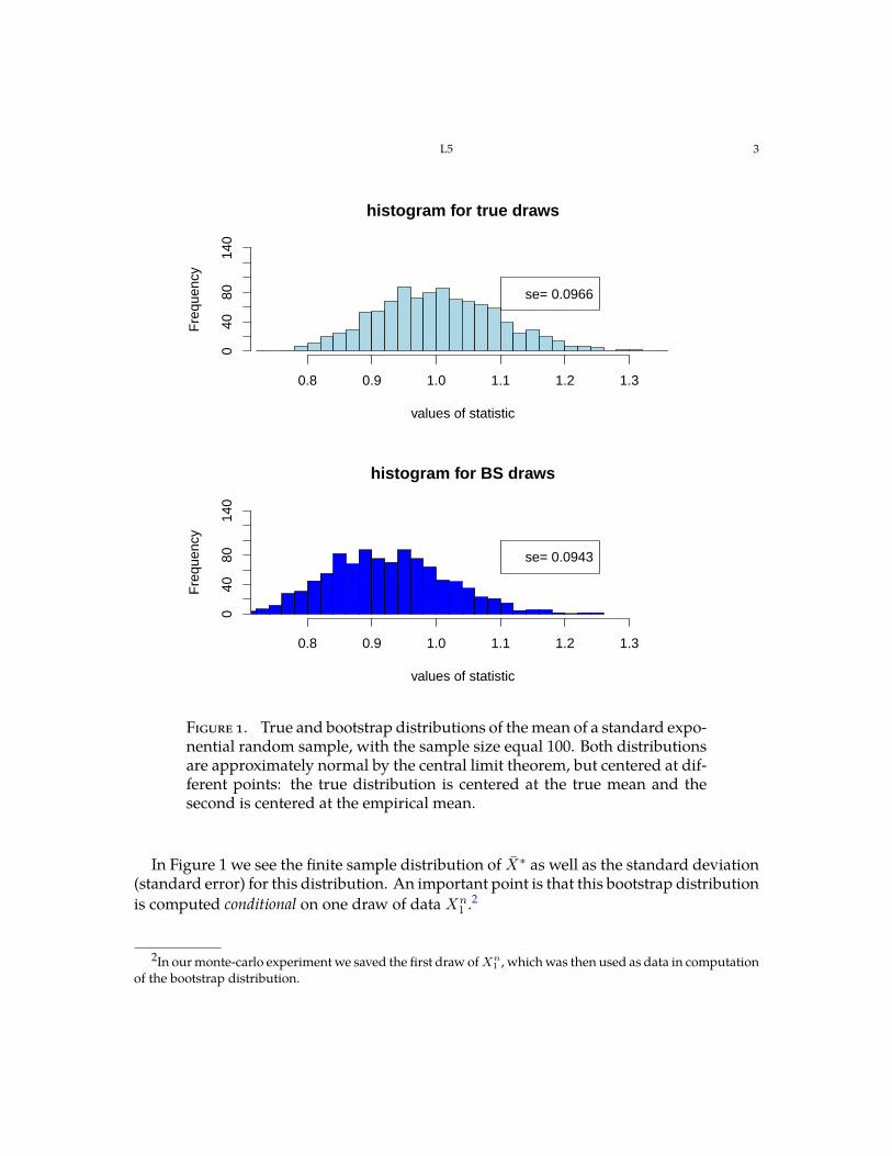
Figure 1. True and bootstrap distributions of the mean of a standard expo­nential random sample, with the sample size equal 100. Both distributions are approximately normal by the central limit theorem, but centered at dif­ferent points: the true distribution is centered at the true mean and the second is centered at the empirical mean.

¯In Figure 1 we see the finite sample distribution of X∗ as well as the standard deviation (standard error) for this distribution. An important point is that this bootstrap distribution is computed conditional on one draw of data X1

n.2

2In our monte-carlo experiment we saved the first draw of X1 n, which was then used as data in computation

of the bootstrap distribution.

�

4 VICTOR CHERNOZHUKOV AND IV AN´ FERNANDEZ- ´ VAL

X∗We note that not only the standard deviations of the bootstrap draws and actual draws X look very similar, but also the overall distribution of bootstrap draws X∗ and

¯actual draws X look very similar. This is not a coincidence.

¯The mean of the bootstrap distribution of X∗ is n

¯E(X∗ | X1 n) = Xi/n = X.

i=1 ¯Similarly, the standard deviation of the bootstrap distribution of X∗ is

X∗ ¯Var( ¯ | Xn) = En(Xi − X)2/n,1

which is simply the root of the empirical variance scaled by n. By the law of large numbers and some simple calculations,

¯En(Xi − X)2 →P E(X − EX)2 , we have that the ratio of bootstrap standard error and the actual standard error converges in probability to 1. Thus, the similarity of the computed standard errors was not a coin­cidence. Of course, we did not need the bootstrap to compute the standard errors of a sample mean, but we will need it very soon for less tractable cases.

¯We can approximate the exact distribution of X∗, conditional on the data, by simulation. Moreover, it is also approximately normal in large samples. By the central limit theorem

¯1) We see that the approximate distributions of n(X∗ − and n( ¯

and the law of large numbers,

X∗ | Xn ∼ N( ¯ (Xi − X)2/n),1 X, Ena (1.2) a∼ N( X, E(X − EX)2/n) or

√ n(X∗ − X) | Xn ∼ N(0, En(X − X)2)¯ ¯

1 a (1.3) a∼ N(0, E(X − EX)2).

Thus,

√ √ X) | Xn X − EX),1

¯namely N(0, En(Xi − X)2) and N(0, E(X − EX)2), are indeed close. 2) This means that their finite-sample distributions must be close.

We summarize the discussion of empirical bootstrap of the sample mean diagrammati­cally:

world dgp sample statistic approximate distribution √ areal F0 X1

n X n(X − EX) ∼ N(0, E(X − EX)2)√ aˆ X∗n X∗ ¯ ¯bootstrap F n(X∗ − X) | Xn ∼ N(0, En(Xi − X)2).1 1

∑√ √

L5 5

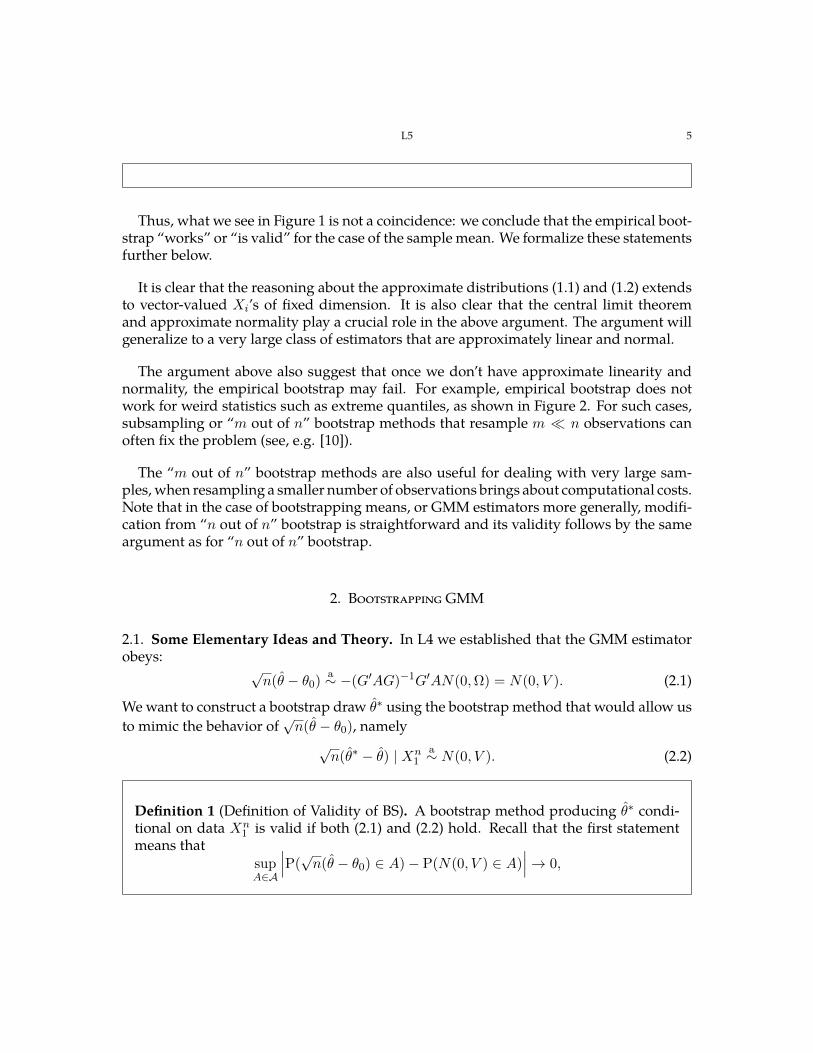
Thus, what we see in Figure 1 is not a coincidence: we conclude that the empirical boot­strap “works” or “is valid” for the case of the sample mean. We formalize these statements further below.

It is clear that the reasoning about the approximate distributions (1.1) and (1.2) extends to vector-valued Xi’s of fixed dimension. It is also clear that the central limit theorem and approximate normality play a crucial role in the above argument. The argument will generalize to a very large class of estimators that are approximately linear and normal.

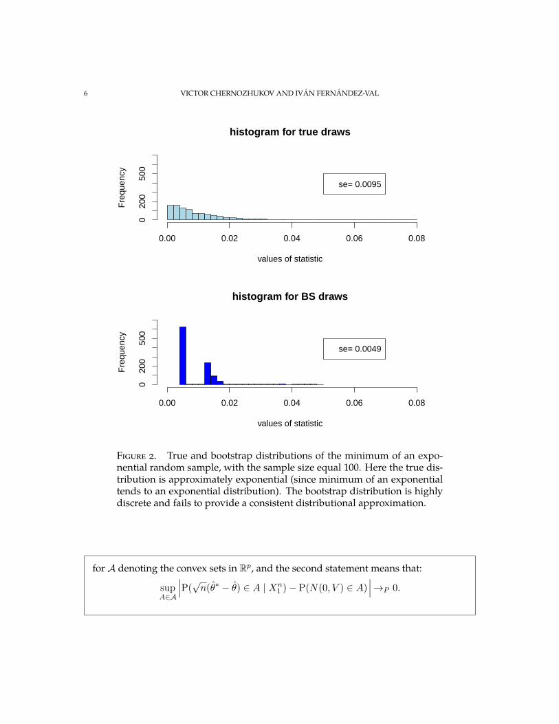
The argument above also suggest that once we don’t have approximate linearity and normality, the empirical bootstrap may fail. For example, empirical bootstrap does not work for weird statistics such as extreme quantiles, as shown in Figure 2. For such cases, subsampling or “m out of n” bootstrap methods that resample m « n observations can often fix the problem (see, e.g. [10]).

The “m out of n” bootstrap methods are also useful for dealing with very large sam­ples, when resampling a smaller number of observations brings about computational costs. Note that in the case of bootstrapping means, or GMM estimators more generally, modifi­cation from “n out of n” bootstrap is straightforward and its validity follows by the same argument as for “n out of n” bootstrap.

2. Bootstrapping GMM

2.1. Some Elementary Ideas and Theory. In L4 we established that the GMM estimator obeys:

a√ n(θ − θ0) ∼ −(G'AG)−1G'AN(0, Ω) = N(0, V ). (2.1)

We want to construct a bootstrap draw θ∗ using the bootstrap method that would allow us to mimic the behavior of

√ n(θ − θ0), namely

√ an(θ∗ − θ) | Xn ∼ N(0, V ). (2.2)1

Definition 1 (Definition of Validity of BS). A bootstrap method producing θ∗ condi­tional on data Xn is valid if both (2.1) and (2.2) hold. Recall that the first statement 1 means that

sup P( √ n(θ − θ0) ∈ A) − P(N(0, V ) ∈ A) → 0,

A∈A

6 VICTOR CHERNOZHUKOV AND IV AN´ FERNANDEZ- ´ VAL

histogram for true draws

values of statistic

Fre

quen

cy

0.00 0.02 0.04 0.06 0.08

020

050

0

se= 0.0095

histogram for BS draws

values of statistic

Fre

quen

cy

0.00 0.02 0.04 0.06 0.08

020

050

0

se= 0.0049

Figure 2. True and bootstrap distributions of the minimum of an expo­nential random sample, with the sample size equal 100. Here the true dis­tribution is approximately exponential (since minimum of an exponential tends to an exponential distribution). The bootstrap distribution is highly discrete and fails to provide a consistent distributional approximation.

for A denoting the convex sets in Rp, and the second statement means that: √

sup P( n(θ∗ − θ) ∈ A | X1 n) − P(N(0, V ) ∈ A) →P 0.

A∈A

∣∣∣ ∣∣∣

L5 7

Note that by the triangle inequality this definition implies the following “natural” defi­nition:

√ √ sup P( n(θ∗ − θ) ∈ A | X1

n) − P( n(θ − θ0) ∈ A) →P 0. A∈A

The previous definition however emphasizes the link with approximate normality, which is key to demonstrating that the empirical bootstrap works.

2.2. A Quick BS Method for GMM. A computationally quick way to bootstrap GMM is to bootstrap the average score appearing in the linear approximation to GMM. Recall that we obtained

√ n(θ − θ0) = −(G ' AG)−1G ' A

√ nEnZi +oP (1),

vector mean

where Zi = g(Xi, θ0). Thus GMM is approximately a sample mean over the scores Zi times a fixed matrix −(G ' AG)−1G ' A.

Thus we could simply bootstrap the scores Zi’s: Indeed, let Z∗n denote the empirical 1 bootstrap draws from the sample Zn, and define the bootstrap draw θ∗ via the relation: 1

¯√ n(θ∗ − θ) = −(G ' AG)−1G ' A

√ nEn(Zi

∗ − Z), that is,

θ∗ = θ − (G ' AG)−1G ' AEn(Z ∗ − Z).i

11

By the central limit theorem, law of large numbers, and smoothness of the Gaussian law we have the following properties:

√ anEn(Z ∗ − Z) | Zn ∼ N(0, Ωn)i 1

a∼ N(0, Ω),

where Ωn = En(Zi − Z)(Zi − Z) ' and Ω = E(Z − EZ)(Z − EZ) ' .3 This reasoning implies that our quick bs method is valid:

√ an(θ∗ − θ) | Xn ∼ −(G ' AG)−1G ' AN(0, Ω) = N(0, V ).1

3Here the first and second approximations formally mean that:

P( ) ∈ A | Xn) − P(N(0, Ωn) ∈ A | Xn →P √ ∗ Z∗ nEn(Z − ) 0,sup i

A∈A

1

P(N(0, Ωn) ∈ A | Xn

where A denotes the convex sets in Rp.

) − P(N(0, Ω) ∈ A) →P 0,sup

A∈A

8 VICTOR CHERNOZHUKOV AND IV AN´ FERNANDEZ- ´ VAL

In practice we need to replace G, A, and Zi’s with consistent estimators G, A, and Zi = g(Xi, θ) such that

G− G →P 0, A− A →P 0, Enlg(Xi, θ) − g(Xi, θ0)l2 →P 0,

and then just define the bootstrap draws via the relation:

¯√ n(θ∗ − θ) = −(G' AG)−1G' A

√ nEn(Z

∗ − Z).i

Note that here we are bootstrapping the estimated scores. We can then arrive at the fol­lowing conclusion.

Theorem 1 (Validity of Quick BS for GMM). Under regularity conditions, the quick boot­strap method is valid. That is, the quick bootstrap method approximately implements the normal distributional approximation for the GMM estimator. Moreover, the bootstrap variance estima­tor V = E[(θ∗ − θ)(θ∗ − θ) ' | X1

n] is consistent, namely that V − V →P 0.

2.3. A Slow BS Method for GMM. There is also a slow bs method for GMM. Here we just bootstrap the whole procedure.

Let X1 ∗, ..., X∗ denote the bootstrap sample. Let g∗(θ) = Eng(Xi

∗, θ) − g(θ), and n

θ∗ ∈ arg min g∗ (θ) ' A∗ g∗ (θ). θ∈Θ

Here A∗ denote the estimator of A obtained using X1 ∗, ..., X∗ .n

Then we might think that under regularity conditions we would have the linearization

¯√ n(θ∗ − θ) = −(G' AG)−1G' A

√ nEn(Z

∗ − Z) + oP (1),i

and then this is first-order equivalent to the quick bs method for GMM. This reasoning suggests the following result.

Theorem 2 (Validity of Slow BS for GMM). Under regularity conditions, e.g. those listed in [6], the slow bootstrap method above is valid. That is, the slow bootstrap method approximately implements the normal distributional approximation for the GMM estimator. Moreover, under appropriate strengthening of regularity conditions, see e.g. [9], bootstrap variance estimator V = E[(θ∗ − θ)(θ∗ − θ) ' | X1

n] is consistent, namely that V − V →P 0.

�

L5 9

Formal proofs of these results are beyond the scope of these lectures, but they can be found in the theoretical literature.

3. Algorithmic Details and Examples of Use

A basic use of bootstrap is for estimation of standard errors and construction of the confidence regions.

The following algorithm constructs estimates of the standard errors.

(1) Obtain many bootstrap draws θ∗(j) of the estimator θ, where the index j = 1, . . . , B enumerates the bootstrap draws.

(2) Compute the bootstrap variance estimator B

ˆ (θ∗(j) − ˆ θ ∗(j) − θ) ' V /n = B−1 θ)(ˆ . j=1

Report sk = ( Vkk/n)1/2 as standard errors for θk for k = 1, . . . d.

(3) An alternative is to report standard errors based on the interquartile ranges: sk = [ck(.75) − ck(.25)]/(Φ−1(.75) − Φ−1(.25)), k = 1, . . . d,

∗(j)where ck(a) = a-quantile of {θ , j = 1, ..., B} and Φ−1 is the quantile function k of the standard normal distribution Φ.

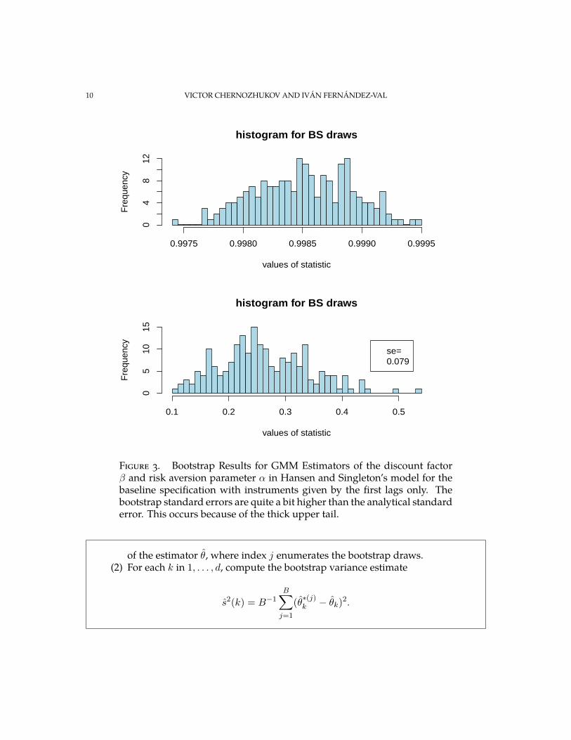
We illustrate the performance of bootstrap for GMM using the empirical example of L4. Here we focus on bootstrapping the 2-step GMM estimator for the first specification that we estimated. We can mechanically treat the data in that example as i.i.d., because the asymptotic distribution is the same as if we had i.i.d. sampling due to scores being an uncorrelated sequence. We show the histograms of the bootsrap draws θ∗ = (β∗ , α∗) for the estimator.

The following algorithm constructs a simultaneous confidence region (rectangle) for all components of θ0.

(1) Obtain many bootstrap draws

θ∗(j), j = 1, . . . , B

∑

�

10 VICTOR CHERNOZHUKOV AND IV AN´ FERNANDEZ- ´ VAL

histogram for BS draws

values of statistic

Fre

quency

0.9975 0.9980 0.9985 0.9990 0.9995

04

812

histogram for BS draws

values of statistic

Fre

quency

0.1 0.2 0.3 0.4 0.5

05

10

15

se=

0.079

Figure 3. Bootstrap Results for GMM Estimators of the discount factor β and risk aversion parameter α in Hansen and Singleton’s model for the baseline specification with instruments given by the first lags only. The bootstrap standard errors are quite a bit higher than the analytical standard error. This occurs because of the thick upper tail.

of the estimator θ, where index j enumerates the bootstrap draws. (2) For each k in 1, . . . , d, compute the bootstrap variance estimate

B

s2(k) = B−1 (θ∗(j) − θk)2 .k

j=1

∑

L5 11

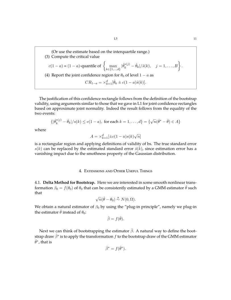
(Or use the estimate based on the interquartile range.) (3) Compute the critical value

| ∗(j) − ˆc(1 − a) = (1 − a)-quantile of max θ θk|/s(k), j = 1, . . . , B .kk∈{1,...,d}

(4) Report the joint confidence region for θ0 of level 1 − a as dCR1−a = ×k=1[θk ± c(1 − a)s(k)].

The justification of this confidence rectangle follows from the definition of the bootstrap validity, using arguments similar to those that we gave in L1 for joint confidence rectangles based on approximate joint normality. Indeed the result follows from the equality of the two events:

√∗(j){|θ − θk|/s(k) ≤ c(1 − a), for each k = 1, . . . , d} = { n(θ∗ − θ) ∈ A}k

where √dA = ×k=1[±c(1 − a)s(k) n]

is a rectangular region and applying definitions of validity of bs. The true standard error s(k) can be replaced by the estimated standard error s(k), since estimation error has a vanishing impact due to the smothness property of the Gaussian distribution.

4. Extensions and Other Useful Things

4.1. Delta Method for Bootstrap. Here we are interested in some smooth nonlinear trans­formation β0 = f(θ0) of θ0 that can be consistently estimated by a GMM estimator θ such that

a√ n(θ − θ0) ∼ N(0, Ω).

We obtain a natural estimator of β0 by using the ”plug-in principle”, namely we plug-in the estimator θ instead of θ0:

β = f(θ).

Next we can think of bootstrapping the estimator β. A natural way to define the boot­strap draw β∗ is to apply the transformation f to the bootstrap draw of the GMM estimator θ∗, that is

β∗ = f(θ∗ ).

12 VICTOR CHERNOZHUKOV AND IV AN´ FERNANDEZ- ´ VAL

Bootstrapping smooth functionals of vector means provides a valid distributional approximation, namely that √ √a an(β − β0) ∼ N(0, Vf ) and n(β∗ − β) | Xn ∼ N(0, Vf ), Vf = \f(θ0)Ω\f(θ0) ' .1

The approximate distribution of β is obtained by the delta-method:

where θ stands for a point on the line connecting θ and θ0 and Ω is the variance of n(ˆ

√ n(β − β0) = \f(θ)

√ n(θ − θ0)

= [\f(θ0) + oP (1)] √ n(θ − θ0)

a∼ \f(θ0)N(0, Ω) = N(0, Vf ), Vf = \f(θ0)Ω\f(θ0) ' ,

√ θ −

θ0). Here we require that \f(θ0) to have singular values bounded away from zero, since otherwise the normal approximation here would be poor.

Then we can give a reasoning similar to that used above: conditional on the data X1 n,

√ n(β∗ − β) = \f(θ∗ )

√ n(θ∗ − θ)

[\f(ˆ√ n(θ∗ − ˆ= θ) + oP (1)] θ)

a∼ \f(θ0)N(0, Ω) = N(0, Vf ), Vf = \f(θ0)Ω\f(θ0) ' ,

where θ∗ is a point on the line connecting θ∗ and θ and Ω is the variance of √ n(θ − θ0).

4.2. Bootstrapping Dependent Data. The idea is to divide data in blocks, where depen­dence is preserved within blocks, and then bootstrap the blocks, treating them as inde­pendent units of observations. Here we provide a brief description of the construction of the bootstrap samples. We refer to [7] for assumptions and theoretical results.

Let’s assume that we want to draw a bootstrap sample from a stationary and strongly ¯missing sequence X1

n. For example, Xi = −(G' AG)−1G' A(Zi − Z) in the quick bs for GMM, whereas Xn is the original sample in the slow bs for GMM. The blocks of data 1

jcan be overlapping or non-overlapping. We focus on the non-overlapping case. Let X = (Xi, Xi+1, . . . , Xj ) for i < j, and s be the block size. We assume for simplicity that n = sb for some integer b. We construct the bootstrap sample X1

∗, . . . , X∗ by stacking b blocks ran-n domly drawn from {X1

s, Xs2 } with replacement. The block size s shoulds+1, . . . , Xsb s(b−1)+1

i

L5 13

be chosen such that s → ∞ and s = O(n1/3) as n → ∞. For GMM problems, [4] and [8] recommend setting the block size equal to the trimming parameter in the estimation of Ω.4

Notes

The bootstrap method was introduced by Bradley Efron in [2]. Pioneer work in the development of asymptotic theory for the bootstrap includes [1] and [3]. Hall studied the higher order properties of the bootstrap in [5]. For applications to Econometrics, including GMM, see Horowitz’s chapter in Handbook of Econometrics in [7].

5. Problems

Problem 1. Explain in exactly 1 page why empirical bootstrap works for the sample mean and why empirical bootstrap works for GMM ( you can use “quick” bootstrap for this purpose).

Problem 2. Obtain bootstrap standard errors for the Hansen and Singleton example ana­lyzed in the previous lecture. Obtain a confidence interval for the risk aversion parameter in that example.

Problem 3. Obtain joint confidence bands via empirical bootstrap for the four treatment effects in the Pennsylvania re-employment experiment in L1.

Problem 4. Modify algorithms in Section 3 for the case of “m out of n” bootstrap. Be careful with scaling. Present a brief reasoning similar to that in Section 2 arguing that “m out of n” bootstrap will also work for GMM.

References

[1] Peter J. Bickel and David A. Freedman. Some asymptotic theory for the bootstrap. Ann. Statist., 9(6):1196–1217, 1981.

[2] B. Efron. Bootstrap methods: another look at the jackknife. Ann. Statist., 7(1):1–26, 1979.

[3] Evarist Gine and Joel Zinn. Bootstrapping general empirical measures. Ann. Probab., 18(2):851–869, 1990.

4Recall from L4 that the Newey-West estimator of Ω is L n −£L L

ˆ Σ� ˆ ˜ ˜Ω = Σ0 + ω£L (Σ£ + ˆ£ ), Σ£ = g(Xi , θ)g(Xi +£ , θ)/n, ω£L = 1 − e/(L + 1),

£ =1 i =1

where θ is a preliminary estimator of θ0 and L is the trimming parameter.

14 VICTOR CHERNOZHUKOV AND IV AN´ FERNANDEZ- ´ VAL

histogram for BS draws

values of statistic

Fre

quency

0.9982 0.9984 0.9986 0.9988 0.9990

010

20

30

histogram for BS draws

values of statistic

Fre

quency

0.15 0.20 0.25 0.30 0.35 0.40 0.45

010

20

30

Figure 4. (Independent) Bootstrap Results for GMM Estimators of α and β in Hansen and Singleton’s model for the baseline specification with in­struments given by the first lags only.

[4] F. G¨ unsch. Second-order correctness of the blockwise bootstrap for otze and H. R. K stationary observations. Ann. Statist., 24(5):1914–1933, 1996.

[5] Peter Hall. The bootstrap and Edgeworth expansion. Springer Series in Statistics. Springer-Verlag, New York, 1992.

[6] Peter Hall and Joel L. Horowitz. Bootstrap critical values for tests based on generalized-method-of-moments estimators. Econometrica, 64(4):891–916, 1996.

[7] Joel L. Horowitz. The bootstrap. In James J. Heckman and Edward Leamer, editors, Handbook of Econometrics. Volume 5. Elsevier: North-Holland, 2001.

L5 15

[8] Atsushi Inoue and Mototsugu Shintani. Bootstrapping {GMM} estimators for time series. Journal of Econometrics, 133(2):531 – 555, 2006.

[9] Kengo Kato. A note on moment convergence of bootstrap M -estimators. Statist. De­cisions, 28(1):51–61, 2011.

[10] Dimitris N. Politis, Joseph P. Romano, and Michael Wolf. Subsampling. Springer Series in Statistics. Springer-Verlag, New York, 1999.

MIT OpenCourseWarehttps://ocw.mit.edu

14.382 EconometricsSpring 2017

For information about citing these materials or our Terms of Use, visit: https://ocw.mit.edu/terms.