1402.1255

Option Pricing, Historical Volatility and Tail Risks

Samuel E. VazquezBaruch College, CUNY

[email protected]

February 7, 2014

Abstract

We revisit the problem of pricing options with historical volatility estimators. We do this in thecontext of a generalized GARCH model with multiple time scales and asymmetry. It is argued that thereason for the observed volatility risk premium is tail risk aversion. We parametrize such risk aversionin terms of three coefficients: convexity, skew and kurtosis risk premium. We propose that optionprices under the real-world measure are not martingales, but that their drift is governed by such tailrisk premia. We then derive a fair-pricing equation for options and show that the solutions can bewritten in terms of a stochastic volatility model in continuous time and under a martingale probabilitymeasure. This gives a precise connection between the pricing and real-world probability measures,which cannot be obtained using Girsanov Theorem. We find that the convexity risk premium, notonly shifts the overall implied volatility level, but also changes its term structure. Moreover, the skewrisk premium makes the skewness of the volatility smile steeper than a pure historical estimate. Wederive analytical formulas for certain implied moments using the Bergomi-Guyon expansion. Thisallows for very fast calibrations of the models. We show examples of a particular model which canreproduce the observed SPX volatility surface using very few parameters.

1 Introduction

Most option pricing models are written directly in the martingale or pricing probability measure[1]. Such models usually have a significant number of parameters which need to be fitted to thevolatility surface. In the end, such parameters will show strong time dependency, invalidating theinitial assumptions of the model. Moreover, the final values of the parameters have little physicalsignificance, and so there is no notion of a “fair” option price. We think of this as a fit-only approach,which in our opinion is best done in the context of parametric smile models such as SSVI [2].

1

arX

iv:1

402.

1255

v1 [

q-fi

n.PR

] 6

Feb

201

4

On the other hand, there is another stream of literature which studied the volatility surface pro-duced by GARCH volatility forecasts [3, 4, 5, 6]. However, here one runs into another problem: whatis the relation between the real-world and the pricing or martingale probability measure? One solu-tion is to leave free some of the GARCH parameters so they can be fitted to the volatility surface.However, this puts us back into the fit-only approach without any understanding of the physical mean-ing of these parameters. Worst, the GARCH models are written in discrete time, and hence requiretime-consuming Monte Carlo simulations in order to find the optimal parameters.

An early attempt to find a direct relation between the pricing and real-world measure in the contextof GARCH models is found in [3]. This approach assumes that the one-period expected variance, isthe same in both probability measures. However, this assumption is wrong as we will show in thispaper. In fact, due to tail risks, there should be a significant premium paid to the short gammatrader even for one-day returns. In other approaches, such as [4], the authors start by modeling logreturns in discrete time and define the pricing measure by requiring simple returns to be a martingale.However, as we will show in this paper, the volatility risk premium has nothing to do with the driftof the underlying. In fact, option prices are very insensitive to drifts and the underlying can very wellbe a martingale in both the real-world and pricing measure. A notable exception to this literaturestream is [7, 8], which uses a price kernel approach to connect both probability measures. We believethere is an interesting connection between their approach and ours, but we will leave this for futurework.

In this article we introduce a new approach to option pricing. Our goal is to use historical volatilityestimators, while introducing risk premia which will allow to fit the volatility surface. In fact, onlythe risk premia needs to be fitted to the option prices. The rest of the parameters will be determinedusing the time series of the underlying. We will show that most of the features of the volatility surfacecan be explained using a good volatility forecast and only three risk premia. We will assume that therisk premia are constant. This is not true in practice, but a generalization is possible and will be leftfor future work. We will argue that the risk premium parameters we introduce are related to tail riskaversion, and come from the fact that option traders mark to market their books in discrete time andhave limited capital.

We will begin by working in discrete time, but assume the time step to be small enough so thatwe can expand option prices to second order in variations of the stochastic variables. This is whatmost option traders do in practice. Moreover, as most practitioners know, only the first few Greekscan be traded in the market due to liquidity constraints. This approximation will allow us to make aconnection with the more familiar continuous time stochastic volatility models.

We define tail risk as a typical large move of the underlying, not necessarily a catastrophic “Black-Swan” event [9]. However, we do not assign probabilities to such events. In practice, all marketparticipants have limited capital, and must limit their leverage so that they can withstand such tailevents. In fact, most brokers determine margin requirement precisely this way, using stress testing.What does this mean in practice? Suppose you are a trader who is short gamma. Under a large moveof the underlying price S, you face a potentially large loss of size: lim|δS|→∞ δP = −ΓδS2, whereΓ > 0 is the net gamma exposure. This is an unhedgable tail risk! In other words, there is a large tail

2

risk asymmetry between a long-volatility and a short-volatility position. The short volatility tradermust then put aside more capital than the long volatility counter-party. This is a cost of carry and soit is only fair that the short-volatility trader gets compensated by having a non-zero drift in his/herportfolio: E[δP ] > 0. This very simple argument is the basis of our option pricing approach. In anutshell, we propose that in the real-world measure, the drift of option returns is governed by theprices of tail risk.

We will restrict ourselves to a class of GARCH models with asymmetry and multiple time scales.However, our methodology can be applied to more general models, even those that include high-frequency volatility estimators [10]. We derive a generalized Black-Scholes equation under the real-world measure. Using Feynman-Kac theorem, we map the solutions to this equation to a stochasticvolatility model in continuous time and under a martingale probability measure. This gives a precisemapping from the real-world to the pricing measure. However, this connection cannot be obtainedusing the standard Girsanov transformation.

Using the results of Bergomi and Guyon [11], we derive approximate formulas for certain im-plied moments up to second order in the volatility of volatility (vol-of-vol). These moments can becompared to the corresponding strip of options for fast calibration. Each risk premium is calibratedindependently. In particular, we show that we can get the convexity/gamma risk premium by fittingthe variance swap term structure. Moreover, the skew and kurtosis risk premia are obtained by fittingsimilar strip of options. Once the risk premia are calibrated, one can generate full volatility surfacesusing Monte Carlo simulations. We show that the volatility surfaces obtained this way are close towhat we observe in the market.

We should stress that the goal of this paper is not to provide a comparative study of GARCHmodels or best estimation techniques. Our purpose is simply to introduce a new pricing methodologyand give some examples. Therefore, we will not attempt to compare the fit quality of different models.

In section 2 we will make the tail risk argument more precise and define the risk premia. In section3 we study in detail the GARCH(1,1) model which serves to illustrate the main ideas. In section 4 wegeneralize the GARCH model to include asymmetry and multiple time scales. In section 5 we deriveapproximate formulas for certain implied moments of the underlying returns. In section 6 we explainhow the calibration is done using SPX option data. Moreover, we give examples of the volatilitysurfaces obtained from a particular GARCH model. We conclude in section 7.

1.1 Notation

We denote the price of the underlying asset by St, where t is time measured in years. As usual, weassume that St is the forward price, so that we can ignore dividends and interest rates. When workingin discrete time we take a one day time step: δt = 1/252 (in years). Simple returns will be denotedby

δSt := St − St−δtIn general, time subscripts denote stochastic time dependence while parenthesis denote smooth timedependence. For example, xt(T ) is a smooth function of T for fixed t. Moreover, all stochastic

3

processes of the form xt are t-measurable in the sense that they depend on information up to time t.The underlying return will be decomposed as follows:

rt :=δStSt−δt

=√δt νt−δtεt

where εt is a i.i.d. noise with zero mean and unit standard deviation, and νt is the realized annualizedvariance. Note that we take the underlying to be a martingale under the real-world measure. However,adding a drift or taking log-returns instead has a negligible effect on the parameters of the model.We also find little evidence for skewness in the distribution of εt. Therefore, we will assume that thedistribution of εt is symmetric.

We will make ample use of exponential moving averages or EMAs. Our definition is the following:

EMAL[xt] =

(1− 1

L

)EMAL[xt−δt] +

1

Lxt (1)

where L is the time scale of the EMA in days, and xt is some random process.The real-world probability measure is denoted by P. The notation Et[xT ] for T ≥ t means con-

ditional expectation with information up to time t. The pricing measure will be denoted by P? withsimilar notation for the conditional expectation: E?t [xT ].

2 Tail Risks

The tail risk of an option trader follows from the non-linear dependency of options on the movementsof the underlying asset. We consider tail scenarios parametrized by the normalized return εt. Forexample, εt = ±3 is a “3-sigma” scenario. Moreover, we use the notation lim|εt|→∞ to denote alarge underlying move (not literally infinite). Basically, we think about typical scenarios of 3-5 sigma.These are not Black Swan events, as they happen quite often. However, they are large enough tocause substantial losses to option traders and trigger margin calls.

Suppose we have a portfolio P (2) with some gamma exposure such that, under a tail event wehave:

lim|εt|→∞

δP(2)t = ε2t (2)

where the superscript in P(2)t indicates the asymptotic quadratic dependency on εt. As we discussed

in the introduction, a trader with a short position in P (2) will be asked by the broker to put moremargin than the one with a long position. This is a cost of carry, because he/she could be investingthis money somewhere else. In order to compensate this trader, the profits and losses (P&L) of P (2)

must have a drift in the real-world measure:

Et[δP

(2)t+δt

]= −λ2 (3)

4

where we expect λ2 > 0 on average. We call λ2 the convexity or gamma risk premium. Note that wedo not have to know any details about this portfolio, but only its asymptotic exposure to ε. In fact,the key assumption of this paper is that the form of such portfolio does not matter, and that anyother portfolio, say P (2), with the same tail risk will have the same drift. In other words, derivativemarkets only price tail risks and not “daily” variance.

A simple example of a portfolio with gamma exposure is the front VIX future contract. In figure 1we compare the cumulative P&L of the front short VIX contract with those of the front long SPMINI.Both P&Ls have been risk managed so that they have the same daily risk in a scale of 20 days1.We can clearly see that the VIX future has a greater risk premium than the SPMINI for the samedaily risk. However, it also has larger draw-downs. In figure 2 we show the residual VIX future P&Lconditioned on the SPMINI future P&L2. It is clear that the short VIX future has a gamma componentthat causes quadratically large losses for large movements of the SPMINI. This is the reason for theextra premium!

20052006

20072008

20092010

20112012

20132014

Date

50

0

50

100

150

200

Cum

ula

tive P

nL

VIX (0.96)

SPMINI (0.57)

Figure 1: Cumulative P&L of the front short VIX and long SPMINI futures. Each future has been risk-managedto maintain approximately one dollar of daily risk on a rolling scale of 20 days. The annualized Sharpe ratios areshown in parenthesis.

Now consider a portfolio P (3) such that,

lim|εt|→∞

δP(3)t = ε3t (4)

1More precisely, let Rt = Ft − Ft−δt be the daily P&L of the future contract. The risk managed P&L is given by

Rt = Rt/√

EMA20[R2t−δt].

2The residual P&L is defined by rVIX − βrSPMINI, where β := Cov[rVIX, rSPMINI]/Var[rSPMINI], where rVIX, rSPMINI arethe risk-managed PnLs of the VIX and SPMINI contracts respectively.

5

6 4 2 0 2 4 6

SPMINI PnL

2.0

1.5

1.0

0.5

0.0

0.5

1.0

1.5

2.0

E[V

IX P

nL

(resi

dual)

| SPM

INI PnL]

fit

data

Figure 2: Front short VIX future residual P&L conditioned on the front long SPMINI future P&L. The condi-tioning has been done by dividing the observations into 200 bins. We also show a quadratic polynomial fit forvisual clarity.

In equity markets, most traders are afraid of the left tail. This means that the trader with a longposition in P (3) is exposed to cubic losses under a large drawdown. In such markets one expects tosee a skew risk premium such that

Et[δP

(3)t+δt

]= λ3 (5)

where λ3 > 0 on average. In FX or certain commodity markets, we do not expect to see such riskpremium as market participants are equally afraid to both the left and right tail.

Note that this is a statement about risk aversion and not about the probability distribution of themarket. In fact, one can argue that nobody know the true real-world probability measure. However,all of us have capital requirements that become more stringent on downside equity markets (e.g. mostinvestors are long equities by definition).

Finally, we introduce a kurtosis risk premium:

lim|εt|→∞

δP(4)t = ε4t (6)

Et[δP

(4)t+δt

]= −λ4 (7)

where we expect λ4 > 0 on average.One can imagine higher moments, but as most option traders know, it is increasingly difficult to

get such exposures due to liquidity constraints. The higher the moment, the more we need to leveragethe option book and the less capacity there is for such strategy. Moreover, in the GARCH modelsstudied below, we do not get higher order exposures if we restrict ourselves to second-order Greeks.

6

The risk premia (λ2, λ3, λ4) will turn out to be the only parameters than need to be fitted to optionprices.

3 The GARCH(1,1) Model

In this section we study in detail the GARCH(1,1) model. This is the simplest model of the GARCHfamily and will serve to illustrate the main ideas. The goal of this section is to derive the pricingor martingale probability measure for this model using a tail risk argument. We begin by pricing avariance swap, and later move to price a general European contingency claim.

The GARCH(1,1) model is basically an EMA filter:

νt = ν(1− α) + αXt (8)

Xt =1

δtEMAL[r2t ] (9)

δXt+δt =1

L

(νtε

2t+δt −Xt

)(10)

where ν is the unconditional variance and α ∈ [0, 1] is a parameter that controls the strength of thevolatility autocorrelation.

3.1 Pricing a Variance Swap

Let’s now begin by pricing a variance swap contract with maturity date T . We denote the price ofsuch contract at time t by Vt(T ). At expiry our variance swap pays PT (T ) =

∑Nj=1 r

2t+jδt − Vt(T ),

where T = t+Nδt is the expiry date and N the number of days between t and T . Since it takes zerocapital to enter such contract, the P&L of the variance swap between time t and t+ δt is given by

δPt+δt(T ) = Vt+δt(T )− Vt(T ) + r2t+δt (11)

We now assume that the price Vt(T ) is a smooth function of time and the filter Xt, Vt(T ) := V (t,Xt).Moreover, note that the boundary condition is V (T,X) = 0. Up to second order in variations of Xand assuming a small enough time step δt we have,

δPt+δt(T ) ≈ ∂V

∂tδt+

∂V

∂XtδXt+δt +

1

2

∂2V

∂X2t

δX2t+δt + νtε

2t+δtδt (12)

This expansion will turn out to be exact in this case.We now look at the tail risks of the variance swap. Using Eqs. (2), (6) and (10) in Eq. (12), we

can decompose the asymptotic limit of the variance swap P&L as follows:

lim|εt+δt|→∞

δPt+δt(T ) = lim|εt+δt|→∞

[∂V

∂Xt

νtLδP

(2)t+δt + νtδtδP

(2)t+δt +

1

2

∂2V

∂X2t

ν2tL2δP

(4)t+δt

](13)

7

We should emphasize that since we want to consider a general solution V (t,X), we cannot comparethe different terms in Eq. (13) as we do not know the magnitude of the derivatives. In fact, for thevariance swap it turns out that V is a linear function of X and so the second derivative vanishes.

According to our argument in the previous section, any two portfolios with the same tail risksshould have the same drift. Therefore, using Eqs. (3) and (7) and the asymptotics given in Eq. (13),we conclude that the drift of the variance swap must be given by

Et [δPt+δt] = Et[δP

(2)t+δt

]( ∂V

∂Xt

νtL

+ νtδt

)+

1

2Et[δP

(4)t+δt

] ∂2V∂X2

t

ν2tL2

= −λ2(∂V

∂Xt

νtL

+ νtδt

)− λ4

2

∂2V

∂X2t

ν2tL2

(14)

This is the fair-value equation for the variance swap under the real-world probability measure. Moreexplicitly, we can write Eq. (14) as a PDE for V (t,X):

∂V

∂t+ θ [ν(1 + λ2)−X]

∂V

∂X+

1

2ξ2ν2

∂2V

∂X2+ (1 + λ2)ν = 0 (15)

where

ν = ν(1− α) + αX (16)

θ = (δtL)−1 (17)

ξ =

√m4 − 1 + λ4

L√δt

(18)

m4 = E[ε4] (19)

and the boundary condition is V (T,X) = 0. In writing Eq. (15) we have discarded a term quadraticin the drift of δX: Et[δX2

t+δt] ≈ (m4 − 1)ν2t /L2. We find that, empirically, this is a very good

approximation.Using Feynman-Kac formula, one can write the solution to Eq. (15) in terms of a continuous time

stochastic volatility process:

Vt(T ) = (1 + λ2)

∫ T

tE?t [νs]ds

νt = ν(1− α) + αXt

dXt = θ[νt(1 + λ2)−Xt]dt+ ξνtdZ?t

Note that the pricing probability measure P? is just a mathematical trick to solve Eq. (15). However,it is very useful in order to get analytical solutions. In fact, in this case the solution can be calculatedexplicitly:

Vt(T ) = Xτ + α(1 + λ2)(

1− e−θ′τ) Xt − X

θ′(20)

8

where the value of the filter Xt is given by Eq. (9) and

τ = T − tθ′ = θ[1− α(1 + λ2)]

X =ν(1− α)(1 + λ2)

1− α(1 + λ2)

Since Eq. (20) is linear in Xt, we can see that this is an exact solution to the variance swap price toall order in vol-of-vol. In fact, the solution only depends on the convexity or gamma risk premium.Therefore, by calibrating the variance swap term structure we can obtain the value of λ2. Moreover,notice how the gamma risk premium not only shifts the level of the varswap, but also changes theeffective mean-reversion time scale, which in turn changes the slope of the term structure.

Finally, note that the level of the implied expected variance is shifted from the historical one, evenat the smallest time step:

limδt→0

Vt(t+ δt)

δt= (1 + λ2)νt

where νt is given by the historical estimate of Eq. (8). This invalidates the assumption of [3], whoproposed that the one-period expected variance is the same in both the real-world and martingaleprobability measures.

3.2 Pricing Options

We now generalize the previous problem to price a Europen-style option C(t, S,X) with final payoffC(T, S,X) = g(S). For a delta-hedged option, the second order expansion reads:

δCt+δt ≈∂C

∂tδt+

∂C

∂XtδXt+δt +

1

2

∂2C

∂X2t

δX2t+δt +

1

2

∂2C

∂S2t

δS2t+δt +

∂2C

∂St∂XtδSt+δtδXt+δt (21)

where δCt+δt = δCt+δt − ∂C∂St

δSt+δt − rCtδt is the P&L of the self-financed and delta-hedged option,and r is the risk-free rate which we take to be constant. The tail risks now include a skew contributiondue to the cross term δSδX ∼ ε3. More precisely, we have:

lim|εt+δt|→∞

δCt+δt = lim|εt+δt|→∞

[νtL

∂C

∂XtδP

(2)t+δt +

ν2t2L2

∂2C

∂X2t

δP(4)t+δt +

S2t νtδt

2

∂2C

∂S2t

δP(2)t+δt

+

√δtν

3/2t StL

∂2C

∂St∂XtδP

(3)t+δt

](22)

Hence, the drift of the delta-hedged option is given by:

Et[δCt+δt] = −λ2(νtL

∂C

∂Xt+S2t νtδt

2

∂2C

∂S2t

)+ λ3

√δtν

3/2t StL

∂2C

∂St∂Xt− λ4

ν2t2L2

∂2C

∂X2t

(23)

9

which leads to the following PDE for the option price:

∂C

∂t− rC + θ [ν(1 + λ2)−X]

∂C

∂X+

1

2(1 + λ2)νS

2∂2C

∂S2+

1

2ξ2ν2S2 ∂

2C

∂X2+√

1 + λ2ρξν3/2S

∂2C

∂S∂X= 0

(24)where ν, θ and ξ are defined in Eqs. (16) - (18) and

ρ = − λ3√(1 + λ2)(m4 − 1 + λ4)

(25)

Using Feynman-Kac formula, we can write the solutions to Eq. (24) in terms of the followingstochastic process

Ct(T ) = e−r(T−t)E?t [g(ST )] (26)

dStSt

=√

(1 + λ2)νtdW?t (27)

νt = ν(1− α) + αXt (28)

dXt = θ(νt(1 + λ2)−Xt)dt+ ξνtdZ?t (29)

E?[dW ?t dZ

?t ] = ρdt (30)

As in the special case of the variance swap, the probability measure P? is the so-called martingaleor pricing measure. It is interesting to note that we have derived a direct connection between thereal-world and pricing measures parametrized by the three risk premia (λ2, λ3, λ4). These are theonly parameters that must be inferred from the option prices. The rest is completely determined byhistorical data, including the initial value of the EMA filter Xt.

Looking at Eq. (27) we notice how the convexity risk premium λ2 makes the implied volatilityhigher than the historical one (on average). Moreover, we can see that this risk premium cannotbe absorbed into the probability measure using a Girsanov transformation on (W ?, Z?). There is afundamental reason for this: the presence of λ2 comes from the fact that the option P&L is markedto market in discrete time. Another way to see this is that the underlying price is a martingale bothin the real-world and pricing measures. Therefore, the volatility risk premium has nothing to do withthe drift of the underlying. Many authors seem to confuse the volatility risk premium with the equityrisk premium. Those are two completely different quantities. In fact, there are many assets which donot have any obvious risk premium (e.g. FX rates or some commodities). However, their options stillshow a volatility risk premium. Therefore, any attempt to derive the pricing measure by putting amartingale condition on St is doomed to fail (see e.g. [3, 6]).

The skew risk premium λ3 makes the correlation between the spot and the volatility more negative.In fact, even if the underlying distribution is symmetric, we can still have non trivial implied leverageeffect due to the skew risk premium. Finally, the kurtosis risk premium makes the implied vol-of-volhigher than the historical estimate.

10

The stochastic process given by Eqs. (27) - (30) is well defined only if the risk premia obey thefollowing bounds:

λ2 > −1 (31)

λ4 ≥ −m4 + 1 +λ23

1 + λ2(32)

The second bound comes from the fact that we need |ρ| ≤ 1.

4 Including Asymmetry and Multiple Time Scales

There is a considerable number of studies that give evidence of multiple time scales in volatilityauto-correlations (see for example [12, 13, 14, 15, 16, 17, 18]) . In fact, it has been argued thatvolatility auto-correlations decay as a power law [18]. One problem with a power-law filter is thatit is non-Makovian. However, as shown in [19], one can always approximate a power law filter withmultiple exponentials. Hence, in this section we study a generalized GARCH models which is a linearcombination of EMA filters with different time scales.

Another stylized fact of volatility, is the so-called leverage effect [20]. In other words, for equityindices, negative returns tend to increase future volatility more than positive ones. In the context ofGARCH models, this is captured by adding a filter that depends only on past negative returns [21].Hence, we will study the following general class of models:

rt =√νt−δtεt

√δt (33)

νt =

N+M∑i=1

αiXit (34)

Xit =

1δtEMALi [r

2t ] for i = 1, . . . , N

2δtEMALi [r

2t 1rt<0] for i = N + 1, . . . , N +M

(35)

where∑N+M

i=1 αi = 1, δt = 1/252, rt = St/St−δt − 1 , and the i.i.d. noise term εt has zero mean andunit standard deviation. Note that we do not have constant unconditional variance in Eq. (34) as wedid in the simple GARCH(1,1) model. However, we can always take one of the time scales to infinity,say L1 →∞. This way we can recover the usual GARCH(1,1) model for example. In practice we willtake L1 = 1000 days. This way we avoid too much in-sample bias as we only use past observationsand we avoid having to fit the long term unconditional variance.

In order to find the pricing measure for this model, we can go over the same argument as in section

11

4. However, when expanding the option P&L we now will have the following new tail risks:

lim|εt|→∞

δXt ∝ ε2t1εt<0 (36)

lim|εt|→∞

δStδXt ∝ ε3t1εt<0 (37)

lim|εt|→∞

δX2t ∝ ε4t1εt<0 (38)

where δXt is one of the asymmetric filters. We can now imagine ideal portfolios, so that

lim|εt|→∞

δP(n)t = εnt 1εt<0

for n = 2, 3, 4. In order to avoid introducing more risk premia for our model, we will argue that inequity markets, investors are only afraid of large negative returns. In other words, they only valuedownside tail risk. Therefore, these new tail risks must have the same drift as the symmetric ones:

Et[δP(2)t+δt] = Et[δP

(2)t+δt] = −λ2 (39)


(3)t+δt] = λ3 (40)


(4)t+δt] = −λ4 (41)

where we used Eqs. (3), (5) and (7).In order to value an option, we assume as before that its price is a smooth function of time, the

spot and the filters: Ct(T ) = C(t, S,X). Expanding to second order in variations and taking intoaccount the tail risks as in the previous section, we get the following PDE:

∂C

∂t− rC +

∑i

θi[νδi −Xi

] ∂C∂Xi

+1

2(1 + λ2)νS

2∂2C

∂S2+

1

2

∑ij

ξiξjρijν2S2 ∂2C

∂Xi∂Xj

+√

1 + λ2∑i

ρiξiν3/2S

∂2C

∂S∂Xi= 0 (42)

12

where we have dropped terms quadratic in the drift of δXit and we have defined the following variables:

ν =∑i

αiXi (43)

θi = (Liδt)−1 (44)

δi =

1 + λ2 for i = 1, . . . , N

1 + 2λ2 for i = N + 1, . . . , N +M(45)

ξi =

√m4−1+λ4Li√δt

for i = 1, . . . , N√2m4−1+4λ4Li√δt

for i = N + 1, . . . , N +M(46)

ρi =

−λ3√

(1+λ2)(m4−1+λ4)for i = 1, . . . , N

2(m−3 −λ3)√(1+λ2)(2m4−1+4λ4)

for i = N + 1, . . . , N +M(47)

m−3 = E[ε31ε<0] (48)

m4 = E[ε4] (49)

Moreover, the correlation between the filters is one if both are symmetric or asymmetric (ρij = 1),but the correlation between a symmetric and asymmetric filter is:

ρij =m4 − 1 + 2λ4√

(m4 − 1 + λ4)(2m4 − 1 + 4λ4), (50)

for i ∈ 1, . . . , N , j ∈ N + 1, . . . , N +M.Using Feynan-Kac formula, we can relate the solutions of Eq. (42) to the following stochastic

volatility model:

Ct(T ) = e−r(T−t)E?t [g(ST )] (51)

dStSt

=√

(1 + λ2)νtdWt (52)

νt =∑i

αiXit (53)

dXit = θi[νtδi −Xi

t ]dt+ ξiνtdZit (54)

E?[dWtdZit ] = ρidt (55)

E?[dZitdZjt ] = ρijdt (56)

The Brownian motions can be decomposed into a few PCA factors as follows:

dZit =

ρ+dWt +√

1− ρ2+(√|ρ+−|dZt +

√1− |ρ+−|dZ+

t

)for i = 1, . . . , N

ρ−dWt +√

1− ρ2−(

sign(ρ+−)√|ρ+−|dZt +

√1− |ρ+−|dZ−t

)for i = 1 +N, . . . , N +M

(57)

13

where all Brownian motions on the RHS (W,Z,Z+, Z−) are uncorrelated, and

ρ+ = − λ3√(1 + λ2)(m4 − 1 + λ4)

(58)

ρ− =2(m−3 − λ3)√

(1 + λ2)(2m4 − 1 + 4λ4)(59)

ρ+− =m4 − 1 + 2λ4√

(m4 − 1 + λ4)(2m4 − 1 + 4λ4)(60)

ρ+− =ρ+− − ρ+ρ−√

(1− ρ2+)(1− ρ2−)(61)

Consistency of the model requires the following constraints:

|ρ+| ≤ 1 (62)

|ρ−| ≤ 1 (63)

|ρ+−| ≤ 1 (64)

|ρ+−| ≤ 1 (65)

Note that condition (65) is the most stringent bound. This condition translates into a minimum boundfor the kurtosis risk premium:

λ4 ≥4(m4 − 1)(m−3 − λ3)m

−3 + λ23(2m4 − 1)−m4(m4 − 1)(1 + λ2)

(2m4 − 1)(1 + λ2)− 4(m−3 )2(66)

Note that Eq. (66) only applies for the general case where we have both symmetric and asymmetricfilters. If all filters are symmetric (M = 0) we only need to enforce Eq. (62). On the other hand, ifall filters are asymmetric (N = 0), we only need to impose Eq. (63).

Empirically, we find that Eq. (66) is saturated most of the time. The saturation of this conditioncan be interpreted as saying that, in this class of models, volatility has only one risk factor (apart fromthe spot moves). This makes sense, as in the discrete model, all filters are driven by the spot returns(squared). It would be interesting to generalize the model so that we generate more volatility riskfactors. This can be done, for example, by adding a high-frequency filter to our volatility estimate.

To conclude this section, we will price forward variance and a variance swap for the model of Eqs.(52) - (56). We will make ample use of these results in the next section. We begin by introducing thematrix:

Ωij := θi (δij − δiαj)

and its eigenvalue decomposition,

Ω = U ·D · U−1 , Dij := θiδij

14

Forward variance is defined asFt(T ) := E?t [νT ] (67)

For our multi-scale model, we get

Ft(T ) = (1 + λ2)∑i

αiXite−θi(T−t)

α := UT · αXt := U−1 ·Xt

Moreover, note that forward variance is a martingale:

dFt(T ) = νt∑ij

αi(U−1)ijξije

−θi(T−t)dZjt (68)

The variance swap is imply the integrated forward variance:

Vt(T ) :=

∫ T

tdsFt(s)

= (1 + λ2)∑i

αiXit

θi

(1− e−θi(T−t)

)(69)

5 The Bergomi-Guyon Expansion

In order to find the value of the risk premia λi, we need to fit our stochastic volatility model to optionprices. However, our model does not have an analytical solution, so we will employ the perturbativeexpansion developed by Bergomi and Guyon in [11]. This is basically a vol-of-vol expansion (e.g.an expansion in ξ). In this section we will derive closed-form formulas for various implied momentswhich will be used in the next section to calibrate our models. This will avoid the use of Monte Carlosimulations in the calibration. We will not address the accuracy of the expansion.

The main result of [11], is that to second order in vol-of-vol, option prices can be approximated bycertain functionals of the initial forward variance curve. More precisely, let x = logS0 be the log-priceof the underlying at the initial time t = 0, and C(0) be option price evaluated at zero vol-of-vol (ξ = 0).Moreover, we take T to be the time to expiry. Then, to second order in vol-of-vol, we can approximatethe option price as

C(x, T ) ≈[1 +

1

2Cxf∂2x(∂x − 1) +

1

8Cff∂2x(∂x − 1)2

+1

8(Cxf )2∂4x(∂x − 1)2 +

1

2Cµ∂3x(∂x − 1)

]C(0)(x, T ) (70)

15

where

C(0) = exp

[1

2V ∂x(∂x − 1)

]g(x) (71)

Cxf =

∫ T

0dt

∫ T

tdu

E?0[dxtdFt(u)]

dt(72)

Cff =

∫ T

0dt

∫ T

tds

∫ T

tdu

E?0[dFt(s)dFt(u)]

dt(73)

Cµ =

∫ T

0dt

∫ T

tdu

E?0[dxtdFt(u)]

dt

δCxf

δF0(u)(74)

V =

∫ T

0dtF0(t) (75)

and g(x) is the option payoff at expiry. Note that all integrals are functionals of the initial forwardvariance curve F0(s), and their functional derivative is defined such that:

δF0(s)

δF0(u)= δ(u− s)

where δ(x) is the Dirac delta function.One useful special case of Eq. (70) is the moment generating function, which can be derived by

using the following payoff: g(x) = eαx. We have,

MT (α) := E?0[eα(xT−x)] (76)

= eψ(α) (77)

where

ψ(α) ≈ 1

2α(α− 1)V +

1

2Cxfα2(α− 1) +

1

8Cffα2(α− 1)2 +

1

2Cµα3(α− 1) (78)

Using Eqs. (52) and (68) it is straightforward to evaluate the integrals (72) - (74):

Cxf (T ) ≈∑i

AiIxfi (T ) (79)

Cff (T ) ≈∑i

BijIffij (T ) (80)

Cµ(T ) ≈∑i

θiAiAjIµij(T ) (81)

16

where3

Ai =αi

θi

∑j

(U−1)ijξjρj (82)

Bij =αiαj

θiθj

∑k,l

(U−1)ik(U−1)ilξkξlρkl (83)

Ixfi (T ) =

∫ T

0dtF

3/20 (t)

(1− e−θi(T−t)

)(84)

Iffij (T ) =

∫ T

0dtF 2

0 (t)(

1− e−θi(T−t))(

1− e−θj(T−t))

(85)

Iµij(T ) =3

2

∫ T

0dtF

3/20 (t)

∫ T

tduF

1/20 (u)e−θi(u−t)

(1− e−θj(T−u)

)(86)

It is important to note that the dependency of the skew and kurtosis risk premia (λ3, λ4) is fullycontained in the vector Ai and the matrix Bij , and that the integrals Ixf , Iff , Iµ contain all theterm structure dependency. This means that, once we calibrate the convexity risk premium λ2 usingvarswaps, we only have to evaluate the integrals one time. Another important observation is that Cxf

and Cµ only depend on λ2 and λ3. This is because the product ρiξi is independent of the kurtosisrisk premium. This property is very useful for calibration as we will see below.

For model calibration, it is very useful to calculate the following normalized moments√−2M1

T≈

√V

T(87)

2M3√T (−2M1)3/2

≈ 1√TV 3/2

(Cxf + Cµ

)(88)

2M3 +M2 −M21 + 2M1√

T (−2M1)5/2≈ 1√

TV 5/2

(Cµ +

1

4Cff

)(89)

where

M1 := E?0 [log(ST /S0)] = M ′T (0) (90)

M2 := E?0[log2(ST /S0)

]= M ′′T (0) (91)

M3 := E?0 [(ST /S0 + 1) log(ST /S0)] = M ′T (1) +M ′T (0) (92)

Using the well known results of Madam and Carr [22], we replicate the moments Mi using OTM

3In deriving Eqs. (79) - (81) we have used the following approximation: (1 + λ2)nE?0[νnT ] ≈ [F0(T )]n. Any corrections tothis approximation will lead to at least cubic order corrections in ξ to the equations above.

17

options as follows:

M1 = −erT(∫ S0

0

dK

K2P (K) +

∫ ∞S0

dK

K2C(K)

)(93)

M2 = 2erT[∫ S0

0

dK

K2(1− log(K/S0))P (K) +

∫ ∞S0

dK

K2(1− log(K/S0))C(K)

](94)

M3 = erT[∫ S0

0

dK

K2

(K

S0− 1

)P (K) +

∫ ∞S0

dK

K2

(K

S0− 1

)C(K)

](95)

where the integrals go over the option strikes, and calls and puts are denoted by C(K) and P (K)respectively. This means that the LHS of Eqs. (87) - (89) can be calculated using option prices,while the RHS is given by our model. This is how we will find the risk premia (λ2, λ3, λ4) in the nextsection. We also note that Eq. (87) only depends on the convexity risk premium λ2 and Eq. (88)only depends on λ2 and λ3. Therefore, the calibration can be done sequentially: we first calibrate thevariance swap term structure using Eq. (87) to get λ2. Next we find λ3 using Eq. (88). Finally, thekurtosis risk premium λ4 can be found using Eq. (89).

Another interesting observation concerns the ATM volatility skew, defined by

S(T ) :=∂σBS(K,T )

∂ logK

∣∣∣∣K=S0

where σBS(K,T ) is the Black-Scholes implied volatility. To first, order in vol-of-vol we can write (see[11]):

S(T ) ≈ Cxf

2√TV 3/2

(96)

As we saw in the previous section, the skew risk premium tends to make the leverage correlationsρi more negative. Therefore, looking at Eqs. (79) and (82) we can see that the skew risk premiumwill make Cxf more negative and hence the ATM skew steeper (more negative) than the historicalestimate with λ3 = 0.

6 Calibration

In this section we explain our calibration methodology and show some examples of the resultingvolatility surfaces obtained with a particular GARCH model. Our purpose is not to find which modelis best, so we will concentrate on a simple one which incorporates both multiple scales and asymmetry.Namely, we take Eqs. (33) - (35) with N = 2, M = 1 and L1 → ∞. In other words, for calibrationpurposes, we take X1

t to be a constant4.

4We find that, for calibration purposes, the maximum likelihood optimization converges much faster if we avoid includinga long EMA filter. Later we will use a 1000 day EMA to substitute the unconditional variance.

18

Calibration proceeds in two steps. First, one must fit the discrete-time GARCH model using thedaily time series of the underlying. This determines all parameters with the exception of the riskpremia (λ2, λ3, λ4). The latter are obtained by fitting the moments given in Eqs. (87) - (89) usingOTM option prices, while taking into account the bound given in Eq. (66). This is, of course, onlyan approximation. In fact, there are two approximations: first we have expanded to second orderin vol-of-vol and second we will need to approximate the infinite integrals of Eqs. (93) - (95) witha discrete set of strikes. For a more accurate calibration one must do Monte Carlo simulations ofthe stochastic processes, but this can be very time consuming. We find that using our approximatemethod gives reasonable smile fits.

In order to calibrate the GARCH model, we take daily data from 28 global equity indices from 1990-01-01 to 2012-12-31. We assume universality in the sense that the normalized returns rαt := rαt /Std[rαt ]all follow the same GARCH model with the same parameters and X1

t = 1. This way we avoid havingto estimate the long-term mean variance, which is a very noisy quantity, and we do not expect itto be universal5. Later on, we will take X1

t to be a 1000 days EMA in order to avoid too muchin-sample bias. We are thus left with 4 parameters: (α2, α3, L2, L3). The maximum likelihood fit isdone assuming that the innovations ε follows a Gaussian distribution with E[ε] = 0 and E[ε2] = 1.The function to minimize is the average of the individual likelihood functions:

L =N∑α=1

1

nα

nα∑t=1

[1

2log(ναt−1)− log

(ρ(rαt /√ναt−1

))]where nα is the number of observations for the equity index α, N the number of time series, andρ is the distribution function of ε. We find very little difference in the parameters if we use logreturns or if we use some other distribution such as Student-t. We find the following parameters:(α2, α3, L2, L3) ≈ (0.4, 0.5, 36, 6). It is interesting to note that the mean-reversion time scale for theasymmetric filter, L3, is much smaller than for the symmetric one, L2. This means that the modelreacts faster to negative returns.

In order to calculate the risk premia, we need to evaluate the integrals over OTM options inEqs. (93) - (95). This is done by taking SPX options6 with |∆| ∈ [0.01, 0.5]. The integrals are thenapproximated using the trapezoidal rule:∫ b

adxf(x) ≈

N∑i=1

φif(xi)

φi =

12(x2 − x1) for i = 112(xN − xN−1) for i = N12(xi+1 − xi−1) for i = 2, . . . , N − 1

5Some equity indices can naturally have more volatility as they might be composed of fewer stocks or come from countrieswhich are perceived to be riskier than the US.

6Option data is provided by OptionMetrics.

19

where N is the number of data points and xi ∈ [a, b] are the (ordered) discrete observations. This isdone separately for the calls and the puts. Then, the LHS if Eqs. (87) - (89) is fitted by the RHSin the sense of minimum square error. Note that at this step, we take L1 = 1000 in our model. Inother words our global set of parameters are: (α1, α2, α3, L1, L2, L3) = (0.1, 0.4, 0.5, 1000, 36, 6). Asmentioned before, the estimate is done sequentially: first we estimate λ2 using Eq. (87), then weproceed to estimate λ3 using Eq. (88). Finally, the kurtosis risk premium is found using Eq. (89)while enforcing the constraint Eq. (66).

In figures 3 - 5 we show some examples of varswap, skew and kurtosis fits obtained by calibratingEqs. (87) - (89). We can see that overall, our GARCH model captures quite well the shape of boththe varswap and skew term structure. For the kurtosis, the fits are less good. However, we must pointout that the moments defined by the LHS of Eq. (89) are not very stable under the choice of rangeof deltas. Moreover, we find that the in basically all fits, the constraint given in Eq. (66) is eithersaturated or very close to being saturated. This means that the kurtosis risk premium is not reallyindependent!

0.0 0.5 1.0 1.5 2.0 2.5

Time to Expiry (years)

0.12

0.14

0.16

0.18

0.20

0.22Varswap fit 2013-08-26

data

fitλ2 =0

Figure 3: GARCH varswap calibration example. The curve with zero risk premium is also shown. Note how thehistorical estimate of the variance swap level (λ2 = 0) is below the implied one.

Once we fit the three risk premia, we can generate a full volatility surface by doing Monte Carlosimulations of Eqs. (51) - (56). To avoid negative prices, we simulate the log returns d logS =−1

2(1+λ2)νtdt+√

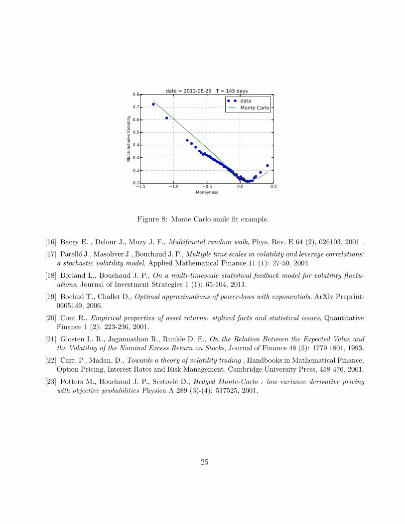
(1 + λ2)νtdWt. All equations are then discretized in the standard way, and Brownianmotions are simulated using Gaussian innovations. In order to generate the different risk factors, weuse the decomposition of Eq. (57). In figure 6 - 8 we show some example of volatility smiles. The datais composed of mid-prices of OTM calls and puts with deltas in the following range |∆| ∈ [0.001, 0.999].Note that not all fits are very good, however, a bad fit to the varswap term structure does not implynecessarily a bad fit to the overall volatility surface (see figs 9 - 12).

20

0.0 0.5 1.0 1.5 2.0 2.5


2.5

2.0

1.5

1.0

0.5

0.0Skew fit 2013-08-26

data

fitλ2 =λ3 =0

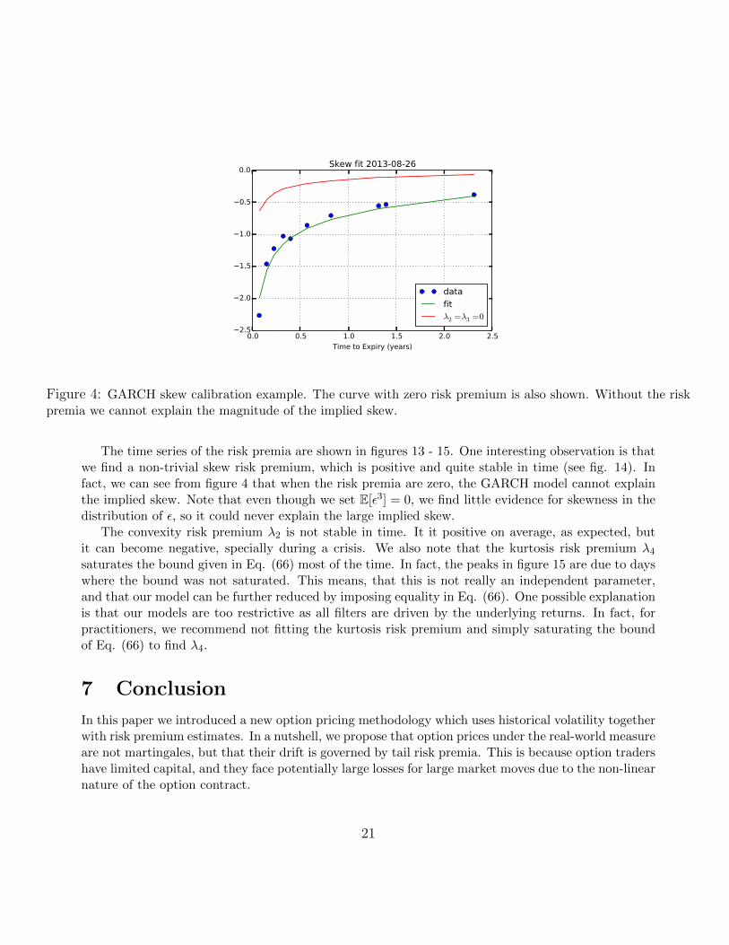
Figure 4: GARCH skew calibration example. The curve with zero risk premium is also shown. Without the riskpremia we cannot explain the magnitude of the implied skew.

The time series of the risk premia are shown in figures 13 - 15. One interesting observation is thatwe find a non-trivial skew risk premium, which is positive and quite stable in time (see fig. 14). Infact, we can see from figure 4 that when the risk premia are zero, the GARCH model cannot explainthe implied skew. Note that even though we set E[ε3] = 0, we find little evidence for skewness in thedistribution of ε, so it could never explain the large implied skew.

The convexity risk premium λ2 is not stable in time. It it positive on average, as expected, butit can become negative, specially during a crisis. We also note that the kurtosis risk premium λ4saturates the bound given in Eq. (66) most of the time. In fact, the peaks in figure 15 are due to dayswhere the bound was not saturated. This means, that this is not really an independent parameter,and that our model can be further reduced by imposing equality in Eq. (66). One possible explanationis that our models are too restrictive as all filters are driven by the underlying returns. In fact, forpractitioners, we recommend not fitting the kurtosis risk premium and simply saturating the boundof Eq. (66) to find λ4.

7 Conclusion

In this paper we introduced a new option pricing methodology which uses historical volatility togetherwith risk premium estimates. In a nutshell, we propose that option prices under the real-world measureare not martingales, but that their drift is governed by tail risk premia. This is because option tradershave limited capital, and they face potentially large losses for large market moves due to the non-linearnature of the option contract.

21

0.0 0.5 1.0 1.5 2.0 2.5


0

10

20

30

40

50

60Kurtosis fit 2013-08-26

data

fitλ2 =λ3 =λ4 =0

Figure 5: GARCH kurtosis calibration example. The curve with zero risk premium is also shown.

In particular, we have studied a general class of GARCH models with multiple time scales andasymmetry. However, we believe our procedure can be extended to any kind of volatility estimator,once we can quantify its asymptotic expansion under large movements of the underlying (e.g. tailrisks). Within the context of the models studied in this paper, we have found that, if we expandoption prices up to second order Greeks, we only need three risk premia: convexity, skew and kurtosis.However, empirically we found that the kurtosis risk premium is not independent and saturates abound, which allows us to write it in terms of the other two risk premia. Therefore, at the end, ourmodel only has two parameters that must be fitted to option prices: the convexity and skew riskpremia. The rest of the parameters are completely determined by historical data using the standardGARCH calibration methodology. This allows us to generate option smiles which are conditioned onboth our volatility forecasts and the market’s risk premia.

We found that the convexity risk premium not only shifts the level of the implied volatility but alsochanges its term structure. On the other hand, the skew risk premium makes the ATM skew steeper(more negative) than the historical estimate, and the kurtosis risk premium makes the vol-of-vol higherthan the historical one.

We developed a calibration methodology based on the vol-of-vol expansion of Bergomi and Guyon[11], where we fit a series of implied moments which can be replicated using OTM options. We thenderived approximate formulas for these moments up to second order in vol-of-vol. Once the risk premiaare found, we can generate the full volatility surface by using Monte Carlo simulations. We showedthat the smiles obtained this way are reasonably close to what is observed in the SPX option market.

There are various extensions to our work that deserve more attention. In particular, we haveassumed that we can approximate option prices to second order Greeks even though we work indiscrete time. It would be interesting to relax this assumption. Perhaps this can be done in the

22

0.4 0.3 0.2 0.1 0.0 0.1 0.2

Moneyness

0.10

0.15

0.20

0.25

0.30

0.35

0.40

0.45

Bla

ck-S

chole

s V

ola

tilit

y

date = 2013-08-26 T = 26 days

data

Monte Carlo

Figure 6: Monte Carlo smile fit example.

context of the Hedged Monte Carlo method of [23]. Another extension of our model is to make theconvexity risk premium time dependent. As we saw in section 6, the skew and kurtosis risk premiaare quite stable in time. However, this is not the case for the convexity risk premium, which can evenbecome negative during a crisis. Finally, it would be interesting to explore the relation between ourapproach and the so-called pricing kernel [7, 8].

Acknowledgments

I would like to thank Baruch University where part of this research was done. I also thank ArthurBerd, Jim Gatheral, Peter Carr, Adela Baho, Tai Ho Wang, Anja Richter, Andrew Lesniewski andFilippo Passerini for many stimulating discussions and comments on the manuscript.

References

[1] Musiela M., Rutkowski M., Martingale Methods in Financial Modeling, Springer, 2nd Edition,2005.

[2] Gatheral J., Jacquier A., Arbitrage-free SVI volatility surfaces, ArXiv preprint: 1204.0646v4, 2013.

[3] Duan J.C., The GARCH Option Pricing Model, Mathematical Finance, 5 (1): 13-32, 1995.

[4] Christoffersen P., Jacobs K., Which GARCH Model for Option Valuation, Management Science,50 (9): 1204-1221, 2004.

23

0.7 0.6 0.5 0.4 0.3 0.2 0.1 0.0 0.1 0.2

Moneyness

0.1

0.2

0.3

0.4

0.5

0.6

0.7

Bla

ck-S

chole

s V

ola

tilit

y

date = 2013-08-26 T = 54 days

data

Monte Carlo


[5] Barone-Adesi G., Engle R. F., Mancini L., A GARCH Option Pricing Model with Filtered HistoricalSimulation, Rev. Financ. Stud. 21 (3): 1223-1258, 2008.

[6] Christoffersen P., Elkamhi R., Feunou B., Jacobs K., Option Valuation with Conditional Het-eroskedasticity and Nonnormality, Rev. Financ. Stud. 23 (5): 2139-2183, 2009.

[7] Christoffersen P., Jacobs K., Heston S. , A GARCH Option Model with Variance-Dependent PricingKernel, Available at SSRN: http://ssrn.com/abstract=1538394, 2011.

[8] Babaoglu K., Christoffersen P., Heston S., Jacobs K., Option Valuation with Volatility Components,Fat Tails, and Nonlinear Pricing Kernels, Option Metrics Research Conference, New York, 2013.

[9] Taleb N. N., The Black Swan: The Impact of the Highly Improbable, Random House, 2007.

[10] Gatheral J., Oomen R.C.A., Zero-Intelligence Realized Variance Estimation, Finance Stoch. 14(2): 249-283, 2010.

[11] Bergomi L., Guyon J., The Smile in Stochastic Volatility Models, Available at SSRN:http://ssrn.com/abstract=1967470, 2011.

[12] Lo A. W., Long Term Memory in Stock Market Prices, Econometrica 59 (5): 1279-1313, 1997.

[13] Ding Z., Granger C. W. J., Engle R. F., A long memory property of stock market returns and anew model, Journal of Empirical Finance 1 (1): 83-106, 1993.

[14] Liu Y., Cizeau P., Meyer M., Peng C. K., Stanley H. E., Correlations in Economic Time Series,Physica A 245 (3)-(4): 437-440, 1997.

[15] Muzy J. F., Delour J., Bacry E., Modelling uctuations of nancial times series: from cascadeprocess to stochastic volatility model, Eur. Phys. J. B 17: 537, 2000.

24

http://ssrn.com/abstract=1538394

http://ssrn.com/abstract=1967470

1.5 1.0 0.5 0.0 0.5

Moneyness

0.1

0.2

0.3

0.4

0.5

0.6

0.7

0.8

Bla

ck-S

chole

s V

ola

tilit

y

date = 2013-08-26 T = 145 days

data

Monte Carlo


[16] Bacry E. , Delour J., Muzy J. F., Multifractal random walk, Phys. Rev. E 64 (2), 026103, 2001 .

[17] Parello J., Masoliver J., Bouchaud J. P., Multiple time scales in volatility and leverage correlations:a stochastic volatility model, Applied Mathematical Finance 11 (1): 27-50, 2004.

[18] Borland L., Bouchaud J. P., On a multi-timescale statistical feedback model for volatility fluctu-ations, Journal of Investment Strategies 1 (1): 65-104, 2011.

[19] Bochud T., Challet D., Optimal approximations of power-laws with exponentials, ArXiv Preprint:0605149, 2006.

[20] Cont R., Empirical properties of asset returns: stylized facts and statistical issues, QuantitativeFinance 1 (2): 223-236, 2001.

[21] Glosten L. R., Jagannathan R., Runkle D. E., On the Relation Between the Expected Value andthe Volatility of the Nominal Excess Return on Stocks, Journal of Finance 48 (5): 1779 1801, 1993.

[22] Carr, P., Madan, D., Towards a theory of volatility trading., Handbooks in Mathematical Finance,Option Pricing, Interest Rates and Risk Management, Cambridge University Press, 458-476, 2001.

[23] Potters M., Bouchaud J. P., Sestovic D., Hedged Monte-Carlo : low variance derivative pricingwith objective probabilities Physica A 289 (3)-(4): 517525, 2001.

25

0.0 0.5 1.0 1.5 2.0 2.5


0.24

0.26

0.28

0.30

0.32

0.34

0.36Varswap fit 2011-10-19

data

fitλ2 =0

Figure 9: A not-so-good varswap fit.

0.8 0.6 0.4 0.2 0.0 0.2 0.4

Moneyness

0.2

0.3

0.4

0.5

0.6

0.7

0.8

0.9

1.0

Bla

ck-S

chole

s V

ola

tilit

y

date = 2011-10-19 T = 31 days

data

Monte Carlo

Figure 10: Monte Carlo smile fit example when the varswap fit is not good (see figure 9).

26

1.2 1.0 0.8 0.6 0.4 0.2 0.0 0.2 0.4

Moneyness

0.0

0.2

0.4

0.6

0.8

1.0

1.2

Bla

ck-S

chole

s V

ola

tilit

y

date = 2011-10-19 T = 59 days

data

Monte Carlo


1.4 1.2 1.0 0.8 0.6 0.4 0.2 0.0 0.2 0.4

Moneyness

0.1

0.2

0.3

0.4

0.5

0.6

0.7

0.8

0.9

Bla

ck-S

chole

s V

ola

tilit

y

date = 2011-10-19 T = 150 days

data

Monte Carlo


27

20052006

20072008

20092010

20112012

20132014

Date

0.15

0.10

0.05

0.00

0.05

0.10

Convexit

y R

isk

Pre

miu

m (λ

2)

Figure 13: Convexity risk premium.

20052006

20072008

20092010

20112012

20132014

Date

1

0

1

2

3

4

5

Ske

w R

isk

Pre

miu

m (λ

3)

Figure 14: Skew risk premium.

28

20052006

20072008

20092010

20112012

20132014

Date

20

0

20

40

60

80

100

120

140

160

Kurt

osi

s R

isk

Pre

miu

m (λ

4)

from fit

from bound

Figure 15: Kurtosis risk premium. We show the time series which is obtained by the fit, and the one whichcomes from saturating the bound of Eq. (66). Notice that most of the time, both time series are the same. Werecommend to simply saturating the bound and avoiding fitting the kurtosis risk premium.

29

1402.1255

Documents