14 Solving the wave equation by Fourier method

In this lecture I will show how to solve an initial–boundary value problem for one dimensional waveequation:

utt = c2uxx, 0 < x < l, t > 0, (14.1)

with the initial conditions (recall that we need two of them, since (14.1) is a mathematical formulationof the second Newton’s law):

u(0, x) = f(x), 0 < x < l,

ut(0, x) = g(x), 0 < x < l,(14.2)

where f is the initial displacement and g is the initial velocity.I start with the homogeneous boundary conditions of type I:

u(t, 0) = 0, t > 0,

u(t, l) = 0, t > 0,(14.3)

which physically means that I am studying the oscillations of a string of length l with fixed ends.Using the same ansatz

u(t, x) = T (t)X(x)

I find thatT ′′

c2T=

X ′′

X= −λ,

and hence I have two ordinary differential equations

T ′′ + c2λT = 0 (14.4)

for T , andX ′′ + λX = 0 (14.5)

for X. Using the boundary conditions (14.3) I conclude that equation (14.5) must be supplementedwith the boundary conditions

X(0) = X(l) = 0. (14.6)

Problem (14.5)–(14.6) is a Sturm–Liouville eigenvalue problem, which we already solved several times.In particular, we know that there is an infinite series of eigenvalues

λk =k2π2

l2, l = 1, 2, . . .

and the corresponding eigenfunctions

Xk(x) = Ck sin√λkx = Bk sin

πkx

l, k = 1, 2, . . . ,

Math 483/683: Partial Differential Equations by Artem Novozhilove-mail: artem.novozhilov@ndsu.edu. Spring 2016

1

moreover all the eigenfunctions are orthogonal on [0, l]. Here Ck are some arbitrary real constants.Since I know which lambdas I can use, I now can look at the solutions to (14.4). Since all my λk > 0then I have the general solution

Tk(t) = Ak cos c√

λkt+Bk sin c√

λkt = Ak cosπckx

l+Bk sin

πckx

l,

and hence each function

uk(t, x) = Tk(t)Xk(x) =

(ak cos

πckx

l+ bk sin

πckx

l

)sin

πkx

l,

solves the wave equation (14.1) and satisfies the boundary conditions (14.3). Here ak = AkCk, bk =BkCk. Since my PDE is linear I can use the superposition principle to form my solution as

u(t, x) =

∞∑k=1

uk(t, x),

my task is to determine ak and bk. For this I will need the initial conditions. Note that using the firstinitial conditions implies

f(x) =

∞∑k=1

ak sinπkx

l,

which means that

ak =2

l

ˆ l

0f(x) sin

πkx

ldx.

To use the second boundary condition I first differentiate my series and then plug in t = 0:

g(x) =∞∑k=1

bkcπk

lsin

πkx

l,

which gives me

bk =2

πkc

ˆ l

0g(x) sin

πkx

ldx.

Hence I found a formal solution to my original problem. I am writing “formal” since I must also checkthat all the series are convergent and can be differentiated twice in t and x to guarantee that whatI found is a classical solution. Note that contrary to the heat equation, my series representations ofsolutions do not have quickly vanishing exponents and hence the question on differentiability is not assimple as before. Putting some additional smoothness requirements on the initial conditions can beused to conclude that my series are classical solutions.

Now let me see what I can infer from the found solution.The found functions uk are called the normal modes. Using the following trick:

A cosαt+B sinαt =√

A2 +B2

(A√

A2 +B2cosαt+

B√A2 +B2

sinαt

)=

√A2 +B2 (cosϕ cosαt+ sinϕ sinαt)

= R cos(αt− ϕ), ϕ = tan−1 B

A,R =

√A2 +B2,

2

I can rewrite the normal modes in the form

uk(t, x) = Rk cos

(cπkt

l− ϕk

)sin

πkx

l. (14.7)

Recall that f is periodic with period T if

f(t+ T ) = f(t)

for any t. The (minimal) period is the smallest T > 0 in this formula. Clearly if f is T -periodic then

f(t+ kT ) = f(t), k ∈ Z.

Moreover, if f is T -periodic then f(at) has period T/a (prove it). These basic facts imply that thenormal modes are periodic functions with respect to variable t with the periods

Tk =2l

ck,

because cosine is a 2π-periodic function. More importantly all normal modes have period 2l/c (notnecessarily minimal), which allows me to conclude that the solution to the problem (14.1)–(14.3) is2l/c-periodic:

T = 2l

√ρ

E.

The angular frequencies are

ωk =2π

T=

πck

l.

The normal modes are also called the harmonics. The first harmonic is the normal mode of the lowestfrequency, which is called the fundamental frequency

ω1 =πc

l.

And now I finally can make my first big conclusion here: all harmonics in the solution to the initial-boundary value problem for the wave equation are multiple of the fundamental frequency ω1, andthis is the mathematical explanation why we like the sound of musical instruments whose geometryis one-dimensional: violin, guitar, flute, etc.

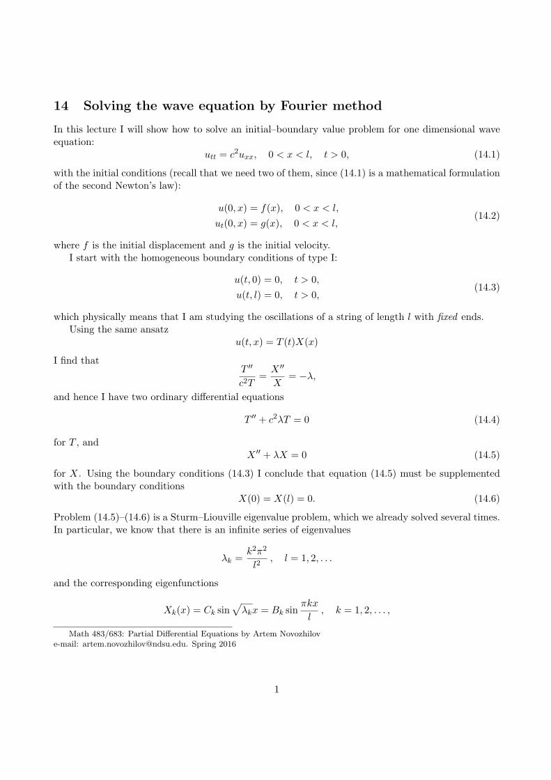
Geometrically harmonics represent standing waves (see Fig. 1) Using the introduced terminologyI can conclude that the solution to the wave equation is a sum of standing waves. However, we alsoknow that if the wave equation has no boundary conditions then the solution to the wave equation isa sum of traveling waves. This is still true (recall the reflection principle) if the boundary conditionsare imposed. So, how these two facts can be reconciled? Do we have a contradiction or these are twosides of the same phenomenon?

Actually for this particular example there is a very simple explanation:

cos(θ − ϕ) + cos(θ + ϕ) = 2 cos θ cosϕ,

and hence, any standing wave can be represented as a sum of two traveling waves.

3

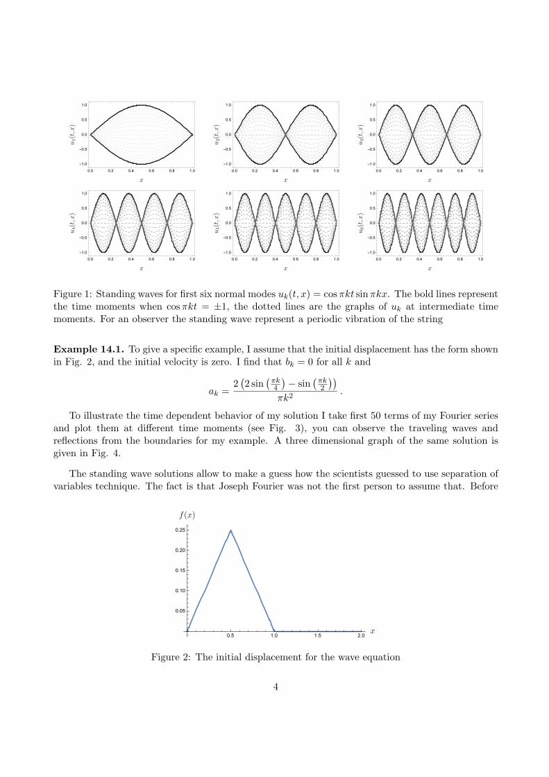
Figure 1: Standing waves for first six normal modes uk(t, x) = cosπkt sinπkx. The bold lines representthe time moments when cosπkt = ±1, the dotted lines are the graphs of uk at intermediate timemoments. For an observer the standing wave represent a periodic vibration of the string

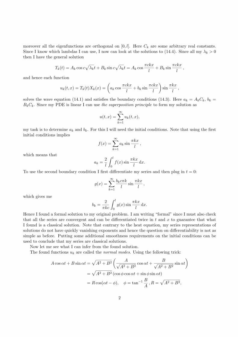
Example 14.1. To give a specific example, I assume that the initial displacement has the form shownin Fig. 2, and the initial velocity is zero. I find that bk = 0 for all k and

ak =2(2 sin

(πk4

)− sin

(πk2

))πk2

.

To illustrate the time dependent behavior of my solution I take first 50 terms of my Fourier seriesand plot them at different time moments (see Fig. 3), you can observe the traveling waves andreflections from the boundaries for my example. A three dimensional graph of the same solution isgiven in Fig. 4.

The standing wave solutions allow to make a guess how the scientists guessed to use separation ofvariables technique. The fact is that Joseph Fourier was not the first person to assume that. Before

Figure 2: The initial displacement for the wave equation

4

Figure 3: Solutions to the problem (14.1)–(14.3) with the initial displacement as in Fig. 2 and initialvelocity g(x) = 0 at different time moments. First 50 terms of the Fourier series are shown

Figure 4: Solutions to the problem (14.1)–(14.3) with the initial displacement as in Fig. 2 and initialvelocity g(x) = 0 in t, x, u(t, x) coordinates. First 50 terms of the Fourier series are shown

5

Figure 5: Two extracts from D. Bernoulli’s 1753 paper

him exactly the same guess was used by Lagrange to obtain an analytical solution to the system ofmasses on the springs (the one we used to derive in the limit the wave equation). Lagrange did nothave to deal with the questions of convergence because his “Fourier series” consisted of a finite numberof terms. Even earlier, in 1753, Daniel Bernoulli, a famous mathematician and physicist, used “Fourierseries” to represent solutions to the wave equation1. You can see his “Fourier series” in the left panelin Fig. 5. He actually did not calculate the coefficients of the series, leaving them in undeterminedform. A possible motivation for these products comes from a very careful drawing of his father, JohannBernoulli (one of the early developers of Calculus), which can be seen in Fig. 5, right panel. Theseare the drawings of the observed string oscillations, and since the graphs of standing waves look thesame and can be analytically described as a product of two trigonometric functions, one depends onlyon time and the other one only on the spatial variable, hence (we can only guess at this point) thatit was the original motivation to use the form

u(t, x) = T (t)X(x)

to solve partial differential equations.

1Bernoulli, D., 1753. Reflexions et eclaircissemens sur les nouvelles vibrations des cordes. Les Memoires de l’AcademieRoyale des Sciences et des Belles-Lettres de Berlin de 1747 et, 1748, pp.47–72.

6