14. parallel computing 14.1 introduction - harvey mudd …keller/cs60book/14 parallel...

14. Parallel Computing

14.1 Introduction

This chapter describes approaches to problems to which multiple computing agents areapplied simultaneously.

By "parallel computing", we mean using several computing agents concurrently toachieve a common result. Another term used for this meaning is "concurrency". We willuse the terms parallelism and concurrency synonymously in this book, although someauthors differentiate them.

Some of the issues to be addressed are:

What is the role of parallelism in providing clear decomposition ofproblems into sub-problems?

How is parallelism specified in computation?

How is parallelism effected in computation?

Is parallel processing worth the extra effort?

14.2 Independent Parallelism

Undoubtedly the simplest form of parallelism entails computing with totally independenttasks, i.e. there is no need for these tasks to communicate. Imagine that there is a largefield to be plowed. It takes a certain amount of time to plow the field with one tractor. Iftwo equal tractors are available, along with equally capable personnel to man them, thenthe field can be plowed in about half the time. The field can be divided in half initiallyand each tractor given half the field to plow. One tractor doesn't get into another's way ifthey are plowing disjoint halves of the field. Thus they don't need to communicate. Notehowever that there is some initial overhead that was not present with the one-tractormodel, namely the need to divide the field. This takes some measurements and might notbe that trivial. In fact, if the field is relatively small, the time to do the divisions might bemore than the time saved by the second tractor. Such overhead is one source of dilutionof the effect of parallelism.

Rather than dividing the field only two ways, if N tractors are available, it can be dividedN ways, to achieve close to an N-fold gain in speed, if overhead is ignored. However,the larger we make N, the more significant the overhead becomes (and the more tractorswe have to buy).

586 Parallel Computing

In UNIX® command-line shells, independent parallelism can be achieved by the userwithin the command line. If c1, c2, ...., cn are commands, then these commands can beexecuted in parallel in principal by the compound command:

c1 & c2 & .... & cn

This does not imply that there are n processors that do the work in a truly simultaneousfashion. It only says that logically these commands can be done in parallel. It is up to theoperating system to allocate processors to the commands. As long as the commands donot have interfering side-effects, it doesn't matter how many processors there are or inwhat order the commands are selected. If there are interfering side-effects, then theresult of the compound command is not guaranteed. This is known as indeterminacy,and will be discussed in a later section.

There is a counterpart to independent parallelism that can be expressed in C++. Thisuses the fork system call. Execution of fork() creates a new process (program inexecution) that is executing the same code as the program that created it. The newprocess is called a child, with the process executing fork being called the parent. Thechild gets a complete, but independent, copy of all the data accessible by the parentprocess.

When a child is created using fork, it comes to life as if it had just completed the call tofork itself. The only way the child can distinguish itself from its parent is by the returnvalue of fork. The child process gets a return value of 0, while the parent gets a non-zerovalue. Thus a process can tell whether it is the parent or the child by examining thereturn value of fork. As a consequence, the program can be written so as to have theparent and child do entirely different things within the same program that they share.

The value returned by fork to the parent is known as the process id (pid) of the child.This can be used by the parent to control the child in various ways. One of the uses ofthe pid, for example, is to identify that the child has terminated. The system call wait,when given the pid of the child, will wait for the child to terminate, then return. Thisprovides a mechanism for the parent to make sure that something has been done beforecontinuing. A more liberal mechanism involves giving wait an argument of 0. In thiscase, the parent waits for termination of any one of its children and returns the pid of thefirst that terminates.

Below is a simple example that demonstrates the creation of a child process using fork ina UNIX® environment. This is C++ code, rather than Java, but hopefully it is closeenough to being recognizable that the idea is conveyed.

#include <iostream.h> // for <<, cin, cout,cerr#include <sys/types.h> // for pid_t#include <unistd.h> // for fork()#include <wait.h> // for wait()

Parallel Computing 587

main(){pid_t pid, ret_pid; // pids of forked and finishing child

pid = fork(); // do it

// fork() creates a child that is a copy of the parent// fork() returns:// 0 to the child// the pid of the child to the parent

if( pid == 0 ) { // If I am here, then I am the child process. cout << "Hello from the child" << endl << endl; }else { // If I am here, then I am the parent process. cout << "Hello from the parent" << endl << endl;

ret_pid = wait(0); // wait for the child if( pid == ret_pid ) cout << "child pid matched" << endl << endl; else cout << "child pid did not match" << endl << endl; }}

The result of executing this program is:

Hello from the parent

Hello from the child

child pid matched

14.3 Scheduling

In the UNIX® example above, there could well be more processes than there areprocessors to execute those processes. In this case, the states of non-running processesare saved in a pool and executed when a processor becomes available. This happens, forexample, when a process terminates. But it also happens when a process waits for i/o.This notion of multiprocessing is one of the key ways of keeping a processor busy whenprocesses do i/o requests.

In the absence of any priority discipline, a process is taken from the pool whenever aprocessor becomes idle. To provide an analogy with the field-plowing problem, workapportionment is simplified in the following way: Instead of dividing the field into onesegment per tractor, divide it into many small parcels. When a tractor is done plowing itscurrent parcel, it finds another unplowed parcel and does that. This scheme, sometimes


called self-scheduling, has the advantage that the tractors stay busy even if some run atmuch different rates than others. The opposite of self-scheduling, where the work isdivided up in advance, will be called a priori scheduling.

14.4 Stream Parallelism

Sets of tasks that are totally independent of each other do not occur as frequently as onemight wish. More interesting are sets of tasks that need to communicate with each otherin some fashion. We already discussed command-line versions of a form ofcommunication in the chapter on high-level functional programming. There, thecompound command

c1 | c2 | .... | cn

is similar in execution to the command with | replaced by &, as discussed earlier.However, in the new case, the processes are synchronized so that the input of one waitsfor the output of another, on a character-by-character basis, as communicated throughthe standard inputs and standard outputs. This form of parallelism is called streamparallelism, suggesting data flowing through the commands in a stream-like fashion.

The following C++ program shows how pipes can be used with the C++ iostreaminterface. Here class filebuf is used to connect file buffers that are used with streams tothe system-wide filed descriptors that are produced by the call to function pipe.

#include <streambuf.h>#include <iostream.h> // for <<, cin, cout, cerr#include <stdio.h> // for fscanf, fprintf#include <sys/types.h> // for pid_t#include <unistd.h> // for fork()#include <wait.h> // for wait()

main(){int pipe_fd[2]; // pipe file descriptors:

// pipe_fd[0] is used for the read end// pipe_fd[1] is used for the write end

pid_t pid; // process id of forked child

pipe(pipe_fd); // make pipe, set file descriptors

pid = fork(); // fork a child

int chars_read;

if( pid == 0 ) { // Child process does this

// read pipe into character buffer repeatedly, until end-of-file,


// sending what was read to cout

// note: a copy of the array pipe_fd exists in both processes

close(pipe_fd[1]); // close unused write end

filebuf fb_in(pipe_fd[0]); istream in(&fb_in);

char c;

while( in.get(c) ) cout.put(c);

cout << endl; }else { close(pipe_fd[0]); // close unused read end

filebuf fb_out(pipe_fd[1]); ostream out(&fb_out);

char c;

while( cin.get(c) ) out.put(c);

close(pipe_fd[1]);

wait(0); // wait for child to finish }}

It is difficult to present a plowing analogy for stream parallelism – this would be like thefield being forced through the plow. A better analogy would be an assembly line in afactory. The partially-assembled objects move from station to station; the parallelism isamong the stations themselves.

Exercises

Which of the following familiar parallel enterprises use self-scheduling, which use apriori scheduling, and which use stream parallelism? (The answers may be locality-dependent.)

1 • check-out lanes in a supermarket

2 • teller lines in a bank

3 • gas station pumps

4 • tables in a restaurant


5 • carwash

6 •••• Develop a C++ class for pipe streams that hides the details of file descriptors, etc.

14.5 Expression Evaluation

Parallelism can be exhibited in many kinds of expression evaluations. The UNIX®command-line expressions are indeed a form of this. But how about with ordinaryarithmetic expressions, such as

(a + b) * ((c - d) / (e + f)))

Here too there is the implicit possibility of parallelism, but at a finer level of granularity.The sum a + b can be done in parallel with the expression (c - d) / (e + f). This expressionitself has implicit parallelism. Synchronization is required in the sense that the result of agiven sub-expression can't be computed before the principal components have beencomputed. Interestingly, this form of parallelism shows up if we inspect the dag (directedacyclic graph) representation of the expression. When there are two nodes with neitherhaving a path to the other, the nodes could be done concurrently in principle.

*

+

+-

/

fedc

ba

Figure 297: Parallelism in an expression tree:The left + node can be done in parallel with any

of the nodes other than the * node.The - node can be done in parallel with the right + node.

In the sense that synchronization has to be done from two different sources, this form ofparallelism is more complex than stream parallelism. However, stream parallelism hasthe element of repeated synchronization (for each character) that scalar arithmeticexpressions do not. Still, there is a class of languages in which the above expressionmight represent computation on vectors of values. These afford the use of streamparallelism in handling the vectors.

For scalar arithmetic expressions, the level of granularity is too fine to create processes –the overhead of creation would be too great compared to the gain from doing theoperations. Instead, arithmetic expressions that can be done in parallel are usually used to


exploit the "pipelining" capability present in high-performance processors. There aretypically several instructions in execution simultaneously, at different stages. A highdegree of parallelism translates into lessened constraints among these instructions,allowing more of the instruction-execution capabilities to be in use simultaneously.

Expression-based parallelism also occurs when data structures, such as lists and trees, areinvolved. One way to exploit a large degree of parallelism is through the application offunctions such as map on large lists. In mapping a function over list, we essentially arespecifying one function application for each element of the list. Each of theseapplications is independent of the other. The only synchronization needed is in the use vs.formation of the list itself: a list element can't be used before the correspondingapplication that created it is done.

Recall that the definition of map in rex is:

map(Fun, []) => [].

map(Fun, [A | X]) => [apply(Fun, A) | map(Fun, X)].

The following figure shows how concurrency results from an application of map of afunction f to a list [x1, x2, x3, ... ]. The corresponding function in rex that evaluates thosefunction applications in parallel is called pmap.

x1 x2 x3

f f f

result list

argument list

f(x1) f(x2) f(x3)

Figure 298: Parallel mapping a function over a list for independent execution.Each copy of f can be simultaneously executing.

Exercises

Which of the following programs can exploit parallelism for improved performance oversequential execution? Informally describe how.

1 •• finding the maximum element in an array


2 •• finding an element in a sorted array

3 •• merge sort

4 •• insertion sort

5 •• Quicksort

6 ••• finding a maximum in a uni-modal array (an array in which the elements areincreasing up to a point, then decreasing)

7 •• finding the inner-product of two vectors

8 •• multiplying two matrices

14.6 Data-Parallel Machines

We next turn our attention to the realization of parallelism on actual computers. There aretwo general classes of machines for this purpose: data-parallel machines and control-parallel machines. Each of these classes can be sub-divided further. Furthermore, eachclass of machines can simulate the other, although one kind of machine will usually bepreferred for a given kind of problem.

Data parallel machines can be broadly classified into the following:

SIMD multiprocessorsVector ProcessorsCellular Automata

SIMD Multiprocessors

"SIMD" stands for "single-instruction stream, multiple data stream". This means thatthere is one stream of instructions controlling the overall operation of the machine, butmultiple data operation units to carry out the instructions on distinct data. The generalstructure of a SIMD machine can thus be depicted as follows:


Control Processor

Control Program Memory

Data Processor

Data Memory

Data Processor

Data Memory

Data Processor

Data Memory

Data Processor

Data Memory

....

Figure 299: SIMD multiprocessor organization

Notice that in the SIMD organization, each data processor is coupled with its own datamemory. However, in order to get data from one memory to another, it is necessary foreach processor to have access to the memories of its neighbors, at a minimum. Withoutthis, the machine would be reduced to a collection of almost-independent computers.

Also not clear in the diagram is how branching (jumps) dependent on data values takeplace in control memory. There must be some way for the control processor to look atselected data to make a branch decision. This can be accomplished by instructions thatform some sort of aggregate (such as the maximum) from data values in each dataprocessors' registers.

SIMD Multiprocessors are also sometimes called array processors, due to their obviousapplication to problems in which an array can be distributed across the data memories.

Vector Processors

The name "vector processor" sounds similar to "array processor" discussed above.However, vector processor connotes something different to those in the field: a processorin which the data stored in registers are vectors. Typically there are both scalar registersand vector registers, with the instruction code determining whether an addressed registeris one or the other. Vector processors differ from array processors in that not all elementsof the vector are operated on concurrently. Instead pipelining is used to reduce the cost ofa machine that might otherwise have one arithmetic unit for each vector element.

Typically, vector operations are floating-point. Floating point arithmetic can be brokeninto four to eight separate stages. This means that a degree of concurrency equal to thenumber of stages can be achieved without additional arithmetic units. If still greaterconcurrency is desired, additional pipelined arithmetic units can be added, and the vectorsapportioned between them.


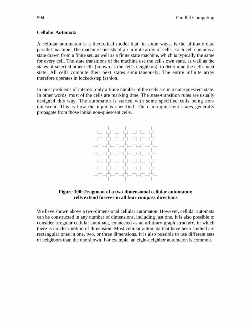
Cellular Automata

A cellular automaton is a theoretical model that, in some ways, is the ultimate dataparallel machine. The machine consists of an infinite array of cells. Each cell contains astate drawn from a finite set, as well as a finite state machine, which is typically the samefor every cell. The state transitions of the machine use the cell's own state, as well as thestates of selected other cells (known as the cell's neighbors), to determine the cell's nextstate. All cells compute their next states simultaneously. The entire infinite arraytherefore operates in locked-step fashion.

In most problems of interest, only a finite number of the cells are in a non-quiescent state.In other words, most of the cells are marking time. The state-transition rules are usuallydesigned this way. The automaton is started with some specified cells being non-quiescent. This is how the input is specified. Then non-quiescent states generallypropagate from those initial non-quiescent cells.

Figure 300: Fragment of a two-dimensional cellular automaton;cells extend forever in all four compass directions

We have shown above a two-dimensional cellular automaton. However, cellular automatacan be constructed in any number of dimensions, including just one. It is also possible toconsider irregular cellular automata, connected as an arbitrary graph structure, in whichthere is no clear notion of dimension. Most cellular automata that have been studied arerectangular ones in one, two, or three dimensions. It is also possible to use different setsof neighbors than the one shown. For example, an eight-neighbor automaton is common.


Figure 301: Four- vs. eight-neighbor cellular automata

Cellular automata were studied early by John von Neumann. He showed how Turingmachines can be embedded within them, and moreover how they can be made toreproduce themselves. A popular cellular automaton is Conway's "Game of Life". Life isa two-dimensional cellular automaton in which each cell has eight neighbors and onlytwo states (say "living" and "non-living", or simply 1 and 0). The non-living statecorresponds to the quiescent state described earlier.

The transition rules for Life are very simple: If three of a cell's neighbors are living, thecell itself becomes living. Also, if a cell is living, then if its number of living neighbors isother than two or three, it becomes non-living.

The following diagram suggests the two kinds of cases in which the cell in the center isliving in the next state. Each of these rules is only an example. A complete set of ruleswould number sixteen.

Figure 302: Examples of Life rules

Many interesting phenomena have been observed in the game of life, including patternsof living cells that appear to move or "glide" through the cellular space, as well aspatterns of cells that produce these "gliders".

Figure 303: A Life glider pattern


It has been shown that Life can simulate logic circuits (using the presence or absence of aglider to represent a 1 or 0 "flowing" on a wire). It has also been shown that Life cansimulate a Turing machine, and therefore is a universal computational model.

Exercises

1 • Enumerate all of the life rules for making the center cell living.

2 •• Write a program to simulate an approximation to Life on a bounded grid. Assumethat cells outside the grid are forever non-living.

3 •• In the Fredkin automaton, there are eight neighbors, as with life. The rules are thata cell becomes living if it is non-living and an odd number of neighbors are living.It becomes non-living if it is living and an even number of neighbors are living.Otherwise it stays as is. Construct a program that simulates a Fredkin automaton.Observe the remarkable property that any pattern in such an automaton willreproduce itself in sufficient time.

Figure 304: The Fredkin automaton, with an initial pattern


Figure 305: The Fredkin automaton, after 8 transitions from the initial pattern

4 ••• For the Fredkin automaton, make a conjecture about the reproduction time as afunction of the number of cells to be reproduced.

5 •• Show that any Turing machine can be simulated by an appropriate cellularautomaton.

6 •••• Write a program to simulate Life on an unbounded grid. This program will haveto dynamically allocate storage when cells become living that were never livingbefore.

7 ••••• A "garden-of-Eden" pattern for a cellular automaton is one that cannot be thesuccessor of any other state. Find such a pattern for Life.

14.7 Control-Parallel Machines

We saw earlier how data-parallel machines rely on multiple processors conductingsimilar operations on each of a large set of data. In control-parallel machines, there aremultiple instruction streams and no common control. Thus these machines are also oftencalled MIMD ("Multiple-Instruction, Multiple-Data") machines. Within this category,there are two predominant organizations:

Shared memory

Distributed memory


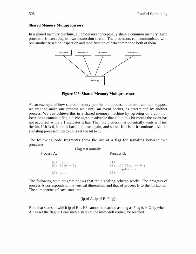
Shared Memory Multiprocessors

In a shared memory machine, all processors conceptually share a common memory. Eachprocessor is executing its own instruction stream. The processors can communicate withone another based on inspection and modification of data common to both of them.

Processor Processor Processor Processor

Memory

....

Figure 306: Shared Memory Multiprocessor

As an example of how shared memory permits one process to control another, supposewe want to make one process wait until an event occurs, as determined by anotherprocess. We can achieve this in a shared memory machine by agreeing on a commonlocation to contain a flag bit. We agree in advance that a 0 in this bit means the event hasnot occurred, while a 1 indicates it has. Then the process that potentially waits will testthe bit. If it is 0, it loops back and tests again, and so on. If it is 1, it continues. All thesignaling processor has to do is set the bit to 1.

The following code fragments show the use of a flag for signaling between twoprocesses.

Flag = 0 initiallyProcess A: Process B:

A1: .... B1: ....A2: Flag = 1; B2: if( Flag == 0 )

goto B2;A3: .... B3: ....

The following state diagram shows that the signaling scheme works. The progress ofprocess A corresponds to the vertical dimension, and that of process B to the horizontal.The components of each state are:

(ip of A, ip of B, Flag)

Note that states in which ip of B is B3 cannot be reached as long as Flag is 0. Only whenA has set the flag to 1 can such a state (at the lower-left corner) be reached.


A1, B1, 0

A2, B1, 0

A3, B1, 1

A1, B2, 0

A2, B2, 0

A3, B2, 1

A1, B3, 0

A2, B3, 0

A3, B3, 1

Figure 307: State-transition diagram of multiprocessor flag signaling

The type of signaling described above is called "busy-waiting" because the loopingprocessor is kept busy, but does no real work. To avoid this apparent waste of theprocessor as a resource, we can interleave the testing of the bit with some useful work. Orwe can have the process "go to sleep" and try again later. Going to sleep means that theprocess gives up the processor to another process, so that more use is made of theresource.

Above we have shown how a shared variable can be used to control the progress of oneprocess in relation to another. While this type of technique could be regarded as a featureof shared memory program, it can also present a liability. When two or more processorsshare memory, it is possible for the overall result of a computation to fail to be unique.This phenomenon is known as indeterminacy. Consider, for example, the case where twoprocessors are responsible for adding up a set of numbers. One way to do this would be toshare a variable used to collect the sum. Depending on how this variable is handled,indeterminacy could result. Suppose, for example, that a process assigns the sum variableto a local variable, adds a quantity to the local variable, then writes back the result to thesum:

local = sum;local += quantity to be added;sum = local;

Suppose two processes follow this protocol, and each has its own local variable. Supposethat sum is initially 0 and one process is going to add 4 and the other 5. Then dependingon how the individual instructions are interleaved, the result could be 9 or it could be 4 or5. This can be demonstrated by a state diagram. The combined programs are

A1: localA = sum; B1: localB = sum;A2: localA += 4; B2: localA += 5;A3: sum = localA; B3: sum = localB;A4: B4:


The state is:

(ip of A, ip of B, localA, localB, sum)

A1, B1, _, _, 0

A2, B1,0, _, 0

A3, B1, 4, _, 0

A1, B2, _, 0, 0

A2, B2, 0, 0, 0

A3, B2, 4, 0, 0

A1, B3, _, 5, 0

A2, B3, 0, 5, 0

A3, B3, 4, 5, 0

A1, B4, _, 5, 5

A2, B4,5, 5, 5

A3, B4, 9, 5, 5

A4, B1, 4, _, 4 A4, B2, 4, 4, 4 A4, B3, 4, 9, 4 A4, B4, 9, 9,9

A4, B2, 4, 0, 4 A4, B3, 4, 5, 4

A2, B4, 0, 5, 5

A3, B4, 4, 5, 5

A4, B4, 4, 5, 4

A4, B4, 4, 5,5

Figure 308: A state diagram exhibiting indeterminacy

Note that in the state diagram there are three states having the ip components A4, B4,each with a different value for sum. One state corresponds to the two processes havingdone their operations one after the other, and the other two corresponds to one processwriting while the other is still computing. Thus we have indeterminacy in the final valueof sum. This phenomenon is also called a race condition, as if processes A and B wereracing with each other to get access to the shared variable.

Race conditions and indeterminacy are generally undesirable because they make itdifficult to reason about parallel programs and to prove their correctness. Variousabstractions and programming techniques can be used to reduce the possibilities forindeterminacies. For example, if we use a purely functional programming model, thereare no shared variables and no procedural side-effects. Yet there can still be a substantialamount of parallelism, as seen in previous examples, such as the function map.


Semaphores

Computer scientists have worked extensively on the problem of using processorresources efficiently. They have invented various abstractions to not only allow a processto go to sleep, but also to wake it when the bit has been set, and not sooner. One suchabstraction is known as a semaphore. In one form, a semaphore is an object that containsa positive integer value. The two methods for this object are called P and V. When P isdone on the semaphore, if the integer is positive, it is lowered by one (P is from a Dutchword meaning "to lower") and the process goes on. If it is not positive, however, theprocess is put to sleep until a state is reached in which lower can be done without makingthe integer negative. The only way that such a state is reached is by another processexecuting the V ("to raise") operation. If no process is sleeping for the semaphore, the Voperation simply increments the integer value by one. If, on the other hand, at least oneprocess is sleeping, one of those processes is chosen for awakening and the integer valueremains the same (i.e. the net effect is as if the value had been raised and then lowered,the latter by the sleeping process that was not able to lower it earlier). The exact order forawakening is not specified. Most often, the process sleeping for the longest time isawakened next, i.e. a queue data structure is used.

The following program fragments show the use of a semaphore for signaling.

Semaphore S's integer value is 0 initially

Process A: Process B:

A1: .... B1: ....A2: V(S); B2: P(S)A3: .... B3: ....

The state-transition diagram is similar to the case using an integer flag. The maindifference is that no looping is shown. If the semaphore value is 0, process B simplycannot proceed. The components of each state are:

(ip of A, ip of B, Semaphore value)


A1, B1, 0

A2, B1, 0

A3, B1, 1

A1, B2, 0

A2, B2, 0

A3, B2, 1

A1, B3, 0

A2, B3, 0

A3, B3, 1

Figure 309: State diagram for signaling using a semaphore

Above we saw a flag and a semaphore being used to synchronize one process to another.Another type of control that is often needed is called mutual exclusion. In contrast tosynchronization, this form is symmetric. Imagine that there is some data to which twoprocesses have access. Either process can access the data, but only one can access it at atime. The segment of code in which a process accesses the data is called a criticalsection. A semaphore, initialized to 1 rather than 0, can be used to achieve the mutualexclusion effect.

Semaphore S's integer value is 1 initially

Process A: Process B:

A1: .... B1: ....A2: P(S); B2: P(S)A3: critical section B3: critical sectionA4: V(S) B4: V(S)A5: .... B5: ....

A useful extension of the semaphore concept is that of a message queue or mailbox. Inthis abstraction, what was a non-negative integer in the case of the semaphore is replacedby a queue of messages. In effect, the semaphore value is like the length of the queue. Aprocess can send a message to another through a common mailbox. For example, we canextend the P operation, which formerly waited for the semaphore to have a positive value,to return the next message on the queue:

P(S, M); sets M to the next message in S

If there is no message in S when this operation is attempted, the process doing P will waituntil there is a message. Likewise, we extend the V operation to deposit a message:


V(S, M); puts message M into S

Mailboxes between UNIX® processes can be simulated by an abstraction known as apipe. A pipe is accessed in the same way a file is accessed, except that the pipe is notreally a permanent file. Instead, it is just a buffer that allows bytes to be transferred fromone process to another in a disciplined way. As with an input stream, if the pipe iscurrently empty, the reading process will wait until something is in the pipe. In UNIX®,a single table common to all processes is used to hold descriptors for open files. Pipes arealso stored in this table. A pipe is created by a system call that returns two filedescriptors, one for each end of the pipe. The user of streams in C++ does not typicallysee the file descriptors. These are created dynamically and held in the state of the streamobject. By appropriate low-level coding, it is possible to make a stream object connect toa pipe instead of a file.

Exercises

1 •• Construct a state-transition diagram for the case of a semaphore used to achievemutual exclusion. Observe that no state is reached in which both processes are intheir critical sections.

2 ••• Show that a message queue can be constructed out of ordinary semaphores. (Hint:Semaphores can be used in at least two ways: for synchronization and for mutualexclusion.)

3 ••• Using a linked-list to implement a message queue, give some examples of whatcan go wrong if the access to the queue is not treated as a critical section.

14.8 Distributed Memory Multiprocessors

A distributed memory multiprocessor provides an alternative to shared memory. In thistype of design, processors don't contend for a common memory. Instead, each processoris closely linked with its own memory. Processors must communicate by sendingmessages to one another. The only means for a processor to get something from anotherprocessor's memory is for the former to send a message to the latter indicating its desire.It is up to the receiving processor to package a response as a message back to therequesting processor.


Processor Processor Processor Processor....

Memory

Communication Switch or Bus

Memory Memory Memory

Figure 310: Distributed Memory Multiprocessor

What possible advantage could a distributed memory multiprocessor have? For onething, there is no contention for a common memory module. This improves performance.On the other hand, having to go through an intermediary to get information is generallyslower than in the case of shared memory.

A related issue is known as scalability. Assuming that there is enough parallelisminherent in the application, one might wish to put a very large number of processors towork. Doing this exacerbates the problem of memory contention: only one processor canaccess a single memory module at a time. The problem can be alleviated somewhat byadding more memory modules to the shared memory configuration. The bottleneck thenshifts to the processor-memory communication mechanism. If, for example, a businterconnection is used, there is a limit to the number of memory transactions per unittime, as determined by the bus technology. If the number of processors and memorymodules greatly exceeds this limit, there will be little point in having multiple units. Toovercome the bus limitation, a large variety of multi-stage interconnect switches havebeen proposed. A typical example of such a switch is the butterfly interconnection, asshown below.

P P P P P P P P

M M M M M M M M

S S S S

S S S S

S S S S

Figure 311: Butterfly interconnection for shared memory


A major problem with such interconnection schemes is known as cache coherency. Ifprocessors cache data in memory, there is the possibility that one processor could have adatum in its cache while another processor updates the memory version of that datum. Inorder to manage this possibility, a cached copy would have to be invalidated wheneversuch an update occurs. Achieving this invalidation requires communication from thememory to the processor, or some kind of vigilance (called "snooping") in theinterconnection switch. On the other hand, a distributed memory computer does not incurthe cache coherency problem, but rather trades this for a generally longer access time forremote data.

Distributed memory multiprocessors bet on a high degree of locality, in the sense thatmost accesses will be made to local memory, in order to achieve performance. They alsomask latency of memory accesses by switching to a different thread when a remoteaccess is needed.

Networking and Client-Server Parallelism

Another type of distributed memory computer is a computer network. In this type ofsystem, several computers, each capable of operating stand-alone, are interconnected.The interconnection scheme is typically in the nature of a bus, such as an Ethernet®.These networks were not originally conceived for purposes of parallel computing asmuch as they were for information sharing. However, they can be used for parallelcomputing effectively if the degree of locality is very high.

A common paradigm for parallel computing in a network is known as client-server. Inthis model, long-term processes running on selected nodes of the network provide aservice for processes on other nodes. The latter, called clients, communicate with theserver by sending it messages. Many servers and clients can be running concurrently. Agiven node might support both client and server processes. Furthermore, a server of onefunction might be a client of others. The idea is similar to object-oriented computing,except that the objects in this case run concurrently with each other, rather than beingdormant until the next message is received.

From the programmer's point of view, communication between client and server takesplace using data abstractions such as sockets. The socket concept permits establishmentof a connection between a client and a server by the client knowing the server's address inthe network. Knowing the address allows the client to send the server an initial connectmessage. After connection is established, messages can be exchanged without the need,by the program, to use the address explicitly. Of course, the address is still used implicitlyto route the message from one node to another. A common form of socket is called thestream socket. In this form, once the connection is established, reading and writingappears to be an ordinary i/o operation, similar to using streams in C++.


14.9 Speedup and Efficiency

The speedup of a parallel computation is the ratio of the sequential execution time to theparallel execution time for the same problem. Conventions vary as to whether the samealgorithm has to be used in both time computaions. The most fair comparison is probablyto compare the speed of the parallel algorithm to that of the best-known sequentialalgorithm.

An ideal speedup factor would be equal to the number of processors, but rarely is thisachieved. The reasons that prevent it from being achieved are: (i) not all problems lendthemselves to parallel execution; some are inherently sequential, and (ii) there isoverhead involved in creating parallel tasks and communicating between them.

The idea of efficiency attempts to measure overhead; it is defined as the amount of workactually done in a parallel computation divided by the product of the run-time and thenumber of processors, the latter product being regarded as the effort

A thorough study of speedup issues is beyond the scope of this book. Suffice it to say thatdifficulty in attaining acceptable speedup on a large class of problems has been one of themain factors in the slow acceptance of parallel computation. The other factor is the extraprogramming effort typically required to achieve parallel execution. The next chaptermentions Amdahl’s law, which is one attempt at quantifying an important issue, namelythat some algorithms might be inherently sequential.

14.9 Chapter Review

Define the following terms:

cellular automatonclient-serverdistributed-memoryefficiencyexpression parallelismforkmapMIMDpipeline processingprocessschedulingshared-memorysemaphoreSIMDspeedupstream-parallelismvector processor


14.10 Further Reading

Elwyn Berlekamp, John Conway, and Richard Guy. Winning ways for your mathematicalplays, vol. 2, Academic Press, 1982. [Chapter 25 discusses the game of Life, includingself-reproduction and simulation of switching circuits. Moderate.]

A.W. Burks (ed.), Essays on cellular automata, University of Illinois Press, 1970. [Acollection of essays by Burks, von Neumann, Thatcher, Holland, and others. Includes ananalysis of von Neumann's theory of self-reproducing automata. Moderate.]

Vipin Kumar, et al., Introduction to parallel computing – Design and Analysis ofAlgorithms, Benjamin/Cummings, 1994. [Moderate.]

Michael J. Quinn, Parallel computing –theory and practice, McGraw-Hill, 1994. [Anintroduction, with emphasis on algorithms. Moderate.]

William Poundstone, The recursive universe, Contemporary books, Inc., Chicago, Ill.,1985. [A popular discussion of the game of Life and physics. Easy.]

Evan Tick, Parallel logic programming, MIT Press, 1991. [Ties together parallelism andlogic programming. Moderate.]

Stephen Wolfram, Cellular automata and complexity, Addison-Wesley, 1994. [Acollection of papers by Wolfram. Difficult.]

14. parallel computing 14.1 introduction - harvey mudd …keller/cs60book/14 parallel...

Documents