www.tesseral-geo.com

Example of Ground SurfaceModeling

-Invisible-Free-

Sep-13

“Surface” group buttons:

• “Invisible” box when checked allows to model seismic field in a way where surface is not reflecting.

• “Free” produces a “true” free surface, where the real surface conditions are modeled.

• “Static” option allows simulating reflections from the model surface, which will have the same phase as theincoming waves (as in case of velocity/density skipping to higher values). If source is placed near the surface its initialimpulse will be altered by positive reflection from the model surface. “Static” option does not work for “Scalar” equation type(§1.2 ).

No reflected from surfacewave

Reflected from surface wave has the same phase(reflection from boundary with significantly lower seismic

impedance)

Reflected from surface wave changes phase on opposite(reflection from boundary with significantly higher seismic

impedance)

basics

Static Surface, Acoustic

Free Surface, Acoustic

Static Surface, Elastic

Static Surface, Acoustic

How “StaticSurface” works?

basics

FreeSurface

Advanced

4

ModelVD

Source 5 m deepReceivers 2.4 m deep

Following modeling results are referenced to this model. If source and receivers are on the model surface, for computations, they are

automatically “deepened” inside the medium at the computational grid 4 cell sizes(here, 0.6 m*4=2.4 m).

Vx Vz

Elastic wave equation, PF- (peak frequency) attenuation (Q) used

5

advanced

ModelOD

Source 5 m deepReceivers 2.4 m deep

Vx Vz

Elastic wave equation, PF- (peak frequency) attenuation (Q) used

6

advanced

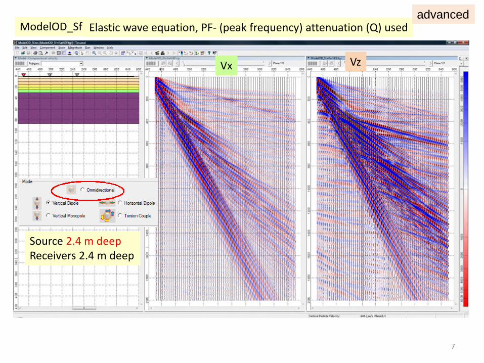
ModelOD_Sf

Source 2.4 m deepReceivers 2.4 m deep

Vx Vz

Elastic wave equation, PF- (peak frequency) attenuation (Q) used

7

advanced

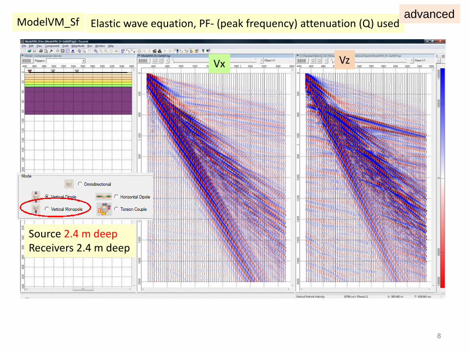
ModelVM_Sf

Source 2.4 m deepReceivers 2.4 m deep

Vx Vz

Elastic wave equation, PF- (peak frequency) attenuation (Q) used

8

advanced

ModelVD ModelOD

ModelOD_Sf ModelVM_Sf

Source 5 m deep

Source 2.4 m deep

Modeling results show identical times for same events, but they have different relativemagnitude depending on source mode and depth. For example, surface waves vs others, P-waves vs S-waves, Vz vs Vx, etc.

Q-factor used

9

Air

10

advanced

ModelVD_Air

Comparison of modeling with upper Air half-space.Using of Q-factor considerably attenuates “day surface ringing” skin-effect.

Vz

Q used:Air Q=20, Surface Layer Q=40

No Q

Air

11

advanced

ModelVD_Air

Comparison of modeling with upper Air half-space.Smaller value of Q-factor in upper layer (loose soil) is even more decreasing “daysurface ringing” skin-effect.

Vz

Q used:Air Q=20, Surface Layer Q=40

Q used:Air Q=20, Surface Layer Q=20

Air

12

advanced

13

Definitions of Stoneley wave on the Web:• A surface wave (interface wave) associated with the

interface between two solid media. The wave is ofmaximum intensity at the interface and decreasesexponentially away from the interface into bothsolids.

en.wikipedia.org/wiki/Stoneley_wave

Relating to Lamb-Stoneley - ... accociated with theinterface between solid and liquid media. Airformally also may be related to liquid (acoustic)media, with only difference that gas is considerablyless dense (and consequently more compressible).

Sharp surface and Lamb-Stoneley waves

Well is presented horizontally, source at coordinate X=0 inside of the well filled with claydrilling mud (acoustic medium).

Borehole environment represents homogeneous medium (elastic) complicated with horizontal(with this orientation – vertical) higher velocity layer.

Receivers are positioned at the side of hole from 3 m to 7 m with interval 0.152 m.Source pick frequency 10 000 Hz.The computation grid cell size 0.01 m.Recording sampling 0.000 000 5 sec.

Model of well sonic logging

Well

Borehole environment

sourcereceivers

compressionalvelocity color scale

Z, m

X, m

2D-2C modeling case

14

Left picture represents modeled shotgather; right picture – seismic wave field snapshot (at starting)Red line on shotgather – current time of the snapshot

Blue arrow – compressional wave propagating along side of the boreholeGreen arrow – converted shear PS-wave;Red arrow –Stoneley wave, forming train, which is characteristic for surface waves

15

Left picture – snapshot at time 0.0012 secBlue arrows - compressional waves: 1- direct wave from the source, 2- head (conical) wave,3- direct wave propagating in borehole environment;Green arrows – converted PS-waves: 4- direct wave propagating in borehole environment, 5-head (conical) wave;Red arrows – Stoneley waves, sharply attenuating outside of boundary. Intensiveness of thosewaves is considerably higher than of compressional and converted waves, velocity is smaller thanone of shear wave, characteristic feature - forming continuous train.

12

3

45

16

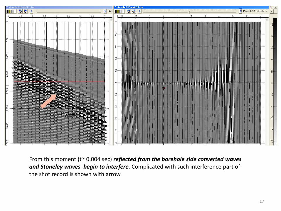
From this moment (t~ 0.004 sec) reflected from the borehole side converted wavesand Stoneley waves begin to interfere. Complicated with such interference part ofthe shot record is shown with arrow.

17

a ba- snapshot in case of one boundary (upper) over source (shown with red arrow) point ; b- snapshotin case of two boundaries (analogue of well filled with clay drilling mud (acoustic medium) in whichwas generated wave.More exactly in this (2D) modeling it is not a cylindrical well but thin infinite hollow.With blue arrow is shown first arrival of compressional wave propagating in liquid.With brown arrow – tube wave, velocity of which is considerably smaller than of compressional wave.With green arrow are shown waves relating to discontinuity.

18

Model of well sonic logging “with casing”

“Casing” Vp ~ 5000 m/s

“First Arrivals”Time field

Shotgather Snapshot

19