1.4 equilibrium of airplane 1.5 number of equations of ... 1... · 1.4 equilibrium of airplane 1.5...
TRANSCRIPT
Flight dynamics-I Prof. E.G. Tulapurkara
Chapter-1
Dept. of Aerospace Engg., Indian Institute of Technology, Madras 1
Chapter 1
Lecture 2 Introduction – 2 Topics
1.4 Equilibrium of airplane
1.5 Number of equations of motion for airplane in flight
1.5.1 Degrees of freedom
1.5.2 Degrees of freedom for a rigid airplane
1.6 Subdivisions of flight dynamics
1.6.1 Performance analysis
1.6.2 Stability and control analysis
1.7 Additional definitions
1.7.1 Attitude of the airplane
1.7.2 Flight path
1.7.3 Angle of attack and side slip
Flight dynamics-I Prof. E.G. Tulapurkara
Chapter-1
Dept. of Aerospace Engg., Indian Institute of Technology, Madras 2
1.4 Equilibrium of airplane
The above three types of forces (aerodynamic, propulsive and
gravitational) and the moments due to them govern the motion of an airplane in
flight.
If the sums of all these forces and moments are zero, then the airplane is
said to be in equilibrium and will move along a straight line with constant velocity
(see Newton's first law). If any of the forces is unbalanced, then the airplane will
have a linear acceleration in the direction of the unbalanced force. If any of the
moments is unbalanced, then the airplane will have an angular acceleration
about the axis of the unbalanced moment.
The relationship between the unbalanced forces and the linear
accelerations and those between unbalanced moments and angular
accelerations are provided by Newton’s second law of motion. These
relationships are called equations of motion.
1.5 Number of equations of motion for an airplane in flight
To derive the equations of motion, the acceleration of a particle on the
body needs to be known. The acceleration is the rate of change of velocity and
the velocity is the rate of change of position vector with respect to the chosen
frame of reference.
1.5.1 Degrees of freedom
The minimum number of coordinates required to prescribe the motion is
called the number of degrees of freedom. The number of equations governing
the motion equals the degrees of freedom. As an example, it may be recalled
that the motion of a particle moving in a plane is prescribed by the x- and y-
coordinates of the particle at various instants of time and this motion is described
by two equations.
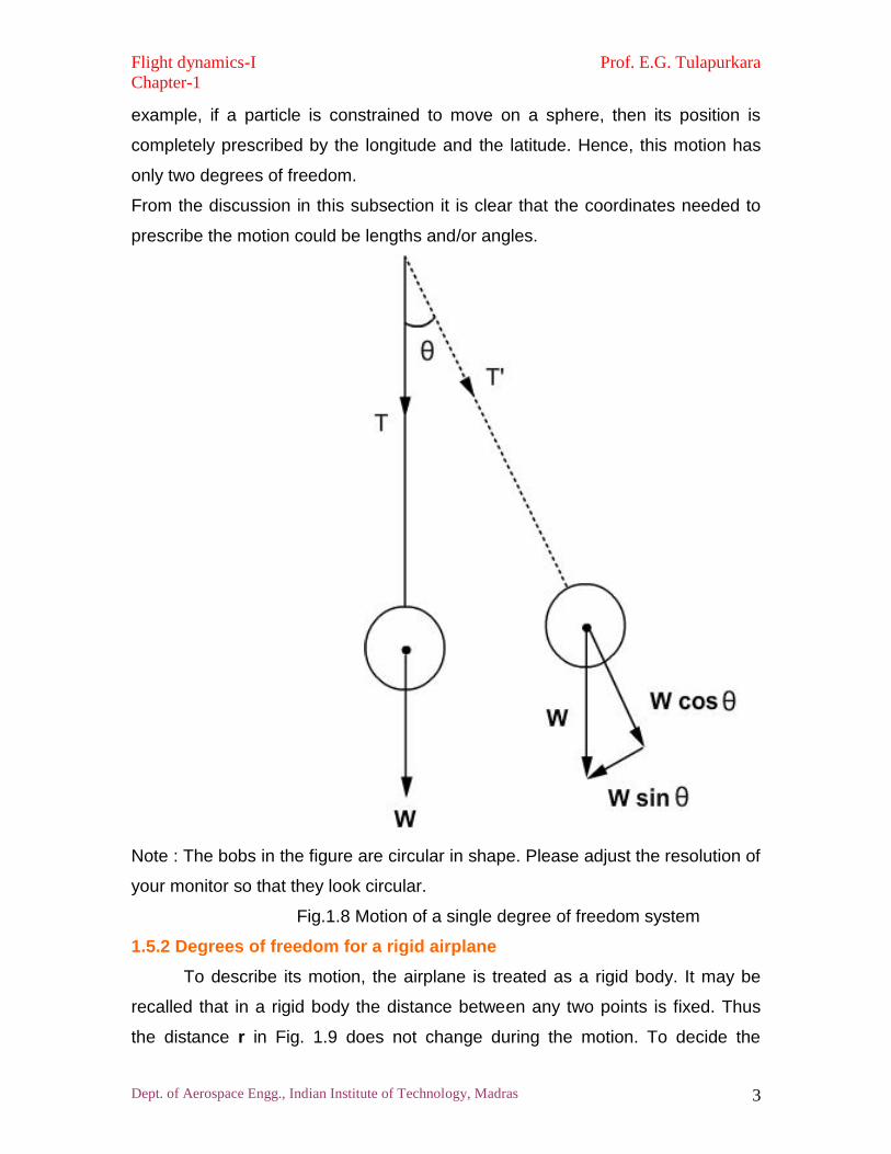
Similarly, the position of any point on a rigid pendulum is describe by just
one coordinate namely the angular position (θ) of the pendulum (Fig.1.8). In this
case only one equation is sufficient to describe the motion. In yet another
Flight dynamics-I Prof. E.G. Tulapurkara
Chapter-1
Dept. of Aerospace Engg., Indian Institute of Technology, Madras 3
example, if a particle is constrained to move on a sphere, then its position is
completely prescribed by the longitude and the latitude. Hence, this motion has
only two degrees of freedom.
From the discussion in this subsection it is clear that the coordinates needed to
prescribe the motion could be lengths and/or angles.
Note : The bobs in the figure are circular in shape. Please adjust the resolution of
your monitor so that they look circular.
Fig.1.8 Motion of a single degree of freedom system
1.5.2 Degrees of freedom for a rigid airplane
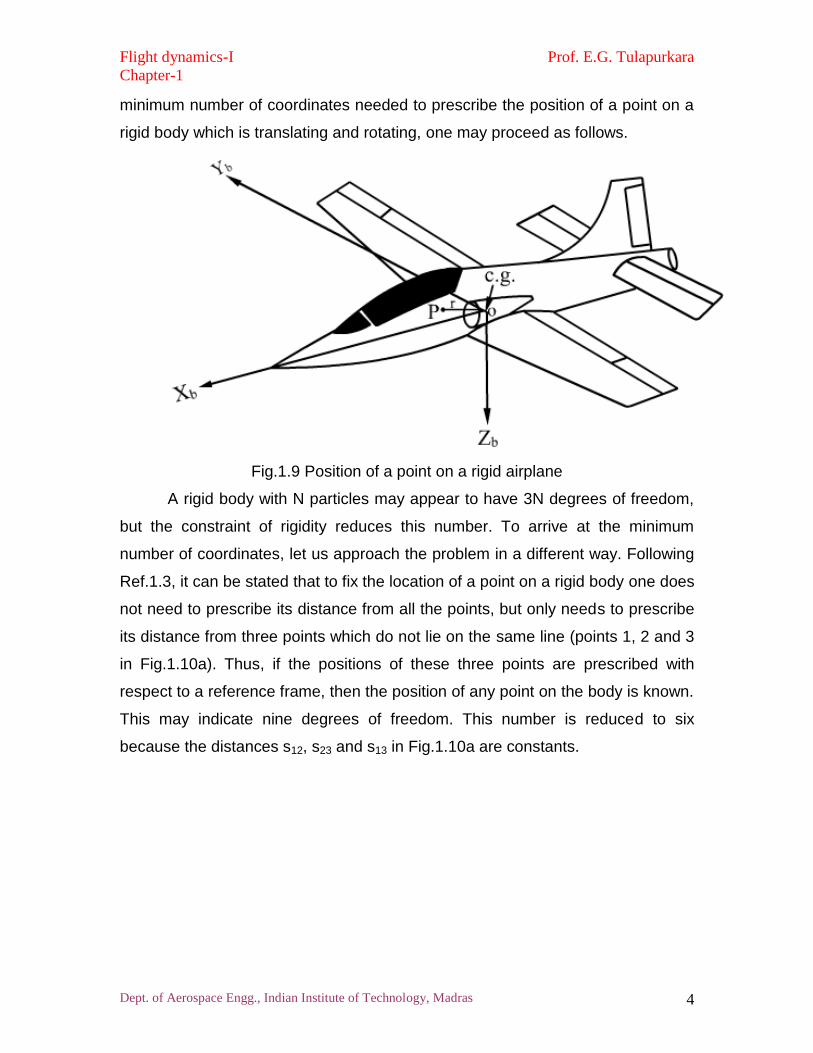
To describe its motion, the airplane is treated as a rigid body. It may be
recalled that in a rigid body the distance between any two points is fixed. Thus
the distance r in Fig. 1.9 does not change during the motion. To decide the
Flight dynamics-I Prof. E.G. Tulapurkara
Chapter-1
Dept. of Aerospace Engg., Indian Institute of Technology, Madras 4
minimum number of coordinates needed to prescribe the position of a point on a
rigid body which is translating and rotating, one may proceed as follows.
Fig.1.9 Position of a point on a rigid airplane
A rigid body with N particles may appear to have 3N degrees of freedom,
but the constraint of rigidity reduces this number. To arrive at the minimum
number of coordinates, let us approach the problem in a different way. Following
Ref.1.3, it can be stated that to fix the location of a point on a rigid body one does
not need to prescribe its distance from all the points, but only needs to prescribe
its distance from three points which do not lie on the same line (points 1, 2 and 3
in Fig.1.10a). Thus, if the positions of these three points are prescribed with
respect to a reference frame, then the position of any point on the body is known.
This may indicate nine degrees of freedom. This number is reduced to six
because the distances s12, s23 and s13 in Fig.1.10a are constants.
Flight dynamics-I Prof. E.G. Tulapurkara
Chapter-1
Dept. of Aerospace Engg., Indian Institute of Technology, Madras 5
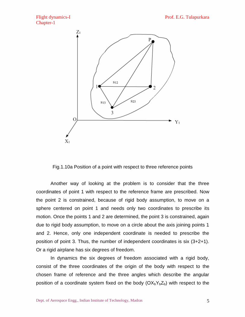
Fig.1.10a Position of a point with respect to three reference points
Another way of looking at the problem is to consider that the three
coordinates of point 1 with respect to the reference frame are prescribed. Now
the point 2 is constrained, because of rigid body assumption, to move on a
sphere centered on point 1 and needs only two coordinates to prescribe its
motion. Once the points 1 and 2 are determined, the point 3 is constrained, again
due to rigid body assumption, to move on a circle about the axis joining points 1
and 2. Hence, only one independent coordinate is needed to prescribe the
position of point 3. Thus, the number of independent coordinates is six (3+2+1).
Or a rigid airplane has six degrees of freedom.
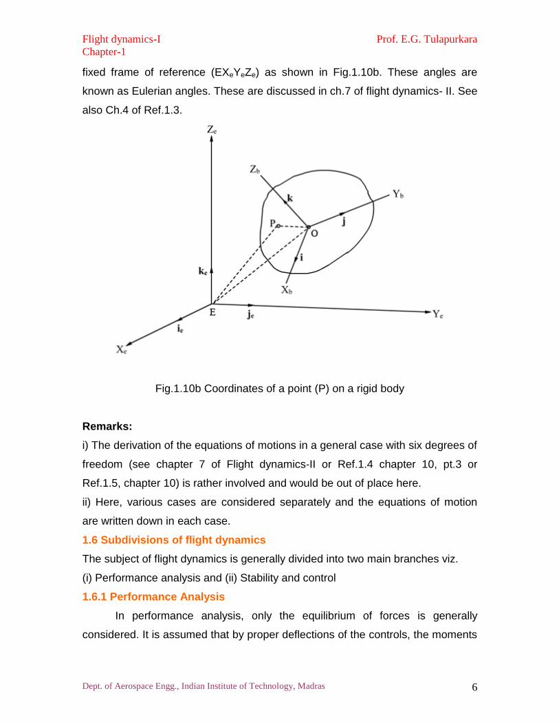
In dynamics the six degrees of freedom associated with a rigid body,
consist of the three coordinates of the origin of the body with respect to the
chosen frame of reference and the three angles which describe the angular
position of a coordinate system fixed on the body (OXbYbZb) with respect to the
Flight dynamics-I Prof. E.G. Tulapurkara
Chapter-1
Dept. of Aerospace Engg., Indian Institute of Technology, Madras 6
fixed frame of reference (EXeYeZe) as shown in Fig.1.10b. These angles are
known as Eulerian angles. These are discussed in ch.7 of flight dynamics- II. See
also Ch.4 of Ref.1.3.
Fig.1.10b Coordinates of a point (P) on a rigid body
Remarks:
i) The derivation of the equations of motions in a general case with six degrees of
freedom (see chapter 7 of Flight dynamics-II or Ref.1.4 chapter 10, pt.3 or
Ref.1.5, chapter 10) is rather involved and would be out of place here.
ii) Here, various cases are considered separately and the equations of motion
are written down in each case.
1.6 Subdivisions of flight dynamics
The subject of flight dynamics is generally divided into two main branches viz.
(i) Performance analysis and (ii) Stability and control
1.6.1 Performance Analysis
In performance analysis, only the equilibrium of forces is generally
considered. It is assumed that by proper deflections of the controls, the moments
Flight dynamics-I Prof. E.G. Tulapurkara
Chapter-1
Dept. of Aerospace Engg., Indian Institute of Technology, Madras 7
can be made zero and that the changes in aerodynamic forces due to deflection
of controls are small. The motions considered in performance analysis are steady
and accelerations, when involved, do not change rapidly with time.
The following motions are considered in performance analysis
- Unaccelerated flights,
• Steady level flight
• Climb, glide and descent
- Accelerated flights,
• Accelerated level flight and climb
• Loop, turn, and other motions along curved paths which are
called manoeuvres
• Take-off and landing.
1.6.2 Stability and control analyses
Roughly speaking, the stability analysis is concerned with the motion of
the airplane, from the equilibrium position, following a disturbance. Stability
analysis tells us whether an airplane, after being disturbed, will return to its
original flight path or not.
Control analysis deals with the forces that the deflection of the controls
must produce to bring to zero the three moments (rolling, pitching and yawing)
and achieve a desired flight condition. It also deals with design of control
surfaces and the forces on control wheel/stick /pedals. Stability and control are
linked together and are generally studied under a common heading.
Flight dynamics - I deals with performance analysis. By carrying out this
analysis one can obtain various performance characteristics such as maximum
level speed, minimum level speed, rate of climb, angle of climb, distance covered
with a given amount of fuel called ‘Range’, time elapsed during flight called
‘Endurance’, minimum radius of turn, maximum rate of turn, take-off distance,
landing distance etc. The effect of flight conditions namely the weight, altitude
and flight velocity of the airplane can also be examined. This study would also
help in solving design problems of deciding the power required, thrust required,
Flight dynamics-I Prof. E.G. Tulapurkara
Chapter-1
Dept. of Aerospace Engg., Indian Institute of Technology, Madras 8
fuel required etc. for given design specifications like maximum speed, maximum
rate of climb, range, endurance etc.
Remark:
Alternatively, the performance analysis can be considered as the analysis
of the motion of flight vehicle considered as a point mass, moving under the
influence of applied forces (aerodynamic, propulsive and gravitational forces).
The stability analysis similarly can be considered as motion of a vehicle of finite
size, under the influence of applied forces and moments.
1.7 Additional definitions
1.7.1 Attitude
As mentioned in section 1.5.2 the instantaneous position of the airplane,
with respect to the earth fixed axes system (EXeYeZe), is given by the
coordinates of the c.g. at that instant of time. The attitude of the airplane is
described by the angular orientation of the OXbY
bZ
b system with respect to
OXeYeZe system or the Euler angles. Reference 1.4, chapter 10 may be referred
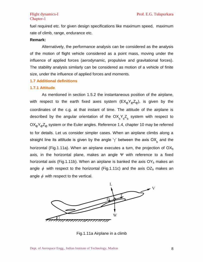
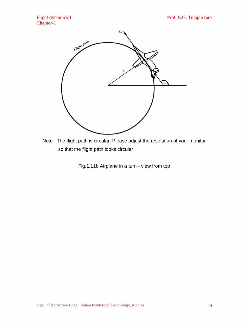
to for details. Let us consider simpler cases. When an airplane climbs along a
straight line its attitude is given by the angle ‘γ’ between the axis OXb and the
horizontal (Fig.1.11a). When an airplane executes a turn, the projection of OXb
axis, in the horizontal plane, makes an angle Ψ with reference to a fixed
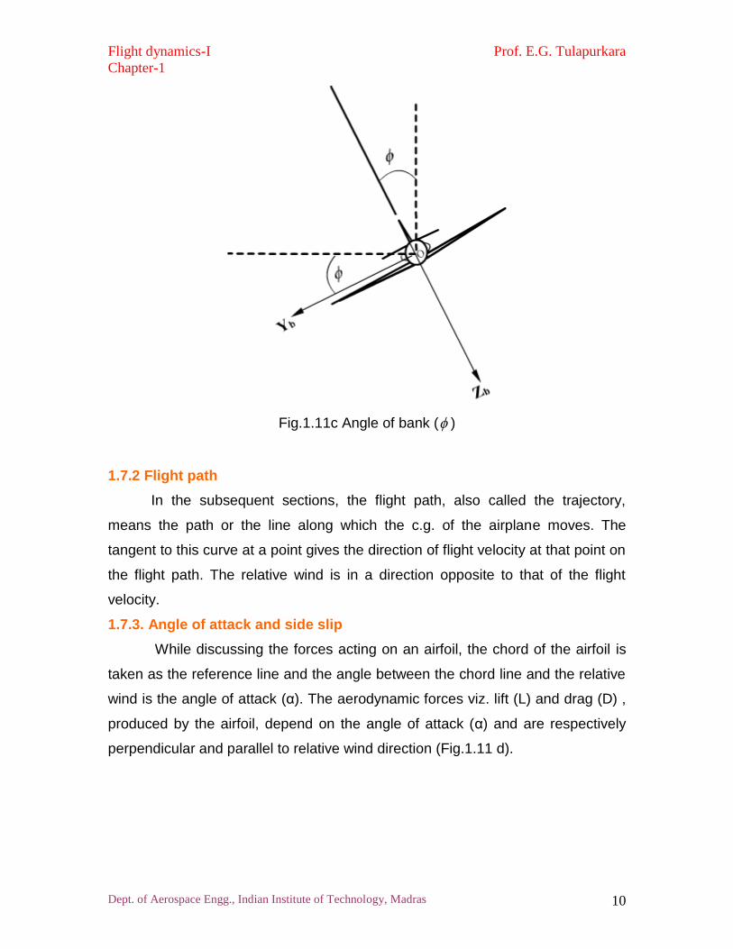
horizontal axis (Fig.1.11b). When an airplane is banked the axis OYb makes an
angle with respect to the horizontal (Fig.1.11c) and the axis OZb makes an
angle with respect to the vertical.
Fig.1.11a Airplane in a climb
Flight dynamics-I Prof. E.G. Tulapurkara
Chapter-1
Dept. of Aerospace Engg., Indian Institute of Technology, Madras 9
Note : The flight path is circular. Please adjust the resolution of your monitor
so that the flight path looks circular
Fig.1.11b Airplane in a turn - view from top
Flight dynamics-I Prof. E.G. Tulapurkara
Chapter-1
Dept. of Aerospace Engg., Indian Institute of Technology, Madras 10
Fig.1.11c Angle of bank ( )
1.7.2 Flight path
In the subsequent sections, the flight path, also called the trajectory,
means the path or the line along which the c.g. of the airplane moves. The
tangent to this curve at a point gives the direction of flight velocity at that point on
the flight path. The relative wind is in a direction opposite to that of the flight
velocity.
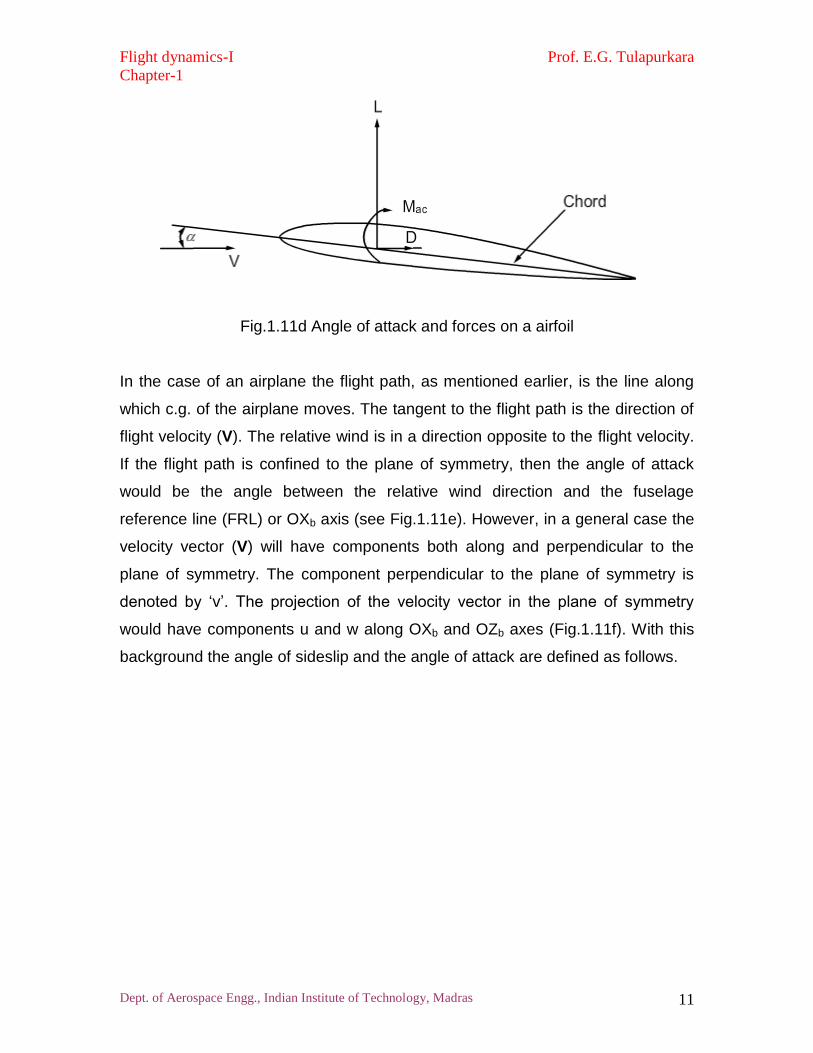
1.7.3. Angle of attack and side slip
While discussing the forces acting on an airfoil, the chord of the airfoil is
taken as the reference line and the angle between the chord line and the relative
wind is the angle of attack (α). The aerodynamic forces viz. lift (L) and drag (D) ,
produced by the airfoil, depend on the angle of attack (α) and are respectively
perpendicular and parallel to relative wind direction (Fig.1.11 d).
Flight dynamics-I Prof. E.G. Tulapurkara
Chapter-1
Dept. of Aerospace Engg., Indian Institute of Technology, Madras 11
Fig.1.11d Angle of attack and forces on a airfoil
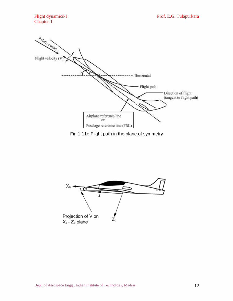
In the case of an airplane the flight path, as mentioned earlier, is the line along
which c.g. of the airplane moves. The tangent to the flight path is the direction of
flight velocity (V). The relative wind is in a direction opposite to the flight velocity.
If the flight path is confined to the plane of symmetry, then the angle of attack
would be the angle between the relative wind direction and the fuselage
reference line (FRL) or OXb axis (see Fig.1.11e). However, in a general case the
velocity vector (V) will have components both along and perpendicular to the
plane of symmetry. The component perpendicular to the plane of symmetry is
denoted by ‘v’. The projection of the velocity vector in the plane of symmetry
would have components u and w along OXb and OZb axes (Fig.1.11f). With this
background the angle of sideslip and the angle of attack are defined as follows.
Flight dynamics-I Prof. E.G. Tulapurkara
Chapter-1
Dept. of Aerospace Engg., Indian Institute of Technology, Madras 12
Fig.1.11e Flight path in the plane of symmetry
Flight dynamics-I Prof. E.G. Tulapurkara
Chapter-1
Dept. of Aerospace Engg., Indian Institute of Technology, Madras 13
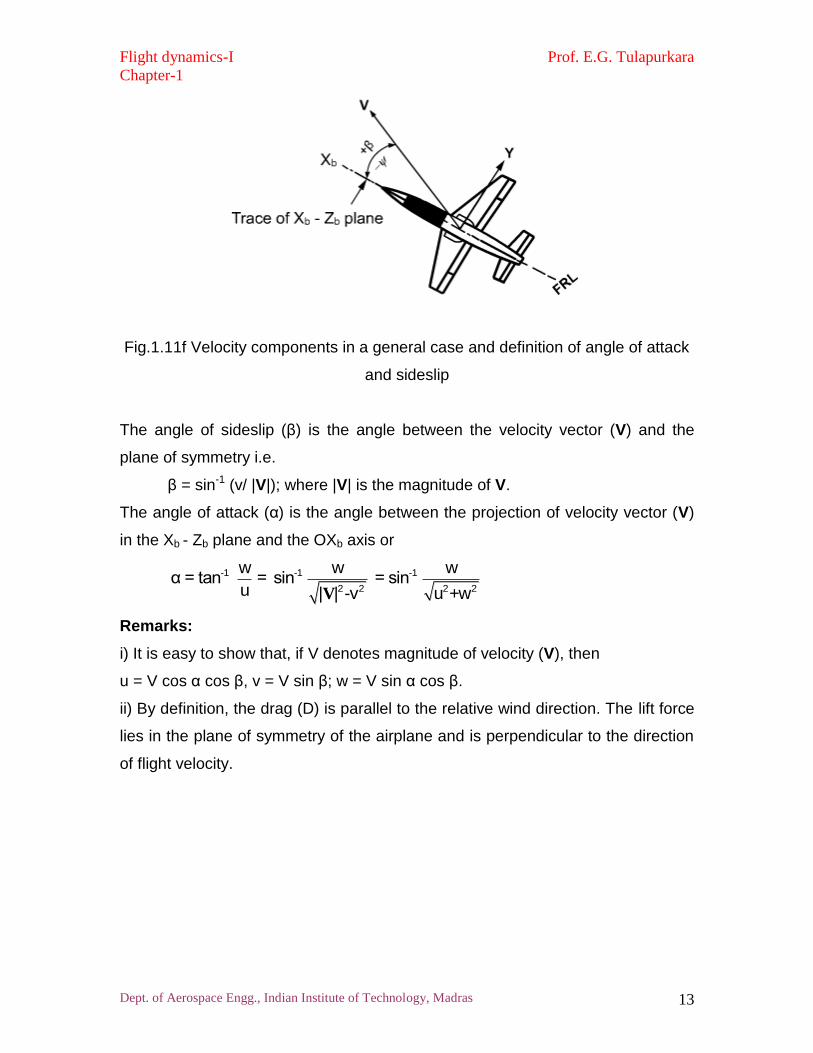
Fig.1.11f Velocity components in a general case and definition of angle of attack
and sideslip
The angle of sideslip (β) is the angle between the velocity vector (V) and the
plane of symmetry i.e.
β = sin-1 (v/ |V|); where |V| is the magnitude of V.
The angle of attack (α) is the angle between the projection of velocity vector (V)
in the Xb - Zb plane and the OXb axis or
-1 -1 -1
2 2 2 2
w w wα = tan = sin = sin
u | | -v u +wV
Remarks:
i) It is easy to show that, if V denotes magnitude of velocity (V), then
u = V cos α cos β, v = V sin β; w = V sin α cos β.
ii) By definition, the drag (D) is parallel to the relative wind direction. The lift force
lies in the plane of symmetry of the airplane and is perpendicular to the direction
of flight velocity.