14 Cost Minimization

Optional Reading: Varian, Chapters 20, 21.1-21.3 & 22.1-22.7.

In principle, everything we want to know about competitive �rms can be derived from

pro�t maximization problem. One can derive:

� Factor demands

� Firm supply

Adding over all �rms in the economy we get market factor demands and supply of goods

and combining with the demand for goods and supply of factors, which come from either

exogenous resource constraints (land) or adding over demands and supplies from standard

consumer problems (or if a \factor" is an intermediate good from other pro�t maximization

problems) we get a full blown equilibrium model.

However, as we saw in the example, the pro�t maximization problem is rather com-

plex and sometimes ill-de�ned and it turns out that it is useful to separate the problem to

maximize pro�ts into two steps:

Step 1 For a given level of output y; �nd the cheapest way to produce any given level of

output.

Step 2 Select the best level of output.

The advantages of this approach are that

1. Tractability: It is easier to think about the relevant trade-o�s when we break up

problem in parts.

2. The �rst step, the cost minimization problem, is the same regardless of whether the

market (for the output good) is competitive, the �rm is a monopolist or if there is some

intermediate situation with \imperfect" competition. This facilitates comparisons of

di�erent market forms.

137

14.1 The Cost Minimization Problem

We ask, which is the cheapest way to produce a given level of output for a �rm that takes

factor prices as given and has access to some technology summarized by the production

function f (x1; x2) : That is

minx1;x2

w1x1 + w2x2

s.t. f(x1; x2) = y:

Now, you may think that this is something di�erent from what we have done before due to

the \min" operator replacing the \max". However:

� If (x�1; x�2) is a solution to the minimization problem that means that w1x

�1 + w2x

�2 �

w1x1 + w2x2 for all (x1; x2) that satis�es f(x1; x2) = y:

� But w1x�1 + w2x

�2 � w1x1 + w2x2 , � (w1x

�1 + w2x

�2) � � (w1x1 + w2x2)

� ) � (w1x�1 + w2x

�2) � � (w1x1 + w2x2) for all (x1; x2) that satis�es f(x1; x2) = y:

Which means that (x�1; x�2) solves

maxx1;x2

�w1x1 � w2x2

s.t. f(x1; x2) = y:

Now, in principle the constraint can be solved for x2 as a function of x1 and you can then

plug this into the objective function and dervve a solution by taking �rst order conditions

in the exact same way as when we solved utility maximization problems. Alternatively,

Lagrangian methods can be applied (if you know how you are welcome to use Lagrangians

when solving constrained optimization problems. For this particular problem it is actually

more convenient due to the potentially non-linear constraint). Since I want to keep the math

at a very basic level I will make sure that all problems you will see can be solved without

Lagrangians (that is, f (x1; x2) will have simple enough form so that you can solve it out).

We will return later to the (less important) problem how to calculate solutions. Here,

the more important thing is to see conceptually how cost minimization relates to pro�t

138

maximization. Write

x1 (w1; w2; y)

x2 (w1; w2; y)

For the solution to the cost minimization problem (which you can derive in exactly the

same way as the solution to the utility maximization problem in consumer theory). In

analogue with the utility maximization problem the solution will depend on the parameters

(the exogenous variables) of the problem. That is, exactly as price and income changes will

change the best consumer bundle in consumer theory, factor price changes and how much

you are supposed to produce will change the factor inputs that produces the target output

in the cheapest possible way. Now, we can de�ne

C (w1; w2; y) = w1x1 (w1; w2; y) + w2x2 (w1; w2; y) =

=minx1;x2 w1x1 + w2x2

s.t f(x1; x2) = y

This function C (w1; w2; y) is called the minimal cost function or simply the cost function.

Now the problem to maximize pro�ts is

maxx1;x2;y

py � w1x1 � w2x2

subj to y � f (x1; x2)

Let y� be a pro�t maximizing output level (together with some factor inputs of course). We

note that the optimal factor inputs must solve

maxx1;x2

py� � w1x1 � w2x2

subj to y� � f (x1; x2) ;

where py� is just a constant. This problem is equivalent (see discussion on max versus min

above) with the cost minimization problem.

The important consequence of this is that this means that if we have a given cost function

we can look for the pro�t maximizing output level by solving the problem

maxy

py � C (w1; w2; y) :

139

This is a simple enough univariate calculus problem and sometimes referred to as the �rm

supply problem ( i.e., in Varian chapter 22)

14.2 Solving the Cost Minimization Problem

We will again proceed both graphically and by actually solving the problem using calculus.

Here these approaches complements each other to a larger extent than previously. The

picture gives a clear intuition, but the relationship with pro�t maximization is not seen as

easily. The calculus approach is less intuitive, but here the way cost minimization is used as

an intermediate step to solve the pro�t maximization problem is easier to see.

14.2.1 Graphical Treatment

6

bbbbbbbbbbbbbbb

bbbbbbbbb

bbbbbbbbbbbbbbbbbbb -

�����3

Highercosts

slope �w1

w2

C

w1

C

w2

x2

x1

Figure 1: Lines with Constant Costs

The idea is to proceed as we did when \solving" the pro�t maximization problem with a

picture in Section ??. Consider all combinations of factor inputs that corresponds to some

given cost level C; that is

C = w1x1 + w2x2 ,

x2 =C

w2�w1

w2x1;

140

which de�nes a family of straight lines called \isocosts" in Varian. The cost minimization

problem is to produce a given output at the lowest possible cost, so in terms of a graph it

is then clear that if we put in the level curve of f (x1; x2) that shows the combinations of

inputs that gives this level of output y (i.e., the isoquant corresponding to y) the solution

to the cost minimization problem occurs at the line that touches the given isoquant which

is closest to the origin of the graph. Once again it is then apparent that the solution must

occur where there is a tangency between the isoquant and the isocost since otherwise it is

possible to move towards lower cost levels and still produce the same output.

6

bbbbbbbbbbbbbbb -

�����3

Highercosts

C

w1

C

w2

x2

x1

s

y = f(x1; x2)

x�

1

x�

2

bbbbbbbbbbbbbbbb

Figure 2: The Cost Minimization Problem

In our discussion of technology we showed that the slope of the level curve is given by

�

@f(x1;x2)@x1

@f(x1;x2)@x2

� TRS (x1; x2) ;

so the optimum condition is@f(x�1;x�2)

@x1

@f(x�1;x�2)@x2

=w1

w2

This makes perfect sense:

� The technical rate of substitution tells you how much extra factor 2 needed if output

is to be kept constant and factor 1 reduced by a small unit.

\The rate at which �rms can substitute factors"

141

� The relative factor price w1w2

gives the \rate at which factors can be exchanged in the

market".

14.3 Some Examples

14.3.1 Fixed Proportions

C (w1; w2; y) = minx1;x2

w1x1 + w2x2

s.t y = min fx1; x2g

)

x1 (w1; w2; y) = y

x2 (w1; w2; y) = y

)

C (w1; w2; y) = (w1 + w2) y

14.3.2 Cobb Douglas

C (w1; w2; y) = minx1;x2

w1x1 + w2x2

s.t y = xa1xb2

Solving the constraint we get

x2 = y1bx�a

b1

Plugging into the objective we get

C (w1; w2; y) = minx1

w1x1 + w2y1bx�a

b1

Or, you may write this as

maxx1�w1x1 � w2y

1bx�a

b1

142

The �rst order condition is

�w1 � w2y1b

��a

b

�x�a

b�1

1 = 0

or

w1 = w2y1ba

bx�(a+bb )1 , multiply with x

a+bb

1

w1xa+bb

1 = w2y1ba

bx�(a+bb )1 x

a+bb

1 = w2y1ba

b

or

xa+bb

1 =w2

w1

a

by1b ,

x1 (w1; w2; y) =�w2

w1

a

b

� ba+b

y1

a+b

Symmetrically we get (either by observing the symmetry or by plugging back in constraint)

that

x2 (w1; w2; y) =

w1

w2

b

a

! aa+b

y1

a+b

and plugging this into the objective we get the cost function

C (w1; w2; y) = w1

�aw1

bw2

� ba+b

y1

a+b + w2

bw2

aw1

! aa+b

y1

a+b ;

which looks really ugly. However, competitive analysis assumes that prices and factor prices

are exogenous for the �rm. Hence, from the perspective of analyzing the supply problem

for the �rm the really important property of the cost function is to say how costs change

with output. This exercise is for �xed factor prices and we note that we then may write the

resulting cost function for a Cobb Douglas technology as

C (y) = Ky1

a+b ;

where

K = w1

�aw1

bw2

� ba+b

+ w2

bw2

aw1

! aa+b

We then see that

C 0 (y) = K1

a+ by

1a+b

�1

is:

143

1. Increasing in y if a + b < 1: That is, the marginal cost is increasing when there is

decreasing returns to scale.

2. Decreasing in y if a + b > 1: That is, the marginal cost is decreasing with increasing

returns to scale.

3. Constant in y if a+ b = y: That is the marginal cost is constant with constant returns

to scale.

14.3.3 A Remark about Notation

Once again, note that:

� w1; w2; y are parameters of the cost minimization problem

� x1; x2 are the choice variables.

The solution to the cost minimization problem will then in general give the choice vari-

ables as functions of the parameters. We write these as

x1 (w1; w2; y)

x2 (w1; w2; y)

and call them conditional factor demands. Now, plugging in these in the objective we get

the cost function

C (w1; w2; y) = w1x1 (w1; w2; y) + w2x2 (w1; w2; y) :

One of the more confusing aspects of economics is that sometimes we write something as a

function of a long list of parameters and sometimes we write the same thing as a function

of a shorter list, maybe just a single parameter. This practice simply re ects that for some

purposes we want to keep a bunch of parameters constant and for other purposes we want to

see what happens when we change these parameters. For that reason, the list of parameters

that is explicitly introduced in the notation depends on the question we want to ask.

144

The cost function is a perfect example. If we want to study factor substitution we keep

w1; w2 in the notation and study how factor shares are a�ected when the relative factor price

changes. However, often times we will not experiment with changes in factor prices and then

we write

x1 (y)

x2 (y)

for the conditional factor demands and

C (y) = w1x1 (y) + w2x2 (y)

For the cost function. This is purely a matter of convenience and for any particular tech-

nology there is a particular cost function and the formula for this function typically involves

w1 and w2: However, this is now implicitly incorporated in \the functional relation".

15 Average, Marginal and Total Costs

We will now take the cost function derived in the section on cost minimization as given and

introduce some terminology that is useful in order to think about �rm supply decisions. Since

we are not going to chine factor prices we are lazy and write C(y) rather than C (w1; w2; y) ;

but it is conceptually important that you keep in mind we are still studying exactly the same

creature. Now:

� C(y)y

is called the average cost

� dC(y)dy

is called the marginal cost.

Often we think about cost functions that have a �xed cost component (costs for setting

up a plant or R&D etc.) and write

C (y) = Cv (y) + F;

where Cv (y) is the variable cost function and F is the �xed cost. We than call

145

� Cv(y)y

the average variable cost

� Fythe average �xed cost

There are lots of relations between these curves and you can read about this in Varian.

However, a few facts are important for understanding of graphs:

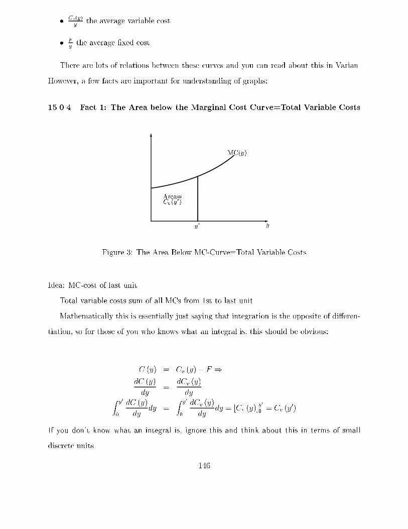
15.0.4 Fact 1: The Area below the Marginal Cost Curve=Total Variable Costs

6

-y

MC(y)

y0

Area=Cv(y

0)

Figure 3: The Area Below MC-Curve=Total Variable Costs

Idea: MC-cost of last unit

Total variable costs-sum of all MCs from 1st to last unit

Mathematically this is essentially just saying that integration is the opposite of di�eren-

tiation, so for those of you who knows what an integral is, this should be obvious:

C (y) = Cv (y) + F )

dC (y)

dy=

dCv (y)

dyZ y0

0

dC (y)

dydy =

Z y0

0

dCv (y)

dydy = [Cv (y)]

y0

0 = Cv (y0)

If you don't know what an integral is, ignore this and think about this in terms of small

discrete units.

146

15.0.5 Fact 2: MC and AVC curve starts at same place

6

-y

MC(y)

AVC(y)

Figure 4: MC and AVC Curves Starts at same Place

Idea: Average variable cost of �rst small unit and marginal cost for the �rst small unit is

the same thing. I.e., Marginal cost at zero is

dC (0)

dy=dCv (0)

dy= lim

y!0

Cv (y)� Cv (0)

y= lim

y!0

Cv (y)

y

and Cv(y)y

is just the average cost.

15.0.6 Fact 3: AVC decreasing whenever MC curve is below AVC curve and

AVC increasing whenever MC curve is above AVC curve.

Idea: The way to decrease an average is to add numbers that are below the average

Math:

d

dy

Cv (y)

y=

dCv(y)dy

y � Cv (y)

y2=

=

dCv(y)dy

� Cv(y)y

y=MC (y)� AV C (y)

y

147

6

-y

MC(y)AVC(y)

Figure 5: MC Decreasing i� AVC>MC

16 Supply of a Competitive Firm

Optional Reading: Varian, Chapter 22.

A competitive �rm take the price of the product(s) it sells as given, so the pro�t maxi-

mizing level of output is the solution to

maxy

py � C(y)

Observe here the analytical advantage of using the cost function rather than to write down

the \complete" problem

maxx1;x2

pf(x1; x2)� w1x1 � w2x2:

The cost function C(y) includes all relevant information about the production function

f (x1; x2) and factor prices and as you will see this means that we can graphically depict the

�rm supply function in pictures that should be familiar from Econ 101. Now, the �rst order

condition to the \�rm supply" problem is

p� C 0(y) = 0, p = C 0(y):

148

Which simply says that �rms should produce output up to the point where the marginal cost

of production is equal to the price. This should be highly intuitive since if the last produced

unit would cost more than the price to produce, then the �rm would be better o� reducing

output. If on the other hand, the last produced unit would cost less to produce than the

price the �rm gets on the market, then pro�ts would increase if output is increased.

16.1 How to Handle Multiple Solutions to p =MC

It is important to understand what the condition p =MC is. It is a necessary condition for

an interior solution. Hence there are two things to worry about. First of all it may be that

there are several output levels consistent with the condition. Second of all, the solution may

be a boundary solution (that is producing nothing).

6

-y

MC(y) AVC(y)

p0

y00y0

Figure 6: Solution can't be where MC curve slope downwards

In many circumstances it is reasonable to think that the marginal cost curve is U-shaped

and this case is also the favorite case for undergraduate economics textbooks. Then, it may

very well be that there are two levels of output y that satis�es p = C 0(y) as in Figure 6.

Here the basic insight is that whatever the solution to the pro�t maximization

problem is, it must be at the upwards sloping part of the marginal cost curve.

Hence, in the case depicted in Figure 6 we see that y0 and y00 both are output levels such

149

that price equals marginal costs. However, y00 generates a higher pro�t than y0; so if either

y0 or y00 indeed is the solution, then it must be y00:

That y00 generates a higher pro�t can be understood from the picture directly. We

established above that the total variable costs equals the area below the marginal cost curve.

Hence the di�erence in variable costs between y00 and y0 is the area below the MC curve

in between y0 and y00: The di�erence in revenues is the rectangle with base given by the line

between y0 and y00 and height p: Hence, the extra pro�t from increasing production from y0

to y00 is the area in between the horizontal line at p0 and the marginal cost curve, meaning

that producing at y00 gives a higher pro�t than producing at y0:

Another way to understand the same thing is that the pro�ts can be written as

�(y) = py � C(y) = py � Cv(y)� F

= y (p� AV C(y))� F

Hence, conditional on p < AV C(y00) (see discussion below on this) it follows that:

� If y00 > y0 and

� AV C(y00) < AV C(y0); then

� �(y00) > �(y0)

Now, if you look at the picture you should see that the marginal cost curve is below p

for all y in between y0 and y00: Hence the marginal cost for each unit in between y0 and y00 is

lower than the marginal cost for the units in between 0 and y0: Hence, the average

variable cost must be lower at y00 than the cost at y0:

Note from this discussion that if the marginal cost curve is always decreasing, then there

CAN NOT be an interior solution to the supply problem. You should draw a graph and

convince yourself that this is so and why!

150

6

-y

MC(y) AVC(y)

p0

Figure 7: y = 0 Solves Problem if Price too Low

16.2 The Possibility of a Boundary Solution

In general we know that the �rst order condition is necessary only for interior solutions.

However, if

p < AV C(y)

for all choices of y; then the best thing the �rm can do is to produce nothing. Such a situation

is depicted in Figure 7. It should be clear from the picture that

�(y) = y (p� AV C(y))� F < �F = � (0)

for any y > 0: The conclusion is that:

� If the candidate solution on the upwards sloping part of the marginal cost curve occurs

where the marginal cost curve is below the average variable cost curve, then this is

indeed the solution to the pro�t maximization problem.

� However, if not, then the solution is to set y = 0:

151

16.3 The (Inverse) Supply Curve

Combining the \shutdown condition" with the fact that if the shutdown condition is satis�ed

we can depict the supply curve of the �rm as in Figure 8. Again, you should note that

conceptually we think of supply as a function of the price, i.e., the problem

maxy�0

py � C(y)

has price as an exogenous parameter. Hence, it gives an optimal solution for each p (if

problem well-de�ned as we will assume). However, for the graphs it is more convenient to

put p on the vertical axis since that corresponds to the natural way to draw the cost curves.

6

-y

MC(y) AVC(y)

p, MCAVC

Figure 8: The Firm Supply Curve

16.4 Pro�ts and Producer Surplus

In the case when there is a �xed cost, we do have to include that in the calculation of the

pro�t for the �rm. In terms of the graph this means that we have to use the average cost

curve rather than the average variable cost curve. Note that the larger is output, the closer

is the average cost curve to the average variable cost curve, which simply re ects that Fyis

decreasing in y with limy!1Fy= 0.

152

6

-y

MC(y) AVC(y)AC(y)

y�

p�

AC(y�)

Figure 9: Firm Pro�t Given price p�

In Varian and other textbooks it is common to call the pro�t net of the �xed cost F

the producer surplus. The reason for this name (I think) is that diagrammatically it is the

analogue of the consumer surplus in utility theory (don't panic-I haven't even mentioned

that in the class, but you may recall this name from Econ 101).

Now, the distinction between pro�ts and producer surplus is kind of trivial and unim-

portant when solving problems using calculus. Whether one maximizes

py � C(y) = py � Cv(y)� F

or

py � Cv(y)

doesn't matter at all since the problems only di�er by a constant. However, for drawing

pictures it is actually good not to have the �xed cost included. The reason is that we can

measure total variable costs as either the rectangle with base y� and height AV C(y�) or as

the area between the marginal cost curve and the horizontal axis (Fact 1 in our discussion of

cost curves). Hence, we can measure the producer surplus in any of the two ways depicted

in Figure 10.

153

6

y

MC(y) AVC(y)

p0

p

y�

-

6

y

MC(y) AVC(y)

p0

p

y�

-

Figure 10: Two Equivalent Ways to Measure Producer Surplus

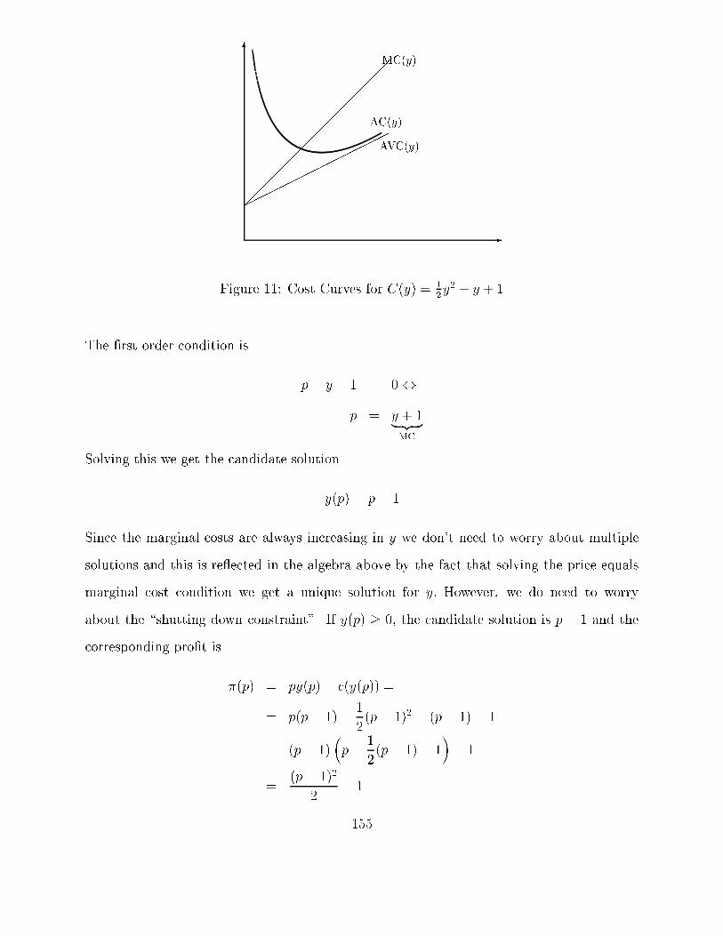
16.5 Example

Let the cost curve (i.e., the minimized cost function from some problem of cost minimization)

be given by

C(y) =1

2y2 + y + 1

and we have that:

� AC(y) = C(y)y

=12y2+y+1

y= 1

2y + 1 + 1

y

� AV C(y) = CV (y)y

=12y2+y

y= 1

2y + 1

� AFC(y) = C(0)y

= 1y

� MC(y) = C 0(y) = y + 1

We can easily solve the �rm supply problem explicitly in this example. The problem is

maxy�0

py � C(y)

or, with the particular cost function

maxy�0

py �1

2y2 � y � 1

154

6

-

�������������

����

������

���

MC(y)

AC(y)

AVC(y)

Figure 11: Cost Curves for C(y) = 12y2 + y + 1

The �rst order condition is

p� y � 1 = 0,

p = y + 1| {z }MC

Solving this we get the candidate solution

y(p) = p� 1

Since the marginal costs are always increasing in y we don't need to worry about multiple

solutions and this is re ected in the algebra above by the fact that solving the price equals

marginal cost condition we get a unique solution for y: However, we do need to worry

about the \shutting down constraint". If y(p) � 0; the candidate solution is p� 1 and the

corresponding pro�t is

�(p) = py(p)� c(y(p)) =

= p(p� 1)�1

2(p� 1)2 � (p� 1)� 1

= (p� 1)�p�

1

2(p� 1)� 1

�� 1

=(p� 1)2

2� 1

155

to be compared with

�(0) = �1

Under the assumption that p� 1 > 0 we have that �(p) = (p�1)2

2� 1 > �1 = �(0); so in this

case the solution to the interior �rst order condition is indeed the solution to the problem.

Now, if p < 1; the �rst order condition p = y + 1 isn't satis�ed for any y � 0: Intuitively it

is rather clear that in this case y (p) = 0 is the optimal solution since the marginal cost for

the �rst unit is 1 and the revenue for the �rst unit is p < 1: To see this formally, note that

if p < 1 the pro�t satis�es

py �1

2y2 � y � 1 < �

1

2y2 � 1 = �

1

2y2 � � (0) < � (0)

for all y > 0: Hence, the supply curve is

y(p) =

8><>:

0 for p < 1

p� 1 for p � 1

and the inverse supply curve can be plotted as in Figure 12

6

-))

�������������

�������������

MC(y)

AC(y)

AVC(y)

Figure 12: Firm Supply Given Cost Function for C(y) = 12y2 + y + 1

156

16.6 Supply with Constant Returns to Scale

An important special case is when there are constant returns to scale. We saw in two

examples (�xed proportions and Cobb-Douglas with a + b = 1) that this leads to a cost

function of the form

C(y) = Ky

and this is true in general for constant returns technologies. Now:

� AC(y) = AV C(y) = Ky

y= K

� MC(y) = C 0(y) = K

So the �rm supply is

y(p) =

8>>>>><>>>>>:

0 if p < K

anything if p = K

not de�ned if p > K

That is, the supply curve is at the vertical axis for prices below K and then a horizontal

line.

You may look back at what we said about why maximized pro�ts must be zero in equi-

librium with constant returns to scale. The bottom line here is that the equilibrium price

can be determined from the cost side only (which includes stu� from the technology and

factor prices).

16.7 Remark on a Figure in Varian

You may be confused when you read section 22.2 and look at Figure 22.1 in Varian. The

discussion is actually sort of OK, but it may not be clear to you what the issue is and what

the fuzz is about. The Figure and the section is meant to explain why the assumption of

a price taking �rm makes some sense. To do this Varian loosely describes a \game"

where �rms actually sets prices. We will look at this particular game towards the end of

the course, but the point here is that if �rms set prices and customers are free to choose

157

whatever �rm they want (and know what prices are posted everywhere), they'll buy at the

lowest price. If you don't get it now, ignore it and go back to the section after we've discussed

\Bertrand Competition".

158