1/30
DESCRIPTION
Cosine theta can generally be negative. So, can vector space similarity be negative?. 1/30. Project part A discussion Relevance feedback; correlation analysis; LSI. So many ways things can go wrong…. Reasons that ideal effectiveness hard to achieve: - PowerPoint PPT PresentationTRANSCRIPT

19 de abr de 2023 1
1/30
Project part A discussion
Relevance feedback; correlation analysis; LSI
Cosine theta can generally be negative. So, can vector space similarity be negative?

19 de abr de 2023 2
So many ways things can go wrong…
Reasons that ideal effectiveness hard to achieve:
1. Document representation loses information.
2. Users’ inability to describe queries precisely.
3. Similarity function used not be good enough.
4. Importance/weight of a term in representing a document and query may be inaccurate
5. Same term may have multiple meanings and different terms may have similar meanings.
Query expansionRelevance feedback
LSICo-occurrence
analysis

Improving Vector Space Ranking
• We will consider three techniques– Relevance feedback—which tries to improve the query
quality– Correlation analysis, which looks at correlations between
keywords (and thus effectively computes a thesaurus based on the word occurrence in the documents) to do query elaboration
– Principal Components Analysis (also called Latent Semantic Indexing) which subsumes correlation analysis and does dimensionality reduction.

19 de abr de 2023 7
Relevance Feedback for Vector Model
Crdj
CrNCrdj
CroptdjdjQ 11
Cr = Set of documents that are truly relevant to QN = Total number of documents
In the “ideal” case where we know the relevant Documents a priori

19 de abr de 2023 8
Rocchio Method
Dndj
DnDrdj
Dr djdjQQ ||||01
Qo is initial query. Q1 is the query after one iterationDr are the set of relevant docsDn are the set of irrelevant docs Alpha =1; Beta=.75, Gamma=.25 typically.
Other variations possible, but performance similar

19 de abr de 2023 9
Rocchio/Vector Illustration
Retrieval
Information
0.5
1.0
0 0.5 1.0
D1
D2
Q0
Q’
Q”
Q0 = retrieval of information = (0.7,0.3)D1 = information science = (0.2,0.8)D2 = retrieval systems = (0.9,0.1)
Q’ = ½*Q0+ ½ * D1 = (0.45,0.55)Q” = ½*Q0+ ½ * D2 = (0.80,0.20)

19 de abr de 2023 10
Example Rocchio Calculation
)04.1,033.0,488.0,022.0,527.0,01.0,002.0,000875.0,011.0(
12
25.0
75.0
1
)950,.00.0,450,.00.0,500,.00.0,00.0,00.0,00.0(
)00.0,020,.00.0,025,.005,.00.0,020,.010,.030(.
)120,.100,.100,.025,.050,.002,.020,.009,.020(.
)120,.00.0,00.0,050,.025,.025,.00.0,00.0,030(.
121
1
2
1
new
new
Q
SRRQQ
Q
S
R
R
Relevantdocs
Non-rel doc
Original Query
Constants
Rocchio Calculation
Resulting feedback query

19 de abr de 2023 11
Rocchio Method
Rocchio automatically re-weights terms adds in new terms (from relevant docs)
have to be careful when using negative terms
Rocchio is not a machine learning algorithm Most methods perform similarly
results heavily dependent on test collection Machine learning methods are proving to
work better than standard IR approaches like Rocchio

19 de abr de 2023 12
Rocchio is just one approach for relevance feedback… Relevance feedback—in the most general terms
—involves learning. Given a set of known relevant and known
irrelevant documents, learn relevance metric so as to predict whether a new doc is relevant or not Essentially a classification problem!
• Can use any classification learning technique (e.g. naïve bayes, neural nets, support vector m/c etc.)
Viewed this way, Rocchio is just a simple classification method
• That summarizes positive examples by the positive centroid, negative examples by the negative centroid, and assumes the most compact description of the relevance metric is vector difference between the two centroids.

Correlation/Co-occurrence analysis
Co-occurrence analysis:• Terms that are related to terms in the original query may be
added to the query.
• Two terms are related if they have high co-occurrence in documents.
Let n be the number of documents;
n1 and n2 be # documents containing terms t1 and t2,
m be the # documents having both t1 and t2
If t1 and t2 are independent
If t1 and t2 are correlated
mn
n
n
nn 21
mn
n
n
nn 21
Mea
sure
degree
of corre
lation
>> if Inversely correlated

a b c d e f g h IInterface 0 0 1 0 0 0 0 0 0User 0 1 1 0 1 0 0 0 0System 2 1 1 0 0 0 0 0 0Human 1 0 0 1 0 0 0 0 0Computer 0 1 0 1 0 0 0 0 0Response 0 1 0 0 1 0 0 0 0Time 0 1 0 0 1 0 0 0 0EPS 1 0 1 0 0 0 0 0 0Survey 0 1 0 0 0 0 0 0 1Trees 0 0 0 0 0 1 1 1 0Graph 0 0 0 0 0 0 1 1 1Minors 0 0 0 0 0 0 0 1 1
Terms and Docs as mutually dependent vectors in
Document vector
Term vector
If terms are independent, theT-T similarity matrix would be diagonal =If it is not diagonal, we can use the correlations to add related terms to the query =But can also ask the question “Are there independent dimensions which define the space where terms & docs are vectors ?”
In addition to doc-doc similarity, We can compute term-term distance

Association Clusters• Let Mij be the term-document matrix
– For the full corpus (Global)
– For the docs in the set of initial results (local)
– (also sometimes, stems are used instead of terms)
• Correlation matrix C = MMT (term-doc Xdoc-term =
term-term)
djtvdjtudj
ffCuv ,,
CuvCvvCuuCuvSuv
CuvSuv
Un-normalized Association Matrix
Normalized Association Matrix
Nth-Association Cluster for a term tu is the set of terms tv such that Suv are the n largest values among Su1, Su2,….Suk

Example
d1d2d3d4d5d6d7
K1 2 1 0 2 1 1 0
K2 0 0 1 0 2 2 5
K3 1 0 3 0 4 0 0
11 4 6
4 34 11
6 11 26
1.0 0.097 0.193
0.097 1.0 0.224
0.193 0.224 1.0
Correlatio
n
Matrix
Norm
alized
Correlation
Matrix
1th Assoc Cluster for K2 is K3
4)12(34)22(11)11(4)12(
12 ssssS
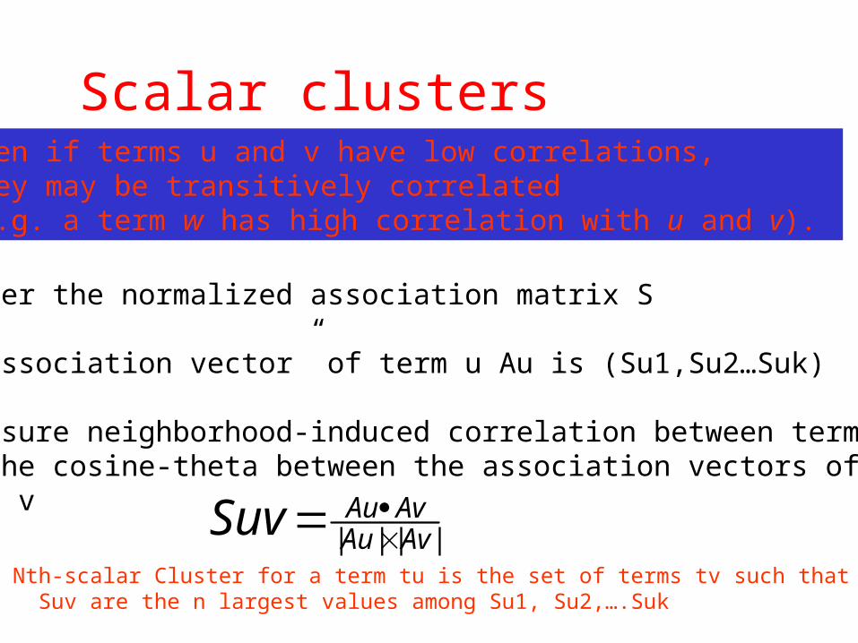
Scalar clusters
Consider the normalized association matrix S
The “association vector” of term u Au is (Su1,Su2…Suk)
To measure neighborhood-induced correlation between terms:Take the cosine-theta between the association vectors of terms u and v
Even if terms u and v have low correlations, they may be transitively correlated (e.g. a term w has high correlation with u and v).
|||| AvAuAvAuSuv
Nth-scalar Cluster for a term tu is the set of terms tv such that Suv are the n largest values among Su1, Su2,….Suk
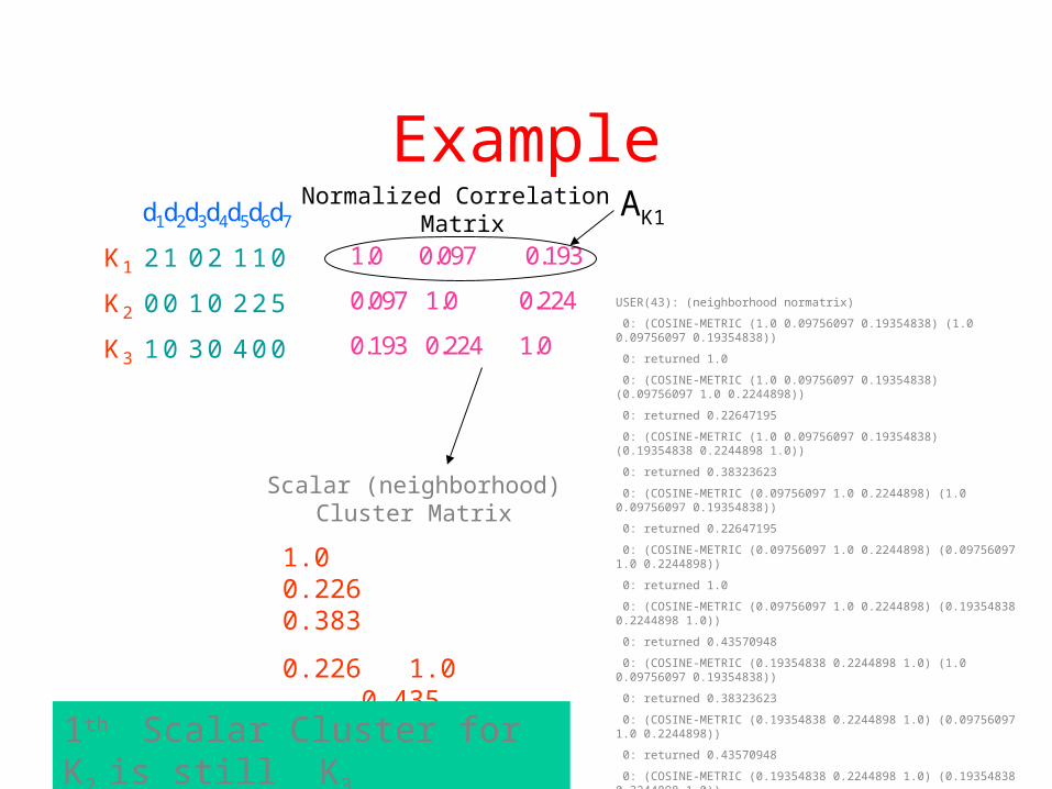
Exampled1d2d3d4d5d6d7
K1 2 1 0 2 1 1 0
K2 0 0 1 0 2 2 5
K3 1 0 3 0 4 0 0
1.0 0.097 0.193
0.097 1.0 0.224
0.193 0.224 1.0
Normalized Correlation Matrix
AK1
USER(43): (neighborhood normatrix)
0: (COSINE-METRIC (1.0 0.09756097 0.19354838) (1.0 0.09756097 0.19354838))
0: returned 1.0
0: (COSINE-METRIC (1.0 0.09756097 0.19354838) (0.09756097 1.0 0.2244898))
0: returned 0.22647195
0: (COSINE-METRIC (1.0 0.09756097 0.19354838) (0.19354838 0.2244898 1.0))
0: returned 0.38323623
0: (COSINE-METRIC (0.09756097 1.0 0.2244898) (1.0 0.09756097 0.19354838))
0: returned 0.22647195
0: (COSINE-METRIC (0.09756097 1.0 0.2244898) (0.09756097 1.0 0.2244898))
0: returned 1.0
0: (COSINE-METRIC (0.09756097 1.0 0.2244898) (0.19354838 0.2244898 1.0))
0: returned 0.43570948
0: (COSINE-METRIC (0.19354838 0.2244898 1.0) (1.0 0.09756097 0.19354838))
0: returned 0.38323623
0: (COSINE-METRIC (0.19354838 0.2244898 1.0) (0.09756097 1.0 0.2244898))
0: returned 0.43570948
0: (COSINE-METRIC (0.19354838 0.2244898 1.0) (0.19354838 0.2244898 1.0))
0: returned 1.0
1.0 0.226 0.383
0.226 1.0 0.435
0.383 0.435 1.0
Scalar (neighborhood)Cluster Matrix
1th Scalar Cluster for K2 is still K3
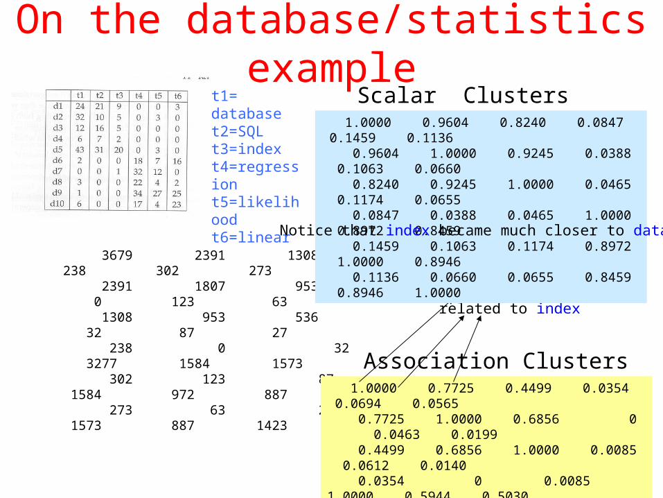
On the database/statistics examplet1= databaset2=SQLt3=indext4=regressiont5=likelihoodt6=linear
3679 2391 1308 238 302 273 2391 1807 953 0 123 63 1308 953 536 32 87 27 238 0 32 3277 1584 1573 302 123 87 1584 972 887 273 63 27 1573 887 1423
1.0000 0.7725 0.4499 0.0354 0.0694 0.0565 0.7725 1.0000 0.6856 0 0.0463 0.0199 0.4499 0.6856 1.0000 0.0085 0.0612 0.0140 0.0354 0 0.0085 1.0000 0.5944 0.5030 0.0694 0.0463 0.0612 0.5944 1.0000 0.5882 0.0565 0.0199 0.0140 0.5030 0.5882 1.0000
Association Clusters
database is most related to SQL and second most related to index
1.0000 0.9604 0.8240 0.0847 0.1459 0.1136 0.9604 1.0000 0.9245 0.0388 0.1063 0.0660 0.8240 0.9245 1.0000 0.0465 0.1174 0.0655 0.0847 0.0388 0.0465 1.0000 0.8972 0.8459 0.1459 0.1063 0.1174 0.8972 1.0000 0.8946 0.1136 0.0660 0.0655 0.8459 0.8946 1.0000
Scalar Clusters
Notice that index became much closer to database
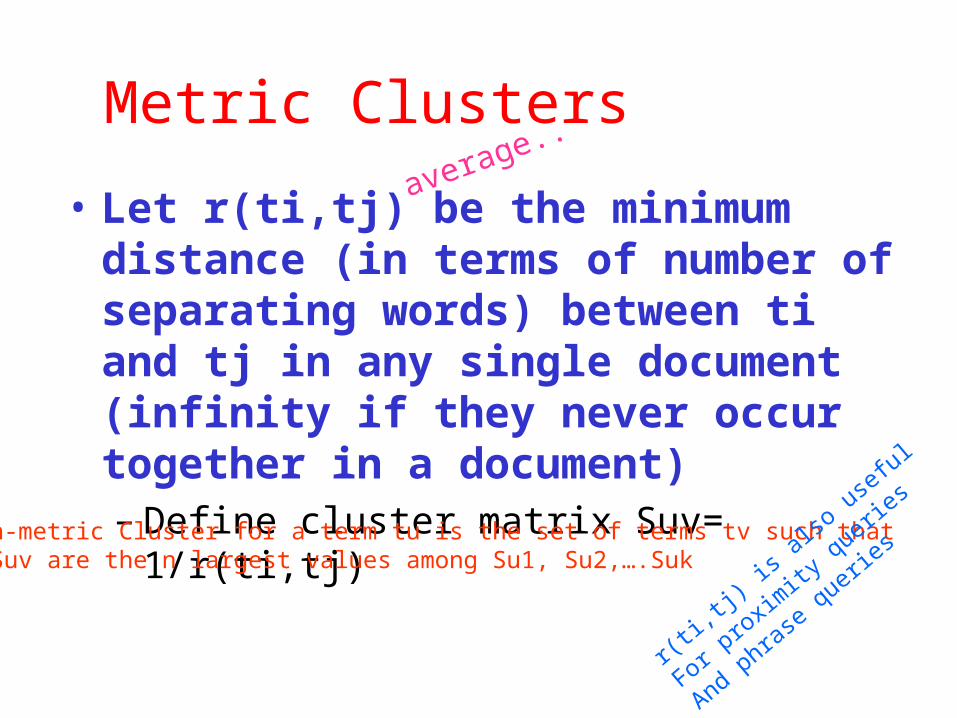
Metric Clusters
• Let r(ti,tj) be the minimum distance (in terms of number of separating words) between ti and tj in any single document (infinity if they never occur together in a document)– Define cluster matrix Suv= 1/r(ti,tj)
Nth-metric Cluster for a term tu is the set of terms tv such that Suv are the n largest values among Su1, Su2,….Suk
r(ti,tj
) is a
lso usef
ul
For proxim
ity queri
es
And phrase q
ueries
average..

Beyond Correlation analysis: PCA/LSI• Suppose I start with documents described in terms of just
two key words, u and v, but then – Add a bunch of new keywords (of the form 2u-3v; 4u-v etc), and give the
new doc-term matrix to you. Will you be able to tell that the documents are really 2-dimensional (in that there are only two independent keywords)?
– Suppose, in the above, I also add a bit of noise to each of the new terms (i.e. 2u-3v+noise; 4u-v+noise etc). Can you now discover that the documents are really 2-D?
– Suppose further, I remove the original keywords, u and v, from the doc-term matrix, and give you only the new linearly dependent keywords. Can you now tell that the documents are 2-dimensional?
• Notice that in this last case, the true dimensions of the data are not even present in the representation! You have to re-discover the true dimensions as linear combinations of the given dimensions.
– Which means the current terms themselves are vectors in the original space..
added

PCA/LSI continued• The fact that keywords in the documents are not
actually independent, and that they have synonymy and polysemy among them, often manifests itself as if some malicious oracle mixed up the data as above.
• Need Dimensionality Reduction Techniques• If the keyword dependence is only linear (as above), a general
polynomial complexity technique called Principal Components Analysis is able to do this dimensionality reduction
• PCA applied to documents is called Latent Semantic Indexing– If the dependence is nonlinear, you need non-linear dimensionality
reduction techniques (such as neural networks); much costlier.

Visual Example
• Classify Fish– Length– Height

Better if one axis accounts for most data variationWhat should we call the red axis? Size (“factor”)

We retain 1.75/2.00 x 100 (87.5%) of the original variation.
Thus, by discarding the yellow axis we lose only 12.5% of the original information.
Reduce Dimensions
• What if we only consider “size”

2/1
If you can do it for fish, why not to docs?• We have documents as vectors in the space of terms• We want to
– “Transform” the axes so that the new axes are• “Orthonormal” (independent axes)
– Notice that the new fish axes are uncorrelated..
• Can be ordered in terms of the amount of variation in the documents they capture• Pick top K dimensions (axes) in this ordering; and use these new K dimensions to do
the vector-space similarity ranking
• Why?– Can reduce noise – Can eliminate dependent variabales– Can capture synonymy and polysemy
• How?– SVD (Singular Value Decomposition)

Rank and Dimensionality• What we want to do: Given M
of rank R, find a matrix M’ of rank R’ < R such that ||M-M’|| is the smallest– If you do a bit of calculus of
variations, you will find that the solution is related to Eigen decomposition
• More specifically, Singular Value Decomposition, of a matrix
• Rank of a matrix M is defined as the size of the largest square sub-matrix of M which has a non-zero determinant. – The rank of a matrix M is also equal
to the number of non-zero singular values it has
– Rank of M is related to the true dimensionality of M. If you add a bunch of rows to M that are linear combinations of the existing rows of M, the rank of the new matrix will still be the same as the rank of M.
• Distance between two equi-sized matrices M and M’; ||M-M’|| is defined as the sum of the squares of the differences between the corresponding entries (Sum (muv-m’uv)2)– Will be equal to zero when M = M’

Bunch of Facts about SVD• Relation between SVD and Eigen value decomposition
– Eigen value decomp is defined only for square matrices• Only square symmetric matrices have real-valued eigen values• PCA (principle component analysis) is normally done on correlation matrices which are square
symmetric (think of d-d or t-t matrices).– SVD is defined for all matrices
• Given a matrix dt, we consider the eigen decomposion of the correlation matrices d-d (dt*dt’) and tt (dt’*dt). SVD is
– (a) the eigen vectors of d-d (2) positive square roots of eigen values of dd or tt (3) eigen vectors of tt» Both dd and tt are symmetric (they are correlation matrices)
– They both will have the same eigen values• Unless M is symmetric, MMT and MTM are different
– So, in general their eigen vectors will be different (although their eigen values are same)
– Since SVD is defined in terms of the eigen values and vectors of the “Correlation matrices” of a matrix, the eigen values will always be real valued (even if the matrix M is not symmetric).
• In general, the SVD decomposition of a matrix M equals its eigen decomposition only if M is both square and symmetric

Rank and Dimensionality: 2• Suppose we did SVD on a doc-
term matrix d-t, and took the top-k eigen values and reconstructed the matrix d-tk. We know– d-tk has rank k (since we zeroed
out all the other eigen values when we reconstructed d-tk)
– There is no k-rank matrix M such that ||d-t –M|| < ||d-t – d-tk||
• In other words d-tk is the best rank-k (dimension-k) approximation to d-t!
– This is the guarantee given by SVD!
• Rank of a matrix M is defined as the size of the largest square sub-matrix of M which has a non-zero determinant. – The rank of a matrix M is also equal
to the number of non-zero singular values it has
– Rank of M is related to the true dimensionality of M. If you add a bunch of rows to M that are linear combinations of the existing rows of M, the rank of the new matrix will still be the same as the rank of M.
• Distance between two equi-sized matrices M and M’; ||M-M’|| is defined as the sum of the squares of the differences between the corresponding entries (Sum (muv-m’uv)2)– Will be equal to zero when M = M’
Note that because the LSI dimensions are uncorrelated,finding the best k LSI dimensions is the same as sorting the dimensions in terms of their individual varianc (i.e., corresponding singualr values), and picking top-k

=
=
mxnA
mxrU
rxrD
rxnVT
Terms
Documents
=
=
mxn
Âk
mxkUk
kxkDk
kxnVT
k
Terms
Documents
Singular Value DecompositionConvert doc-term
matrix into 3matricesD-F, F-F, T-F
Where DF*FF*TF’ gives theOriginal matrix back
Reduce Dimensionality:Throw out low-order
rows and columns
Recreate Matrix:Multiply to produceapproximate term-document matrix.
dtk is a k-rank matrixThat is closest to dt
dt df ff tft dfk ffktfk
t
Overview of Latent Semantic Indexing
Doc-fa
ctor
(eige
n vec
tors o
f d-t*
d-t’)
factor
-facto
r
(+ve
sqrt
of ei
gen v
alues
of
d-t*d
-t’or
d-t’*
d-t;
both
same)
(term
-facto
r)T
(eige
n vec
tors o
f d-t’
*d-t)
doc
Term Term
docdtk
dxt dxf fxf fxt dxk kxk kxt dxt

-30.8998 11.4912 1.6746 -3.1330 2.2603 -1.5582
-30.3131 10.7801 0.2064 10.3670 -3.5474 -1.6751
-18.0007 7.7138 -0.8413 -5.5394 1.8438 -2.5841
-8.3765 3.5611 -0.3232 -1.9162 0.7432 -1.3505
-52.7057 20.6051 -1.7193 -2.1159 -0.6817 2.9396
-10.8052 -21.9140 5.1744 0.3599 3.0090 0.2561
-11.5080 -28.0101 -15.8265 0.1919 1.1998 0.2137
-9.5259 -17.7666 -8.7594 2.7675 4.7017 -0.3354
-19.9219 -45.0751 4.4501 -3.1140 -7.2601 -0.3766
-14.2118 -21.8263 12.0655 2.7734 6.1728 0.5132
New document coordinates d-f*f-f
t1= databaset2=SQLt3=indext4=regressiont5=likelihoodt6=linear
u =
Columns 1 through 7
-0.3994 0.1653 0.0730 -0.2327 0.1874 -0.3249 -0.1329
-0.3918 0.1551 0.0090 0.7699 -0.2941 -0.3492 0.1193
-0.2327 0.1110 -0.0367 -0.4114 0.1528 -0.5388 0.4346
-0.1083 0.0512 -0.0141 -0.1423 0.0616 -0.2816 -0.6309
-0.6813 0.2964 -0.0750 -0.1571 -0.0565 0.6129 -0.0303
-0.1397 -0.3152 0.2256 0.0267 0.2494 0.0534 0.2735
-0.1488 -0.4029 -0.6901 0.0142 0.0995 0.0445 0.2944
-0.1231 -0.2555 -0.3819 0.2055 0.3898 -0.0699 -0.4419
-0.2575 -0.6483 0.1940 -0.2312 -0.6018 -0.0785 -0.1505
-0.1837 -0.3139 0.5261 0.2060 0.5117 0.1070 0.0291
Columns 8 through 10
-0.3190 0.6715 -0.2067
-0.0165 -0.0808 -0.0136
0.3616 -0.2800 0.2264
-0.3656 -0.5904 -0.0439
0.1173 -0.1510 0.0375
0.0070 -0.2508 -0.7916
-0.4700 -0.0391 0.1347
0.5975 0.1401 -0.0521
0.1306 0.0910 0.0765
-0.1572 -0.0242 0.4991
D-F
77.3599 0 0 0 0 0
0 69.5242 0 0 0 0
0 0 22.9342 0 0 0
0 0 0 13.4662 0 0
0 0 0 0 12.0632 0
0 0 0 0 0 4.7964
0 0 0 0 0 0
0 0 0 0 0 0
0 0 0 0 0 0
0 0 0 0 0 0
-0.7352 -0.4900 -0.2677 -0.2826 -0.1831 -0.1854
0.2788 0.2351 0.1215 -0.7417 -0.3663 -0.4097
0.0413 -0.0604 -0.0741 -0.4745 -0.0473 0.8728
0.6074 -0.7156 -0.2758 0.0815 -0.1783 -0.0671
-0.0831 0.1757 0.0060 0.3717 -0.8916 0.1704
-0.0653 -0.3976 0.9121 -0.0005 -0.0568 0.0496
F-F
T-F6 singular values
(positive sqrt of eigen values of
dd or tt)
Eigen vectors of dd (dt*dt’)(Principal document
directions) Eigen vectors of tt (dt’*dt)(Principal term directions)
)2%(5.71
1
2
1
2
kloss n
ii
k
ii

For the database/regressionexample
t1= databaset2=SQLt3=indext4=regressiont5=likelihoodt6=linear
Suppose D1 is a newDoc containing “database”50 times and D2 contains“SQL” 50 times

Reconstruction (ro
unded)
With 2 LSI dimensions
Reconstruction (rounded)
With 4 LSI dimensions
24 20 10 -1 2 3 32 10 7 1 0 1 12 15 7 -1 1 0 6 6 3 0 1 0 43 32 17 0 3 0 2 0 0 17 10 15 0 0 1 32 13 0 3 -1 0 20 8 1 0 1 0 37 21 26 7 -1 -1 15 10 22
26 18 10 0 1 1 25 17 9 1 2 1 15 11 6 -1 0 0 7 5 3 0 0 0 44 31 17 0 2 1 2 0 0 19 10 11 1 -1 0 24 12 14 2 0 0 16 8 9 2 -1 0 39 20 22 4 2 1 20 11 12
Rank=2Variance loss: 7.5%
Rank=4Variance loss: 1.4%
Rank=6

LSI Ranking…• Given a query
– Either add query also as a document in the D-T matrix and do the svd OR
– Convert query vector (separately) to the LSI space– DFq*FF=q*TF
• this is the weighted query document in LSI space
– Reduce dimensionality as needed
• Do the vector-space similarity in the LSI space
TFqFFDFq
TFTFFFDFqTFq
TFFFDFqq
TFFFDFDT
I
**
'****
'**
'**

Using LSI• Can be used on the entire corpus
– First compute the SVD of the entire corpus
– Store first k columns of the df*ff matrix [df*ff]k
– Keep the tf matrix handy– When a new query q comes, take the k
columns of q*tf– Compute the vector similarity between
[q*tf]k and all rows of [df*ff]k, rank the documents and return
• Can be used as a way of clustering the results returned by normal vector space ranking– Take some top 50 or 100 of the
documents returned by some ranking (e.g. vector ranking)
– Do LSI on these documents– Take the first k columns of the
resulting [df*ff] matrix– Each row in this matrix is the
representation of the original documents in the reduced space.
– Cluster the documents in this reduced space (We will talk about clustering later)
– MANJARA did this– We will need fast SVD computation
algorithms for this. MANJARA folks developed approximate algorithms for SVD
Added based on class discussion
)'*(*)*(
)'*(*)*(
)'*'*(*)'**(
)''**(*)'**('*
)(
FFDFFFDF
DFFFFFDF
DFFFTFTFFFDF
TFFFDFTFFFDFDTDT
ncorrelatiodocdocDD
FFI

SVD Computation complexity• For an mxn matrix SVD computation is
– O( km2n+k’n3) complexity• k=4 and k’=22 for best algorithms
– Approximate algorithms that exploit the sparsity of M are available (and being developed)

Summary:What LSI can do• LSI analysis effectively does
– Dimensionality reduction
– Noise reduction
– Exploitation of redundant data
– Correlation analysis and Query expansion (with related words)
• Any one of the individual effects can be achieved with simpler techniques (see scalar clustering etc). But LSI does all of them together.

LSI (dimensionality reduction) vs. Feature Selection
• Before reducing dimensions, LSI first finds a new basis (coordinate axes) and then selects a subset of them– Good because the original axes may be too correlated to find top-k subspaces containing
most variance– Bad because the new dimensions may not have any significance to the user
• What are the two dimensions of the database example?– Something like 0.44*database+0.33*sql..
• An alternative is to select a subset of the original features themselves – Advantage is that the selected features are readily understandable by the users (to the
extent they understood the original features). – Disadvantage is that as we saw in the Fish example, all the original dimensions may have
about the same variance, while a (linear) combination of them might capture much more variation.
• Another disadvantage is that since original features, unlike LSI features, may be correlated, finding the best subset of k features is not the same as sorting individual features in terms of the variance they capture and taking the top-K (as we could do with LSI)

LSI as a special case of LDA• Dimensionality reduction (or feature
selection) is typically done in the context of specific classification tasks
– We want to pick dimensions (or features) that maximally differentiate across classes, while having minimal variance within any given class
• When doing dimensionality reduction w.r.t a classification task, we need to focus on dimensions that
– Increase variance across classes– and reduce variance within each class
• Doing this is called LDA (linear discriminant analysis)
• LSI—as given—is insensitive to any particular classification task and only focuses on data variance
– LSI is a special case of LDA where each point defines its own class
– Interestingly, LDA is also related to eigen values.
In the example above, theRed line corresponds to theDimension with most data variance
However, the green line correspondsTo the axis that does a better job ofCapturing the class variance (assumingThat the two different blobs correspondTo the different classes)

LSI vs. Nonlinear dimensionality reduction• LSI only captures linear correlations
– It cannot capture non-linear dependencies between original dimensions – E.g. if the data points are all falling on a simple manifold (e.g. a circle in the
example below), • Then, the features are “non-linearly” correlated (here X2+Y2=c)• LSI analysis can’t reduce dimensionality here
– One idea is to use techniques such as neural nets or manifold learning techniques
– Another—simpler—idea is to consider first blowing up the dimensionality of the data by introducing new axes that are nonlinear combinations of existing ones (e.g. X2, Y2, sqrt(xy) etc.)
– We can now capture linear correlations across these nonlinear dimensions by doing LSI in this enlarged space, and map the k important dimensions found back to original space.
• So, in order to reduce dimensions, we first increase them (talk about crazy!)– A way of doing this implicitly is kernel trick..
Advanced; Optional