12 - pathfinding and mazes -...

Pathfinding and mazesPathfinding and mazes

Pathfinding – problem statementPathfinding problem statement

• Finding the shortest route between two points

• How to represent the environment

• Lots of algorithmsLots of algorithms

Environment representationEnvironment representation

• Agents need to know where they can moveg y• Search space should represent either– Clear routes that can be traversed– Or the entire walkable surface

• Search space typically doesn’t represent:Small obstacles or moving objects– Small obstacles or moving objects

• Most common search space representations:– Grids– Waypoint graphs– Navigation meshes

GridsGrids

Grids as GraphsGrids as Graphs

Waypoint graphWaypoint graph

Pathfinding algorithmsPathfinding algorithms

• Random walk• Random traceRandom trace• Breadth first searchB t fi t h• Best first search

• Dijkstra’s algorithm• A* algorithm

Evaluating graph search algorithmsEvaluating graph search algorithms

• Quality of final pathi d i h• Resource consumption during search

– CPU and memory

• Whether it is a complete algorithm– A complete algorithm guarantees to find a path if one exists

Random walkRandom walk

• Agent takes a random step– If goal reached, then done

• Repeat procedure until goal reached

• Add intelligenceOnly step in cases where distance to goal is smaller– Only step in cases where distance to goal is smaller

– Stuck? With a certain probability, allow a step where distance to goal is greater

Random traceRandom trace

• Agent moves towards goalIf l h d th d– If goal reached, then done

– If obstacleT d h b l l k i• Turn around the obstacle clockwise or counter‐clockwise (pick randomly) until free path towards goal

• Repeat procedure until goal reached• Repeat procedure until goal reached

Random walk and trace propertiesRandom walk and trace properties

• Not complete algorithms

• Found paths are unlikely to be optimal

• Consume very little memoryConsume very little memory

Random walk and trace performanceRandom walk and trace performance

Search algorithmsSearch algorithms

• Breadth‐FirstBreadth First• Best‐First

ijk ’• Dijkstra’s• A* (combination of Best‐First and Dijkstra)

• Nodes represent candidate pathsNodes represent candidate paths• Keep track of numerous paths simultaneously

Breath First Search

A l d ( h d)A

B C

Closed List (Those visited)A (Path A);

D

E Open List (To be visited)F

E Open List (To be visited)B (Path A‐>B)C (Path A‐>C)

G

HH

Breath First Search

AClosed List (Those visited)A (P h A)A

B C

A (Path A);B (Path A‐>B);

D

EOpen List (To be visited)C (Path A‐>C);

FE C (Path A >C);

E (Path A‐>B‐>E);D (Path A‐>B‐>D);

G

HH

Breath First Search


B C

A (Path A);B (Path A‐>B);C (Path A‐>C);

D

EOpen List (To be visited)E (Path A‐>B‐>E);

FE E (Path A >B >E);

D (Path A‐>B‐>D);

G

HH

Breath First Search


B C


D

E

E (Path A‐>B‐>E);

Open List (To be visited)F

E Open List (To be visited)D (Path A‐>B‐>D);

G

HH

Breath First Search


B C


D

E

E (Path A‐>B‐>E);D (Path A‐>B‐>D);

FE

Open List (To be visited)G (Path A‐>B‐>D‐>G)F (P th A B D F)G

H

F (Path A‐>B‐>D‐>F)

H

Breath First Search


B C


D

E

E (Path A‐>B‐>E);D (Path A‐>B‐>D);G (Path A‐>B‐>D‐>G)

FE G (Path A >B >D >G)

Open List (To be visited)F (P th A B D F)G

H

F (Path A‐>B‐>D‐>F)H (Path A‐>B‐>D‐>G‐>H)

H

Breath First Search


B C


D

E



F (Path A‐>B‐>D‐>F)

O Li t (T b i it d)G

H

Open List (To be visited)H (Path A‐>B‐>D‐>G‐>H)

H

Breath First Search


B C


D

E



F (Path A‐>B‐>D‐>F)H (Path A‐>B‐>D‐>G‐>H) … Found!

G

H Open List (To be visited)H

Graph search algorithmsGraph search algorithms• Two lists: open and closed

• Open list keeps track of unexplored nodes

• Examine a node on the open list:– Check to see if it is the goal

If t h k it d t dd d t th li t– If not, check its edges to add more nodes to the open list• Each added node contains a reference to the node that explored it

– Place current node on closed list (mark a field as visited)

• Closed list are those that have been explored/processed and are not the goal

Node selectionNode selection

• Which open node becomes closed first?Which open node becomes closed first?– Breadth‐First processes the node that has been waiting the longestwaiting the longest

– Best‐First processes the one that is closest to the goalgoal

– Dijkstra’sprocesses the one that is the cheapest according to some weightg g

– A* chooses a node that is cheap and close to the goal

Breadth first searchBreadth first search

Best first searchBest first search

Suboptimal best first searchSuboptimal best first search

Dijkstra’s algorithmDijkstra s algorithm

• Disregards distance to goalDisregards distance to goal– Keeps track of the cost of every pathNo guessing / no search heuristic– No guessing / no search heuristic

• Computes accumulated cost paid to reach a d f th t tnode from the start

• Uses the cost (called the given cost) as a priority value to determine the next node that should be brought out of the open list

Dijkstra’ssearchDijkstra ssearch

A* algorithmA algorithm

• Admissible heuristic function that neverAdmissible heuristic function that never overestimates the true cost

• To order the open list use• To order the open list, use– Heuristic cost – estimated cost to reach the goalGi h d f h– Given cost – cost to reach node from the start

Final Cost = Given Cost + (Heuristic Cost * Heuristic Weight)

Heuristic weightHeuristic weight

• Final Cost = Given Cost + (Heuristic Cost * Heuristic Weight)( g )

• Heuristic weight controls the emphasis on the g pheuristic cost versus the given cost

• Controls the behavior of A*Controls the behavior of A– If hw=0, final cost will be the given cost ‐>DijkstraAs hw increases it behaves more like Best First– As hw increases, it behaves more like Best‐First

A* searchA search

More reading on pathfindingMore reading on pathfinding

• Amit’s A* PagesAmit s A Pages http://theory.stanford.edu/~amitp/GameProgramming/ramming/

• Beginner’s guide to pathfindinghttp://ai‐depot com/Tutorial/PathFinding htmldepot.com/Tutorial/PathFinding.html

• Waypoint graphs vs. navigation meshes h // i bl / hi /000152 h lhttp://www.ai‐blog.net/archives/000152.html

MazesMazes

Maze taken from Image‐guided maze construction, Xu and Kaplan 2007, Siggraph

Simple mazes – binary gridSimple mazes binary grid

• Matrix of booleans• ex: 21 x 21ex: 21 x 21

• Arbitrary mapping:• Arbitrary mapping:– True = black pixel = wall– False = white pixel =False white pixel open space

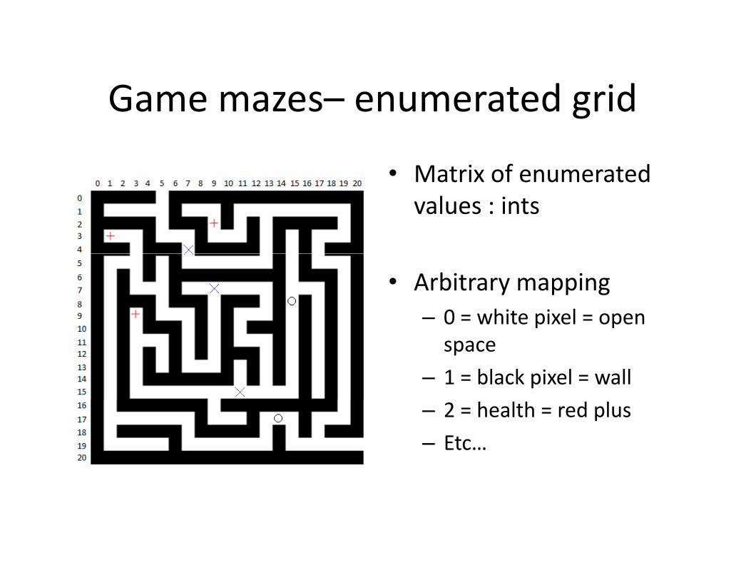
Game mazes– enumerated gridGame mazes enumerated grid

• Matrix of enumeratedMatrix of enumerated values : ints

• Arbitrary mapping– 0 = white pixel = open p pspace

– 1 = black pixel = wall– 2 = health = red plus– Etc…

Procedural maze initial valuesProcedural maze initial values

All open space – add walls All walls – add open spaceAll open space – add walls All walls add open space(usually preferred)

Advanced algorithms can also start with artist input or an image

Maze generation – start with all wallsMaze generation start with all walls

• Randomized depth first searchM k t d i it d–Mark current node as visited

–Make list of neighbors, pick one randomly– If new node is not marked as visited, remove the wall between it and its parentR i– Recursive

Maze generation – start with all wallsMaze generation start with all walls

• Randomized Kruskal's algorithmRandomized Kruskal s algorithm– Randomly select a wall that joins two unconnected open areas, and merge them

– For an n x n grid there are initially n2open areas, one per grid cell

• Randomized Prim's algorithm– Randomly pick a starting point– Keep track of walls on the boundary of the maze– Randomly select a wall that “grows” the maze

ExamplesExamples

Animation examples fromhttp://en wikipedia org/wiki/Maze generation algorithmhttp://en.wikipedia.org/wiki/Maze_generation_algorithm

Image‐based Mazes

12 - pathfinding and mazes -...

Documents