11/12/2012isc471 / hci571 isabelle bichindaritz 1 prediction
TRANSCRIPT

11/12/2012 ISC471 / HCI571 Isabelle Bichindaritz
1
Prediction
11/12/2012 ISC471 / HCI571 Isabelle Bichindaritz
2
Learning Objectives
• Analyze datasets involving predictive tasks with linear regression– Calculate predicted variables.
• Analyze datasets involving predictive tasks with nearest neighbor.
• Evaluate the prediction performance.• Interpret the analysis results.
11/12/2012 ISC471 / HCI571 Isabelle Bichindaritz
3
What Is Prediction?• Prediction is similar to classification
– First, construct a model– Second, use model to predict unknown value
• Major method for prediction is regression– Linear and multiple regression– Non-linear regression
• Prediction is different from classification– Classification refers to predicting categorical class label– Prediction models continuous-valued functions
11/12/2012 ISC471 / HCI571 Isabelle Bichindaritz
4
• Linear regression: Y = + X– Two parameters , and specify the line and are to be
estimated by using the data at hand.– using the least squares criterion to the known values of Y1,
Y2, …, X1, X2, ….
• Multiple regression: Y = b0 + b1 X1 + b2 X2.– Many nonlinear functions can be transformed into the above.
• Log-linear models:– The multi-way table of joint probabilities is approximated
by a product of lower-order tables.– Probability: p(a, b, c, d) = ab acad bcd
Regression Analysis and Log-Linear Models in Prediction
11/12/2012 ISC471 / HCI571 Isabelle Bichindaritz
5
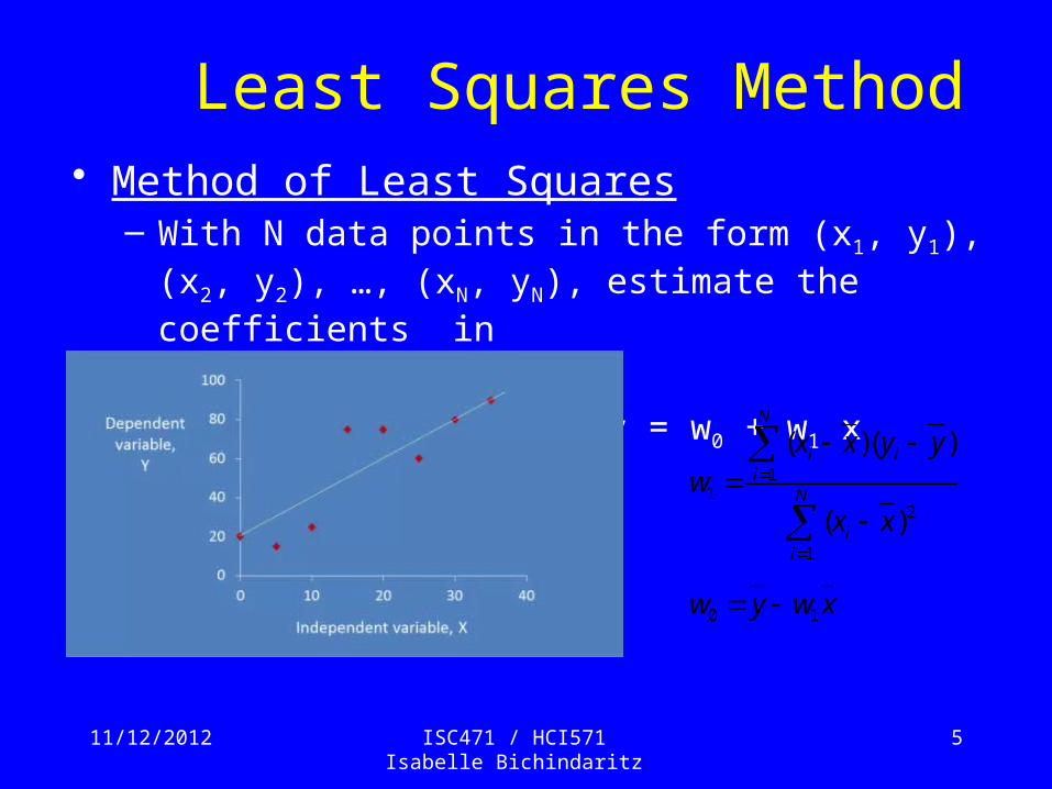
• Method of Least Squares– With N data points in the form (x1, y1), (x2, y2), …, (xN, yN),
estimate the coefficients in
y = w0 + w1 x
Least Squares Method
N
ii
i
N
ii
xx
yyxxw
1
2
11
)(
)()(
xwyw 10

11/12/2012 ISC471 / HCI571 Isabelle Bichindaritz
6
Prediction: Numerical Data
11/12/2012 ISC471 / HCI571 Isabelle Bichindaritz
7
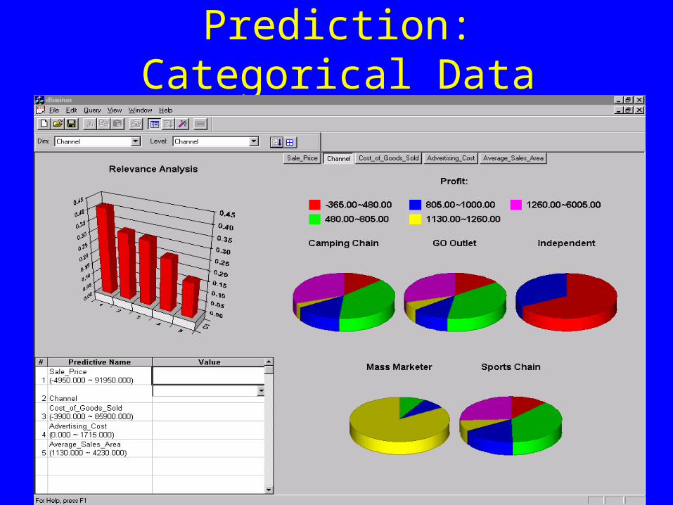
Prediction: Categorical Data

11/12/2012 ISC471 / HCI571 Isabelle Bichindaritz
8
Multivariate Data
• Multiple measurements (sensors)• d inputs/features/attributes: d-variate • N instances/observations/examples
Nd
NN
d
d
XXX
XXX
XXX
21
222
21
112
11
X
11/12/2012 ISC471 / HCI571 Isabelle Bichindaritz
9
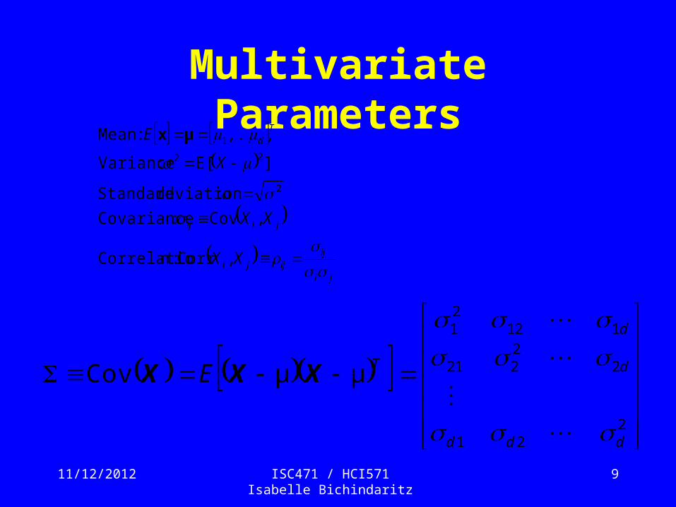
Multivariate Parameters
ji
ijijji
jiij
Td
XX
XX
X
E
,Corr :nCorrelatio
,Cov:Covariance
:deviation Standard
]E[:Variance
,...,:Mean
2
22
1μx
221
22221
11221
Cov
ddd
d
d
TE
μμ XXX
11/12/2012 ISC471 / HCI571 Isabelle Bichindaritz
10
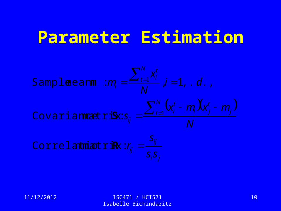
Parameter Estimation
ji
ijij
jtj
N
t iti
ij
N
t
ti
i
ss
sr
N
mxmxs
diN
xm
:matrix n Correlatio
:matrix Covariance
,...,1,:mean Sample
1
1
R
S
m

11/12/2012 ISC471 / HCI571 Isabelle Bichindaritz
11
Estimation of Missing Values• What to do if certain instances have missing
attributes?• Ignore those instances: not a good idea if the
sample is small• Use ‘missing’ as an attribute: may give
information• Imputation: Fill in the missing value
– Mean imputation: Use the most likely value (e.g., mean)
– Imputation by regression: Predict based on other attributes
11/12/2012 ISC471 / HCI571 Isabelle Bichindaritz
12
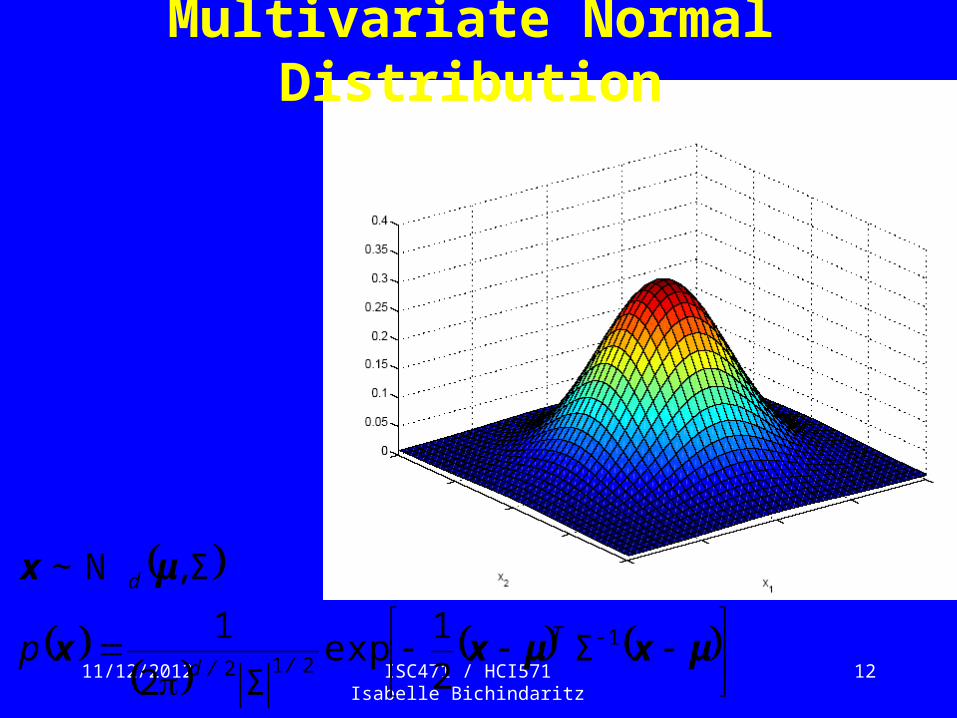
Multivariate Normal Distribution
μxμxx
μx
1212 2
1exp
2
1Σ
Σ
Σ
T
//d
d
p
~ ,N
11/12/2012 ISC471 / HCI571 Isabelle Bichindaritz
13
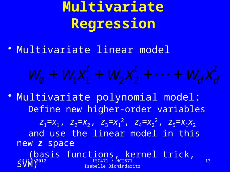
Multivariate Regression
• Multivariate linear model
• Multivariate polynomial model: Define new higher-order variables
z1=x1, z2=x2, z3=x12, z4=x2
2, z5=x1x2
and use the linear model in this new z space (basis functions, kernel trick, SVM)
tdd
tt xwxwxww 22110
11/12/2012 ISC471 / HCI571 Isabelle Bichindaritz
14
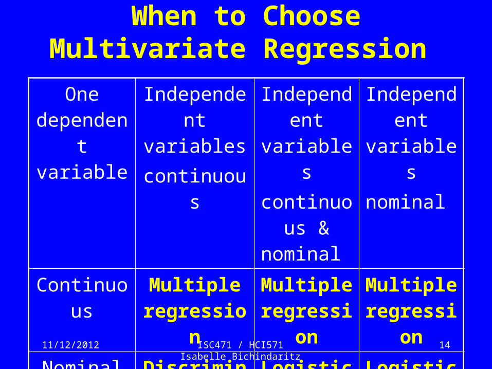
When to Choose Multivariate Regression
One dependent variable
Independent variables
continuous
Independent variables
continuous & nominal
Independent variablesnominal
Continuous Multiple regression
Multiple regression
Multiple regression
Nominal Discriminant analysis
Logistic regression
Logistic regression
11/12/2012 ISC471 / HCI571 Isabelle Bichindaritz
15
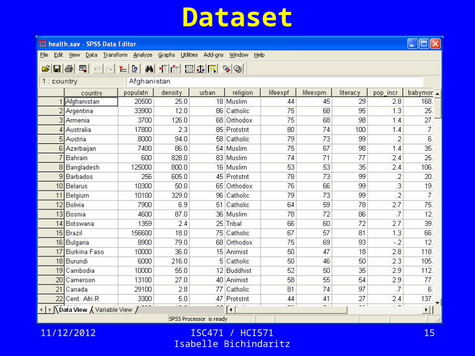
Dataset
11/12/2012 ISC471 / HCI571 Isabelle Bichindaritz
16
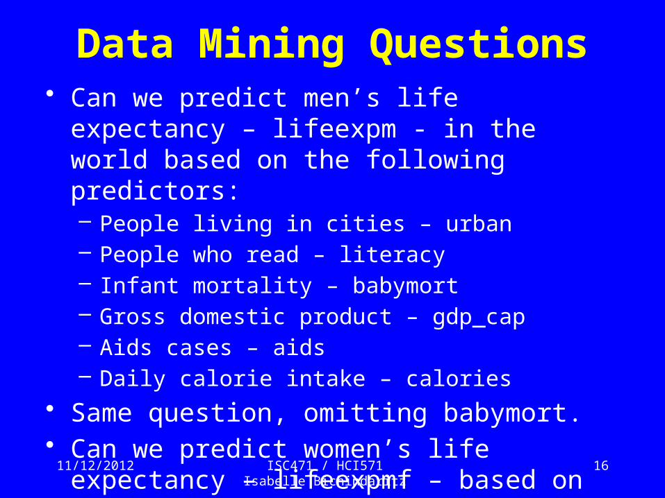
Data Mining Questions• Can we predict men’s life expectancy – lifeexpm -
in the world based on the following predictors:– People living in cities – urban– People who read – literacy– Infant mortality – babymort– Gross domestic product – gdp_cap– Aids cases – aids– Daily calorie intake – calories
• Same question, omitting babymort.• Can we predict women’s life expectancy –
lifeexpmf – based on lifeexpmm and the previous predictors.
11/12/2012 ISC471 / HCI571 Isabelle Bichindaritz
17
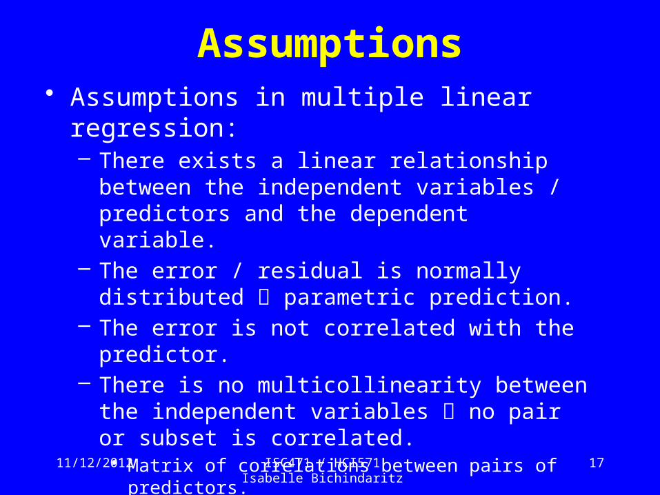
Assumptions• Assumptions in multiple linear regression:
– There exists a linear relationship between the independent variables / predictors and the dependent variable.
– The error / residual is normally distributed parametric prediction.
– The error is not correlated with the predictor.– There is no multicollinearity between the independent
variables no pair or subset is correlated.• Matrix of correlations between pairs of predictors.
11/12/2012 ISC471 / HCI571 Isabelle Bichindaritz
18
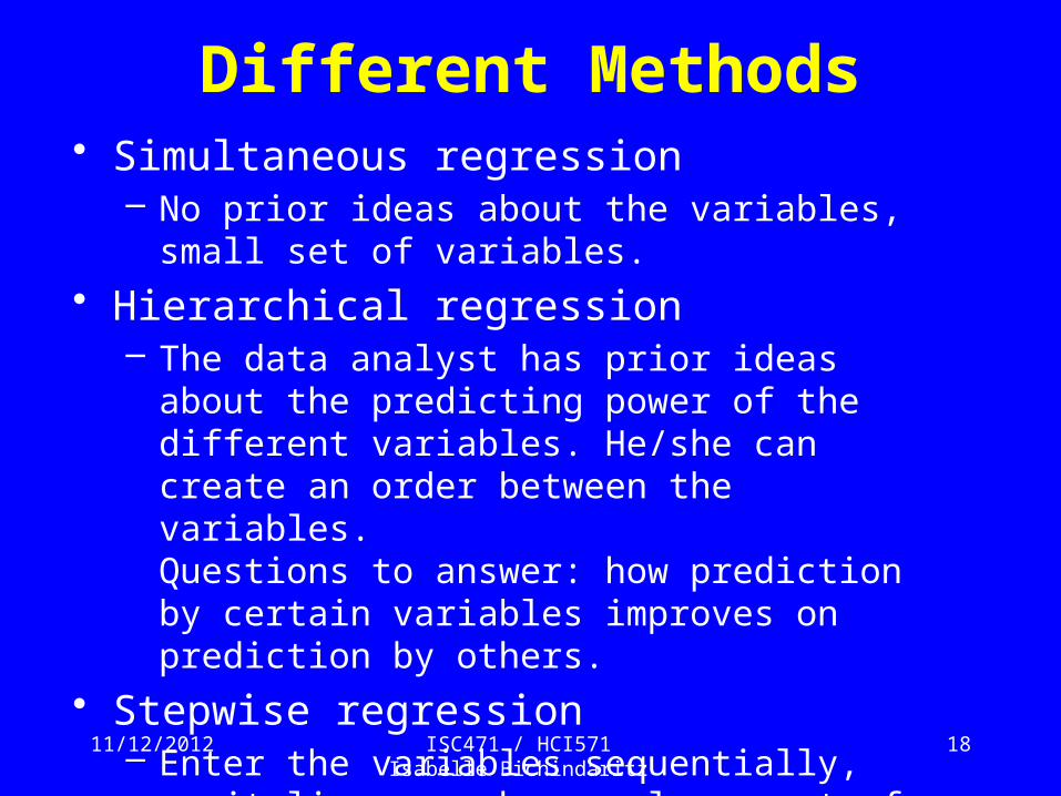
Different Methods• Simultaneous regression
– No prior ideas about the variables, small set of variables.
• Hierarchical regression– The data analyst has prior ideas about the predicting
power of the different variables. He/she can create an order between the variables. Questions to answer: how prediction by certain variables improves on prediction by others.
• Stepwise regression– Enter the variables sequentially, capitalizes on chance,
large set of variables – not recommended.

11/12/2012 ISC471 / HCI571 Isabelle Bichindaritz
19
Simultaneous Method• Question: can we predict lifeexpm based on the
following predictors: urban, literacy, babymort, gdp_cap, aids, calories?
• Enter all the variables simultaneously.
• Study the relative contribution of each variable to the prediction.

11/12/2012 ISC471 / HCI571 Isabelle Bichindaritz
20
Check the Assumptions
• In SPSS, several assumptions can be checked during analysis by requesting
– Correlation matrix pairwise collinearity
– Coefficients table Multicollinearity consider combining these variables
– Study scatterplots of the data and look for linear relationships between each predictor and the dependent variable …

11/12/2012 ISC471 / HCI571 Isabelle Bichindaritz
21
Collinearity• Can be checked before regression analysis too.• Analyze correlate bivariate
select the independent variables urban, literacy, babymort, gdp_cap, aids, caloriesselect Options missing values exclude cases listwise.Click Continue OK
• Pearson correlation coefficient:– r > 0.5 or r < 0.5 and significant at p < 0.05 – Eliminate correlations greater than 0.9 or smaller than
-0.9 , if significant.

11/12/2012 ISC471 / HCI571 Isabelle Bichindaritz
22
Collinearity
11/12/2012 ISC471 / HCI571 Isabelle Bichindaritz
23
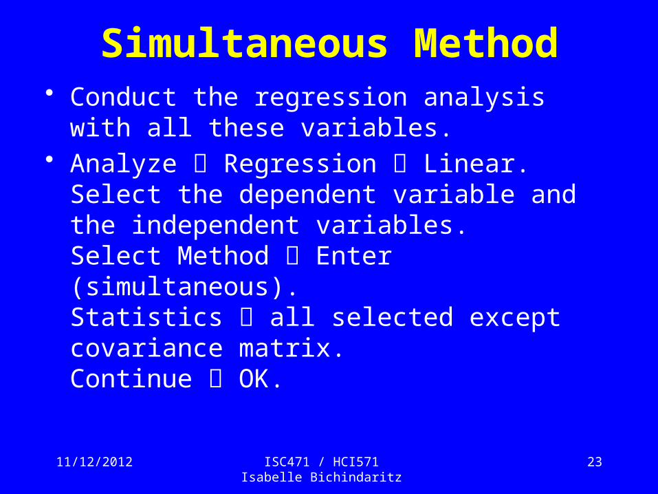
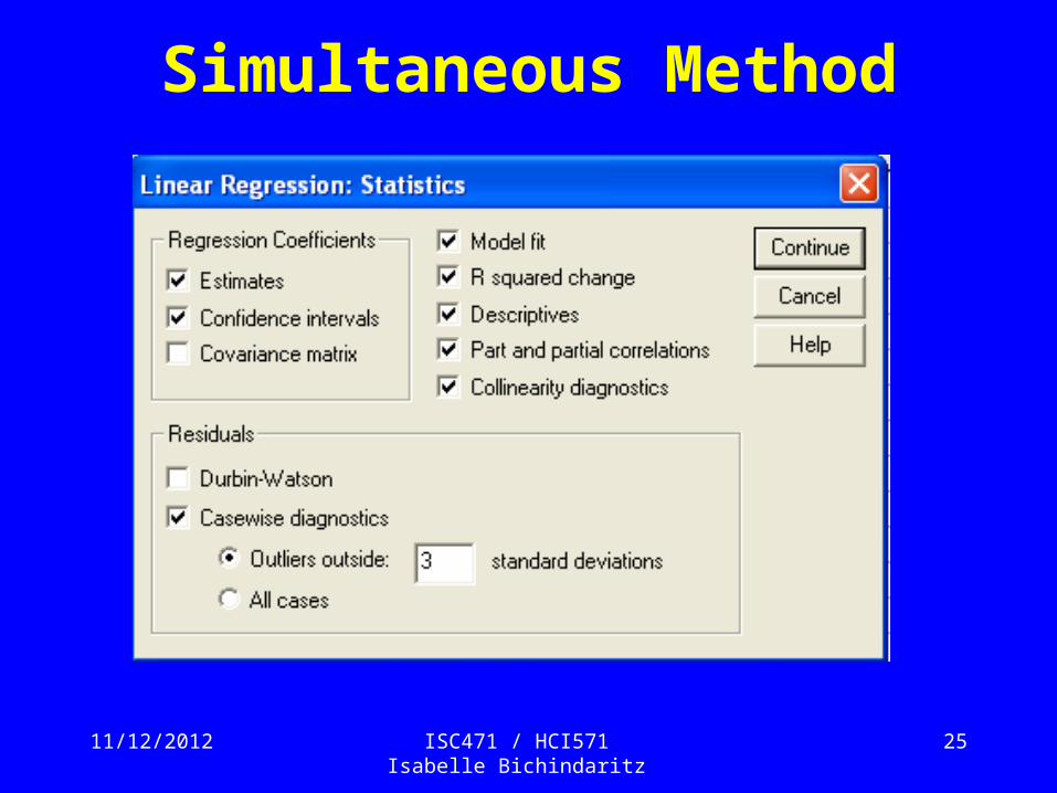
Simultaneous Method• Conduct the regression analysis with all these
variables.• Analyze Regression Linear.
Select the dependent variable and the independent variables.Select Method Enter (simultaneous).Statistics all selected except covariance matrix.Continue OK.

11/12/2012 ISC471 / HCI571 Isabelle Bichindaritz
24
Simultaneous Method
11/12/2012 ISC471 / HCI571 Isabelle Bichindaritz
25
Simultaneous Method
11/12/2012 ISC471 / HCI571 Isabelle Bichindaritz
26
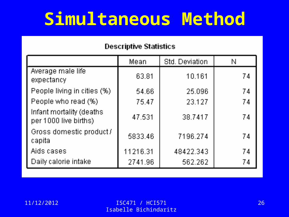
Simultaneous Method
11/12/2012 ISC471 / HCI571 Isabelle Bichindaritz
27
Simultaneous Method
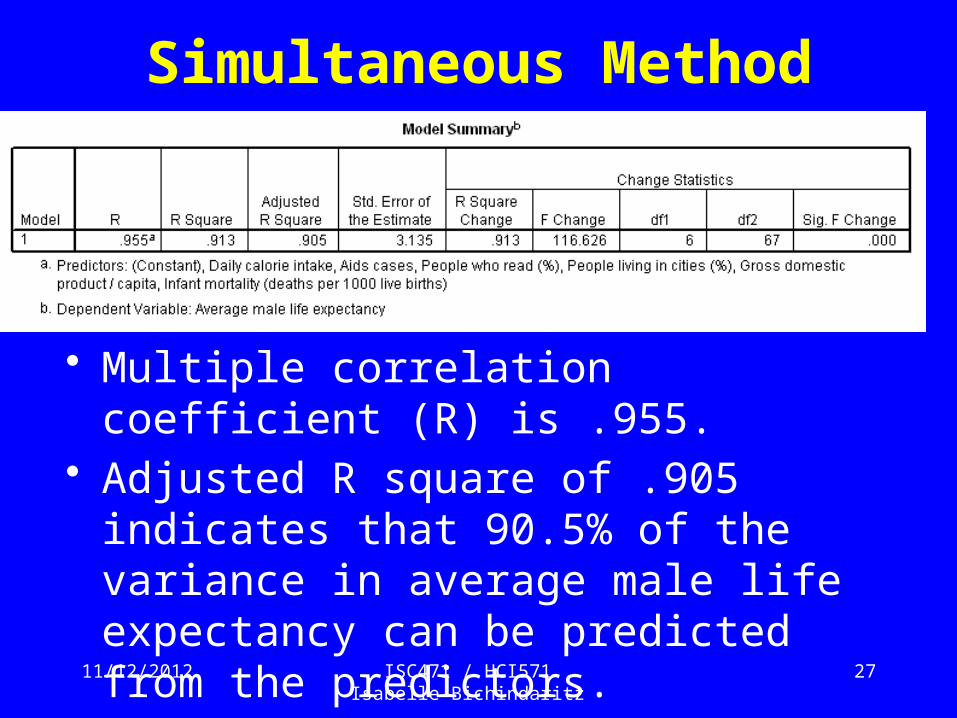
• Multiple correlation coefficient (R) is .955.• Adjusted R square of .905 indicates that
90.5% of the variance in average male life expectancy can be predicted from the predictors.
• Maybe some predictors are not helping.

11/12/2012 ISC471 / HCI571 Isabelle Bichindaritz
28
Simultaneous Method
• ANOVA (ANalysis Of VAriance) indicates with F= 116.626 that the predictors significantly predict the dependent variable – greater than 1.0 at least.
• Tests the fit of the model to the data.
11/12/2012 ISC471 / HCI571 Isabelle Bichindaritz
29
Simultaneous Method
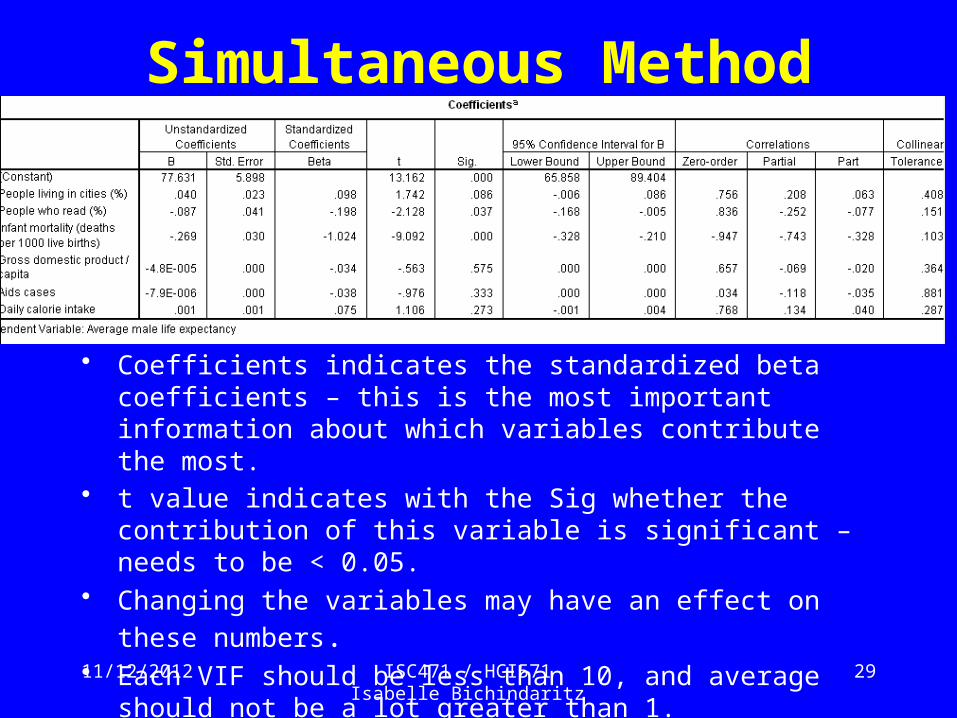
• Coefficients indicates the standardized beta coefficients – this is the most important information about which variables contribute the most.
• t value indicates with the Sig whether the contribution of this variable is significant – needs to be < 0.05.
• Changing the variables may have an effect on these numbers. • Each VIF should be less than 10, and average should not be a lot
greater than 1.• If tolerance is < 1-R2 = .095, then there is a risk of multicollinearity.
This is not the case here for any variable.
11/12/2012 ISC471 / HCI571 Isabelle Bichindaritz
30
Simultaneous Method
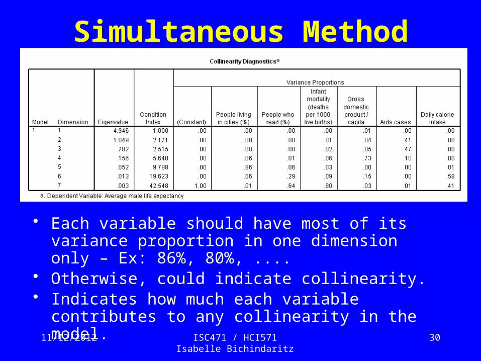
• Each variable should have most of its variance proportion in one dimension only – Ex: 86%, 80%, ....
• Otherwise, could indicate collinearity.• Indicates how much each variable contributes to any
collinearity in the model.

11/12/2012 ISC471 / HCI571 Isabelle Bichindaritz
31
Regression Result• Question: can we predict lifeexpm based on the
following predictors: urban, literacy, babymort, gdp_cap, aids, calories?
• AnswerMultiple regression was conducted to determine the best linear combination of urban, literacy, babymort, gdp_cap, aids, and calories for predicting lifeexpm. The descriptive statistics and correlations can be found in table …. and indicate a strong correlation between babymort and literacy.

11/12/2012 ISC471 / HCI571 Isabelle Bichindaritz
32
Regression Result• This combination of variables significantly
predicted lifeexpm, F(6, 73) = 118.626, p < 0.000. Only literacy and babymort significantly contributed to the prediction. The beta weights, presented in table … suggest that babymort contributes the most to predicting lifeexpm, and that literacy also contributes to this prediction. The adjusted R squared value was .905, which indicates that 90.5% of the variance in lifeexpm was explained by the model. This is a very large effect.
33
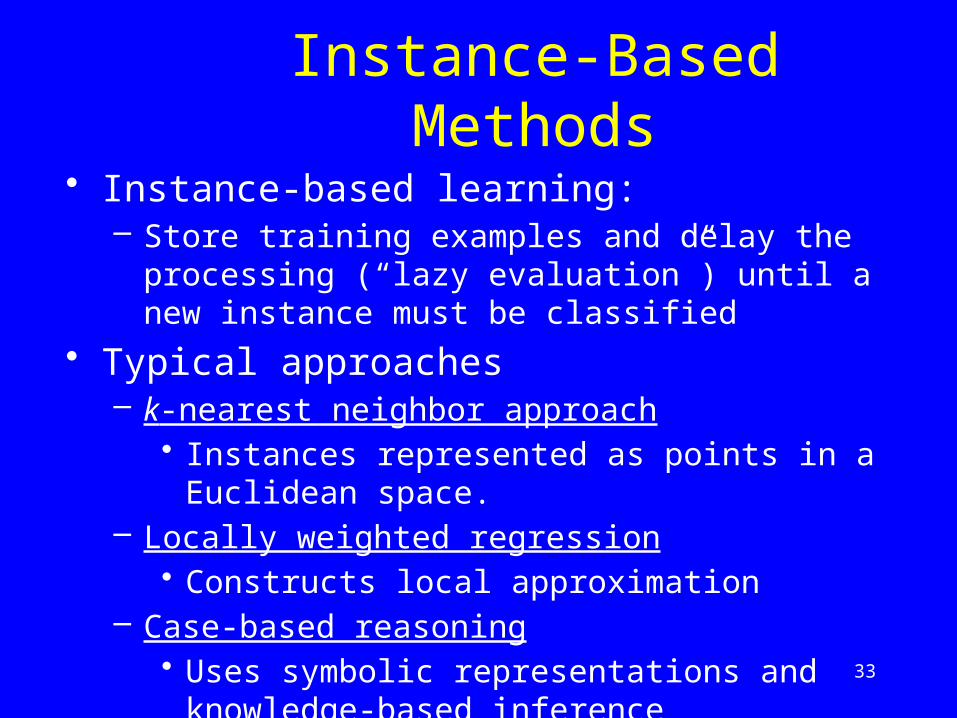
Instance-Based Methods
• Instance-based learning: – Store training examples and delay the processing (“lazy
evaluation”) until a new instance must be classified
• Typical approaches– k-nearest neighbor approach
• Instances represented as points in a Euclidean space.– Locally weighted regression
• Constructs local approximation– Case-based reasoning
• Uses symbolic representations and knowledge-based inference
34
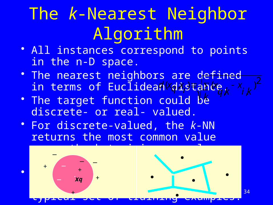
The k-Nearest Neighbor Algorithm
• All instances correspond to points in the n-D space.• The nearest neighbors are defined in terms of
Euclidean distance.• The target function could be
discrete- or real- valued.• For discrete-valued, the k-NN returns the most
common value among the k training examples nearest to xq.
• Vonoroi diagram: the decision surface induced by 1-NN for a typical set of training examples.
.
_+
_ xq
+
_ _+
_
_
+
.
..
. .
k
kix
kqxixqxd 2)
,,(),(

35
Discussion on the k-NN Algorithm• The k-NN algorithm for continuous-valued target
functions– Calculate the mean values of the k nearest neighbors
• Distance-weighted nearest neighbor algorithm– Weight the contribution of each of the k neighbors according
to their distance to the query point xq
• giving greater weight to closer neighbors– Similarly, for real-valued target functions
• Robust to noisy data by averaging k-nearest neighbors• Curse of dimensionality: distance between neighbors
could be dominated by irrelevant attributes. – To overcome it, axes stretch or elimination of the least
relevant attributes.
wd xq xi
12( , )

36
The k-Nearest Neighbor Algorithm
• This algorithm can be used for classification tasks– Example: word pronunciation
http://videolectures.net/aaai07_bosch_knnc/
• Or for prediction tasks.