1

1.1 Introduction

The objective of this report was to develop algorithms for optimization of leastsquare best fit geometry for various geometric elements. The matlab code implementationwas done for the various geometries and tested with the real data points obtained fromco-ordinate measuring machines. The various geometries that were studied here are asfollows:

Lines in a specified planeLines in three dimensionPlanesCircles in a specified planeSpheres andCylinders

This report was written in such a way that someone who has some knowledge ofLinear Algebra and curve fitting could easily follow. The concise abstract of variouspapers that the authors referred is given as Appendix 1 and 2. It is advised to go throughthe Appendix before starting to read the report. The least square best-fit referenceelement to Cartesian data points was only established in this report.

1.2.Least Squares Best Fit Element

The application of least square criteria can be applied to a wide range of curvefitting problems. Least square best-fit element to data is explained by taking the problemof fitting the data to a plane.

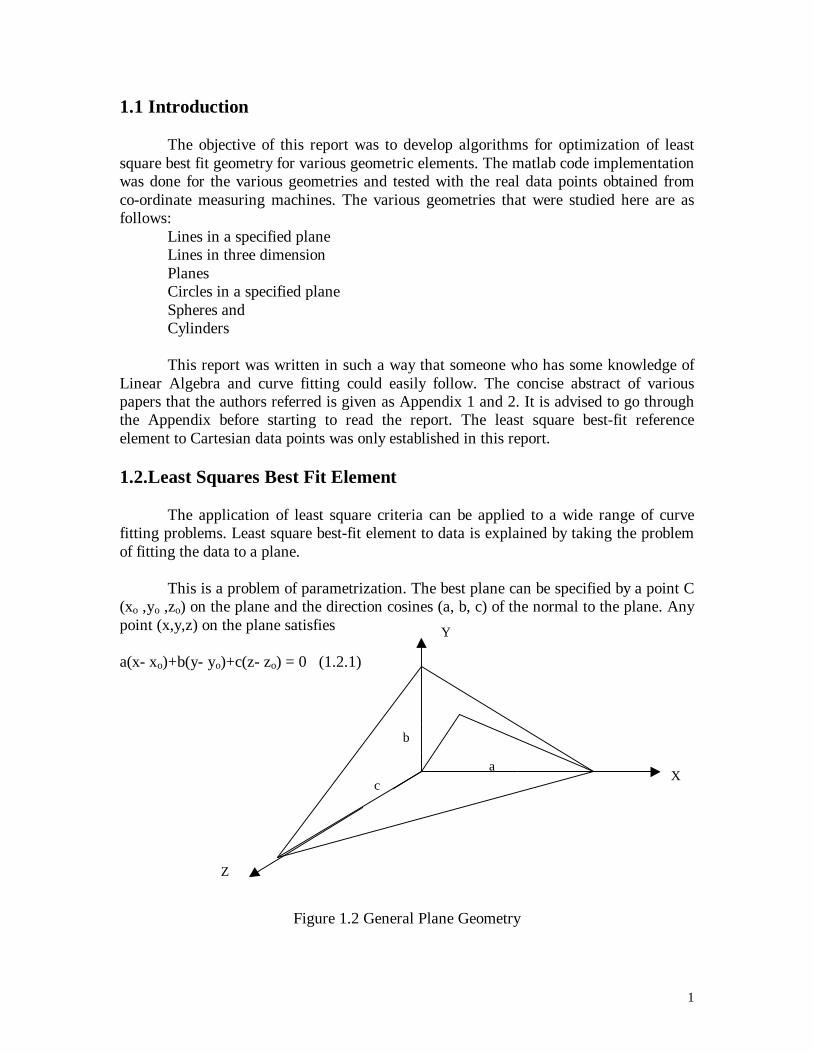
This is a problem of parametrization. The best plane can be specified by a point C(xo ,yo ,zo) on the plane and the direction cosines (a, b, c) of the normal to the plane. Anypoint (x,y,z) on the plane satisfies

a(x- xo)+b(y- yo)+c(z- zo) = 0 (1.2.1)

Figure 1.2 General Plane Geometry

b

ac

X

Y

Z

2

The distance from any point A (xi ,yi, zi ) to a plane specified above is given by

di = a(xi - xo)+b(yi - yo)+c(zi - zo) (1.2.2)

The sum of squares of distances of each point from the plane is

F = i

n

=∑

1 di

2 (1.2.3)

Hence our problem is to find the parameters (xo ,yo ,zo) and (a,b,c) that minimizes thesum F.

1.3 Optimization

Consider a function

E(u) = i

n

=∑

1 di

2(u) (1.3.1)

which has to be minimized with respect to the parameters u = ( u1 … . un)T

Here in this case di represents the distance of the data point to the geometric elementparameterized by u.

1.3.1 Linear Least Squares

The conventional approach used in the standard textbooks for least square fitting of astraight line is described below for the understanding. The matrix formulation of theproblem is also explained in detail, as it is very useful when solving large problems.

Consider fitting a straight liney = a + bx (1.3.1.1)

through a set of data points ( , )x yi i , i=1 to n. The minimizing function minimizes thesum of the squares of the distances of the points from the straight line measured in thevertical direction. Thus

F yi a bxii

n= − −

=∑ ( )2

1 (1.3.1.2)

is the minimizing function. A necessary condition for f to be minimum is∂∂fa

= 0 and ∂∂fb

= 0 (1.3.1.3)

Thus partial differentiation of the above function with respect to a and b gives

3

2 1 0

2 0

1

1

( ) ( )

( ) ( )

− − − =

− − − =

=

=

∑

∑

y a bx

x y a bx

i ii

n

i i ii

n (1.3.1.4)

These can be simplified as

y na b x

x y a x b x

i ii

n

i

n

i i ii

n

ii

n

i

n

= +

= −

==

= ==

∑∑

∑ ∑∑11

1

2

11

(1.3.1.5)

The equations above can be solved simultaneously to give us the values for a and b.

1.3.2 Normal equation

Consider to fit a straight line, y = a+bx, to the set of data (x1,y1), (x2,y2),… , (xn,yn). If the data points were collinear, the line would pass through n point. So

y1 = a + bx1 (1.3.2.1)y2 = a + bx2

y3 = a + bx3

Myn = a + bxn

It can be written in a matrix form

=

ba

x1

x1x1

y

yy

n

2

1

n

2

1

MMM(1.3.2.1)

Let B =

n

2

1

y

yy

M, A =

n

2

1

x1

x1x1

MM , and p=

ba

(1.3.2.2)

So it can be compacted as B=AP

The objective is to find a vector p that minimizes the Euclidean length of the difference

||B-AP||

4

if P=P* =

*

*

ba

is a minimize vector, y =a* + b*x is a least square straight-line fit. This

can be explained as

||B-AP||2 = (y1 - a - bx1)2 + (y2 - a - bx2)2 + … + (yn - a - bxn)2 (1.3.3.3)

if let d1 = (y1 - a - bx1)2 , d2 = (y2 - a - bx2)2 , … , dn = (yn - a - bxn)2

d can be explained as the distance from a point of a data set to a fitting line. So

||B-AP||2 = 2n

22

21 d dd +++ L (1.3.3.4)

Figure 1.3.3 Finding Normal Equation

To minimize ||B-AP||, AP must be equal to AP* where AP* is the orthogonal projection ofB on the column space of A. This implies B - AP* must be orthogonal to the columnspace of A. So

(B - AP*)AP = 0 for every vector P in R2

This can be written as

(AP)T(B - AP*) = 0

PTAT (B - AP*) = 0

PT (ATB - ATAP*) = 0

(ATB - ATAP*)P = 0

So ATB - ATAP* is orthogonal to every vector P in R2. This implies

ATB - ATAP* = 0

B

B - AP

B - AP*

AP*

APColumn spaceA in Rn

5

ATAP = ATB

Which implies that P* satisfies the linear system

ATAP = ATB (1.3.3.5)

This equation is called as Normal equation. This will provide the solution for p as

P = (ATA)-1ATB (1.3.3.6)

This equation can be used in the case of least square fit of a polynomial.

1.3.3 Eigen Vectors and Singular Value Decomposition

From equation (1.3.3.6), (ATA)-1 is very difficult to solve. So the alternativemethod using singular value decomposition is used to solve P

Singular Value Decomposition

A matrix can be decomposed in 3 matrices

A = USVT (1.3.3.1)

Where U and V are orthogonal matrices, and S is a diagonal matrix containing thesingular matrix of A

Place A =USVT into the normal equation

(USVT)T(USVT)P = (USVT)TB

(VSTUTUSVT)P = VSTUTBknowing that

UTU =I UT = U-1 VTV = I VT = V-1

So (VSTSVT)P = VSTUTB

Multiplying both sides by V-1

(STSVT)P = STUTB

S is a diagonal matrix; therefore, (SSVT)P =SUTB

Multiplying both sides by S-1 2 times

6

VTP = S-1UTBAgain multiplying both sides by V*

VVTP = VS-1UTBSo the solution for P is

P=VS-1UTB (1.3.3.2)

1.3.4 Gauss-Newton Algorithm

Newton's method is one of the most powerful and well-known numerical methodsfor solving a root finding problem f(x)=0 where f(x) is a non-linear function. Thistechnique is used in applications of linear least squares model of circle, sphere, cylinder,and cones. To motivate how such an algorithm works, first the Newton method isdescribed.

Suppose that given a function f that its domain is [a,b] , and let ∈x [a,b] such thatf'( x ) ≠ 0. The Taylor polynomial expansion for f(x) about x is

(x))('f'2

2)x-(x )x()f'x-(x )xf(f(x) ξ++= (1.3.4.1)

where ]x[x, (x)∈ξ .

Since f(q) = 0 where q=x, it gives

(x))('f'2

2)x-(x )x()f'x-(x )xf(0 ξ++=

Newton's method is assumed as |q- x | is small. Therefore (p- x )2 is much small. So

)x()f'x-(q )xf(0 +=

(x)f')xf( - )x-(q =

Let q = u1 , x = u0, and p =(x)f'

)xf( -

Therefore u1 = u0 + p and p = )(uf')f(u

- 0

0 (1.3.4.2)

7

Figure 1.3.4 The iteration of Newton's method

From figure 1.3.4, the root finding problem y = f(u) can be done by following steps:1) f(u0) and f'(u0) are evaluated2) a tangent line to graph at the point (u0, f(u0)) is found. It cuts the u axis at u1

3) find point u1, and draw a tangent to graph at the point u1 to find point u24) these steps above are repeated until it is converged (close to u*)

The main ingredients of the algorithm area) given an approximate solution, the problem is linearisedb) the linear version of the problem is solvedc) the solution of the linear problem is used to update estimate of the solution.

In the linear least square problem, the measurement of how well the geometric elementfits a set of data point can be determined

E = ∑n

1

2id (1.3.4.2)

Where di is a distance from the point to the geometric element.

In the case, di is not linear function; the Gauss - Newton algorithm is used for finding theminimum of a sum of squares E. Assuming there is one initial estimate u*, solve a linearleast squares system of the form

(u0,f(u0))

u0

u1

(u1,f(u1))

f'(u1)

f'(u0)

y =f(u)y

uu2

8

Jp = -d (1.3.4.3)

Where J is the m×n Jacobean matrix whose ith row is the gradient of di with respect to theparameter u, i.e.,

Jij = j

i

ud

∂∂

(1.3.4.4)

It's evaluated at u, and the ith component of d is di(u). The parameter is updated as

u:= u+p (1.3.4.5)

Converged conditions

Steps of Newton's algorithm are repeated until it reaches to a convergent point. Here 3criteria are relevant for testing for convergence:

1) the change of E should be small2) the size of the update, for instance (pTp)1/2, must be small3) the partial derivation of E with respect to the optimization parameters, for instance

(ggT)1/2 where g=JTd, should be small.

2. Least Square Best Fit Line

Lines can be in a specified plane (2 Dimensional) or 3 dimensional. Since the 2 Dline is a particular case of 3 dimensional line, the 3D line is discussed in detail. Theprocedure to fit a line to m data points(xi, yi,,zi ), where m≥2, is given below.Any point (x,y,z) on the line satisfies

(x,y,z) = (xo, yo,,zo ) + t (a, b, c) (2.1) for some value of t.

It is known that the distance from a point to a line in 3 dimension asdi = √[ui

2+ vi2+ wi

2 ] (2.2)

2.1 Parametrization

A line can be specified byi) a point (xo, yo,,zo ) on the line andii) the direction cosines (a, b, c).

9

2.2 Algorithm Description

The best-fit line passes through the centroid ( x , y , z ) of the data and this specifies apoint on L also the direction cosines have to be found out.

i)The first step is to find the average of the points x, y and z.

x = Σ xi,/n (2.2.1)y = Σ yi,/nz = Σ zi, /n

ii) The matrix A is formulated such that its first column is xi – x , second columnyi –y and third column zi- z

iii) This matrix A is solved by singular value decomposition. The smallest singular valueof A is selected from the matrix and the corresponding singular vector is chosen whichthe direction cosines (a, b, c)

iv) The best-fit plane is specified by x , y , z , a, b and c.

3 Least Square Best Fit Plane

The procedure to fit a plane to m data points(xi yI,,zi), where m≥3, is given below.Any point (x,y,z) on the plane satisfies

a(x-xo)+b(y-yo )+c(z-zo )=0. (3.1)

It is known that the distance from a point (xi yi, zi) to a plane specified by xo, yo,,zo ,a, band c is given by

di = a(x-xo)+b(y-yo )+c(z-zo ) (3.2)

3.1 Parametrization

A plane can be specified byiii) a point (xo, yo,,zo ) on the plane andiv) the direction cosines (a, b, c) of the normal to the plane

3.2 Algorithm Description

The best-fit plane passes through the centroid (xbar, ybar, zbar) of the data and thisspecifies a point on P also the direction cosines have to be found out.For this, (a,b,c) is the eigen vector associated with the smallest eigen value ofB = ATA

i)The first step is to find the average of the points x, y and z.

10

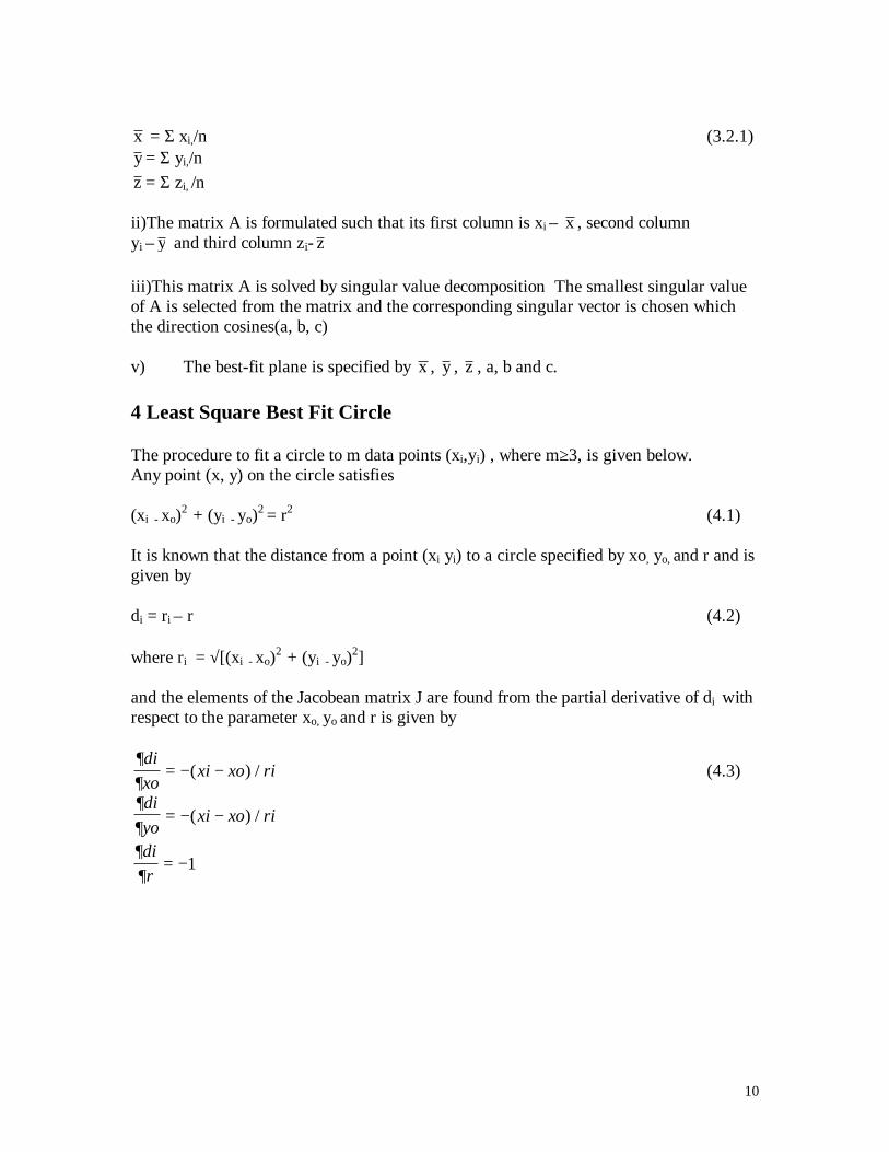
x = Σ xi,/n (3.2.1)y = Σ yi,/nz = Σ zi, /n

ii)The matrix A is formulated such that its first column is xi – x , second columnyi –y and third column zi- z

iii)This matrix A is solved by singular value decomposition The smallest singular valueof A is selected from the matrix and the corresponding singular vector is chosen whichthe direction cosines(a, b, c)

v) The best-fit plane is specified by x , y , z , a, b and c.

4 Least Square Best Fit Circle

The procedure to fit a circle to m data points (xi,yi) , where m≥3, is given below.Any point (x, y) on the circle satisfies

(xi - xo)2 + (yi - yo)2 = r2 (4.1)

It is known that the distance from a point (xi yi) to a circle specified by xo, yo, and r and isgiven by

di = ri – r (4.2)

where ri = √[(xi - xo)2 + (yi - yo)2]

and the elements of the Jacobean matrix J are found from the partial derivative of di withrespect to the parameter xo, yo and r is given by

∂∂

dixo

xi xo ri= − −( ) / (4.3)

∂∂

diyo

xi xo ri= − −( ) /

∂∂dir

= − 1

11

4.1 Parameterization

A circle can be specified byi) its center (xo, yo) andii) its radius r.

4.2 Algorithm Description

The algorithm that is used to find the best-fit circle is Gauss-Newton algorithm, which isexplained already. First the initial estimates are to be found then the Gauss-Newtonalgorithm is implemented. The initial estimates of the center and radius of the circle aremade by solving the problem as a linear least square model. The steps that are followedare as follows

i) Minimization of F

F = f i

2

i=1

m

∑ (4.2.1)

where

f i = −r ri2 2

.

ii)This can be reduced to a linear system in x0, y0and ρ as,

( ) ( )( )

f i = − + − −

= − − + + − + +

x x y y r

x x y y x y r x y

i i

i i i i

0

2

0

2 2

0 0 02

02 2 2 22 2

,

( ), (4.2.2)where ρ isx y r0

202 2+ − .

iii)For minimizing F, the linear least squares system is solved

Axy b

0

0

ρ

=

where the elements of the ith row of A are the coefficients (2xi,2yi,-1) and theith element of b is

x yi i2 2+ .

iv) An estimate of r is obtained from the equation of ρ.

Once the initial estimates are obtained the right hand side vector d and Jacobean matrix Jare formed.

(4.2.3)

12

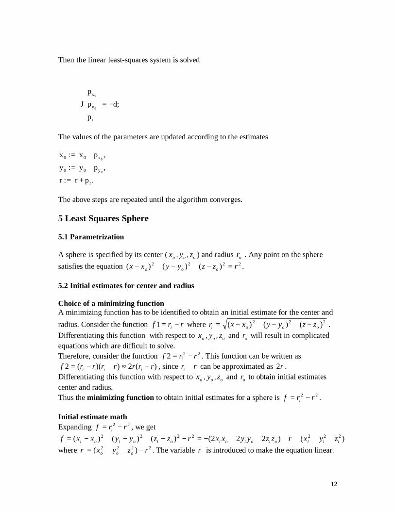
Then the linear least-squares system is solved

J

p

p

p

d;x

y

r

0

0

= −

The values of the parameters are updated according to the estimates

x := x p

y := y p

r := r + p

0 0 x

0 0 y

r

0

0

++

,

,

.

The above steps are repeated until the algorithm converges.

5 Least Squares Sphere

5.1 Parametrization

A sphere is specified by its center ( xo , yo , zo ) and radius ro . Any point on the spheresatisfies the equation ( ) ( ) ( )x x y y z z ro o o− + − + − =2 2 2 2 .

5.2 Initial estimates for center and radius

Choice of a minimizing functionA minimizing function has to be identified to obtain an initial estimate for the center andradius. Consider the function f r ri1 = − where r x x y y z zi o o o= − + − + −( ) ( ) ( )2 2 2 .Differentiating this function with respect to xo , yo , zo and ro will result in complicatedequations which are difficult to solve.Therefore, consider the function f r ri2 2 2= − . This function can be written asf r r r r r r ri i i2 2= − + ≈ −( )( ) ( ) , since r ri + can be approximated as 2r .

Differentiating this function with respect to xo , yo , zo and ro to obtain initial estimatescenter and radius.Thus the minimizing function to obtain initial estimates for a sphere is f r ri= −2 2 .

Initial estimate mathExpanding f r ri= −2 2 , we getf x x y y z z r x x y y z z x y zi o i o i o i o i o i o i i i= − + − + − − = − + + + + + +( ) ( ) ( ) ( ) ( )2 2 2 2 2 2 22 2 2 ρ

where ρ = + + −( )x y z ro o o2 2 2 2 . The variable ρ is introduced to make the equation linear.

13

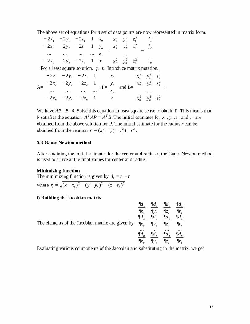
The above set of equations for n set of data points are now represented in matrix form.− − −− − −

− − −

−

+ ++ +

+ +

=

2 2 2 12 2 2 1

2 2 2 1

1 1 1

2 2 2

0 12

12

12

22

22

22

2 2 2

1

2

x y zx y z

x y z

xyz

x y zx y z

x y z

ff

fn n n

o

o

n n n n

... ... ... ... ...ρ

For a least square solution, f i =0. Introduce matrix notation,

A=

− − −− − −

− − −

2 2 2 12 2 2 1

2 2 2 1

1 1 1

2 2 2

x y zx y z

x y zn n n

... ... ... ..., P=

xyz

o

o

0

ρ

and B=

x y zx y z

x y zn n n

12

12

12

22

22

22

2 2 2

+ ++ +

+ +

...

.

We have AP - B=0. Solve this equation in least square sense to obtain P. This means thatP satisfies the equation A AP A BT T= .The initial estimates for xo , yo , zo and ρ areobtained from the above solution for P. The initial estimate for the radius r can beobtained from the relation ρ = + + −( )x y z ro o o

2 2 2 2 .

5.3 Gauss Newton method

After obtaining the initial estimates for the center and radius r, the Gauss Newton methodis used to arrive at the final values for center and radius.

Minimizing functionThe minimizing function is given by d r ri i= −where r x x y y z zi o o o= − + − + −( ) ( ) ( )2 2 2

i) Building the jacobian matrix

The elements of the Jacobian matrix are given by

∂∂

∂∂

∂∂

∂∂

∂∂

∂∂

∂∂

∂∂

∂∂

∂∂

∂∂

∂∂

dx

dy

dz

dr

dx

dy

dz

dr

dx

dy

dz

dr

o o o o

o o o o

n

o

n

o

n

o

n

o

1 1 1 1

2 2 2 2

... ... ... ...

Evaluating various components of the Jacobian and substituting in the matrix, we get

14

J

x xr

y yr

z zr

x xr

y yr

z zr

x xr

y yr

z zr

n

n

n

n

n

n

=

− − − − − −−

− − − − − −−

− − − − − −−

( ) ( ) ( )

( ) ( ) ( )

( ) ( ) ( )

1 0

1

1 0

1

1 0

1

2 0

2

2 0

21

2 0

2

0 0 0

1

1

1

ii) Solve the linear least square system J P = -d

where P

pppp

x

y

z

r

o

o

o

=

iii) Increment parameters according tox xo o= + pxo

;

y yo o= + pyo;

z zo o= + pzo;

r ro o= + pr ;

iv) Convergence conditionRepeat steps till algorithm has converged. The convergence condition is given byg J dT= is minimum.

6 Gauss-Newton Strategy for Cylinders

Any line can be specified by giving a point on the line and direction cosine(a,b,c). So it requires 6 numbers to describe a line. Its constraint is a2 + b2 + c2 =1. Sogiven two of components, the third can be determined. Consider a constraint on a linewhere c = 1, a vertical line, it is enough to specify two direction cosine a and b. Z can bedetermined from the relationship

ax+ by + cz = 0 (5.1)

Since c = 1, z = -ax -by (5.2)

So the advantage of this constraint is to minimize 6 parameters to 4 parameters a, b, x0,and y0. It also reduces the complication of solve Jacobean matrix and time to evaluatebecause the derivatives of distance is computed when using a Gauss-Newton method.

The Gauss-Newton algorithm is modified for the case of a cylinder. It is

15

1) Translate the coordinate system at beginning of each iteration, so the point on the axisis the origin of the coordinate system. It means that x = y =0.

2) Rotate the coordinate system so that the direction of the axis is along the z-axis. Soa=b=0 & c=1.

6.1 Rotational Concept

Figure 5.1 Example of how to develop rotational matrices

Consider a figure above, B={u1, u2, u3} is rotated to the new basis B'={u'1, u'2, u'3}, whereu1, u2, u3 and u'1, u'2, u'3 are unit vectors. u'1, u'2 , and u'3 can be expressed as

[ ]

=

0)sin()cos(

u B'1 θ

θ[ ]

=

0)cos()sin(-

u B'2 θ

θ[ ]

=

100

u B'3 (5.1.1)

So, the transition matrix from B' to B is

=

1000)cos()sin(0)sin(-)cos(

P θθθθ

(5.1.2)

and the transition matrix from B to B' is

=

1000)cos()sin(-0)sin()cos(

PT θθθθ

(5.1.3)

z z'

u3

u'3

u1

x x'

y'

y

θu'1

u2

u'2

16

So the new coordinates (x',y',z') can be computed from its old coordinates (x,y,z) by

=

zyx

1000)cos()sin(-0)sin()cos(

z'y'x'

θθθθ

(5.1.4)

7 Least Squares Best Fit Cylinders

Assume that a cylinder is fitted to m points (xi,yi, zi), where m ≥ 5

7.1 Parametrization

A cylinder can be specified by1) a point (x0, y0, z0) on its axis2) a vector (a,b,c) pointing a long the axis and3) its radius r

7.2 Initial estimate for a cylinder

Let a, b, c be the direction cosine of the axis. x0, y0 , and z0 are a point on the axis, and xi,yi, zi are any point on the cylinder. Then

A2 + B2 + C2 = R2 (6.2.1)

Where A = c( yi-y0 ) - b(zi - z0)B = a(zi - z0 ) - c(xi - x0)C = b(xi - x0) - a(yi - y0)R = initial estimate for radius.

Substitute into the equation above

[c( yi-y0 ) - b(zi - z0)]2 +[ a(zi - z0 ) - c(xi - x0)]2 + [b(xi - x0) - a(yi - y0)]2 = R2

This equation is simplified; it yields

Ax2 + By2 + Cz2 + Dxy + Exz + Fyz + Gx + Hy +Iz + J=0 (6.2.2)

Where A = (b2 + c2)B = (a2 + c2)C = (a2 + b2)D = -2abE = -2acF = -2bc

17

G = -2(b2 + c2)x0 + 2aby0 + 2acz0

H = 2abx0 - 2(a2 + c2)x0 + 2bcz0I = 2acx0 + 2bcy0 - 2(a2 + b2)z0

J = (b2 + c2) 20x + (a2 + c2) 2

0y + (a2 + b2) 20z - 2bcy0z0 - 2acz0x0 - 2abx0y0 - R2

Divide both sides by A

0AJz

AIy

AHx

AGyz

AFxz

AExy

ADz

ACy

AB x 222 =+++++++++

So

xAJz

AIy

AHx

AGyz

AFxz

AExy

ADz

ACy

AB 222 −=++++++++ (6.2.3)

This can be written as a linear system

−

=

2n

22

21

nnnnnnnnn2n

2n

22222222222

22

11111111121

21

x-

x-x

J/AI/AH/AG/AF/AE/AD/AC/AB/A

1zyxzyzxyxzy

1zyxzyzxyxy1zyxzyzxyxzy

MMMMMMMMMMz

(6.2.4)

This is the form of ATAP = ATB, and P can be solved as

P=(ATA)-1ATB (6.2.5)

Let C'=C/A, D'=D/A, E'=E/A, F'=F/A, G'=G/A, H'=H/A, I'=I/A, and J'=J/A.

Solving for this; if |D'|, |E'|, and |F'| are close to 0, then B' close to 1 implies (a b c) = (0 01), and C' close to 1 implies (a b c) =(0 1 0). Otherwise

)C'B'(12k++

= (6.2.6)

A =k, B=kB', C=kC', D=kD', E=kE', F=kF', G=kG', I=kI', and J=kJ' (6.2.7)

If A and B are close to 1c'=(1-C)1/2, a'=E/-2C', and b' = F/-2c'

If A is close to 1, B is not close to 1

18

b'=(1-B)1/2, a'=D/-2b', and c'=F/-2b'

If A is not close to 1a' = (1-A)1/2, b' = D/-2a', and c'=E/-2a'

The direction (a' b' c') is normalized to get the direction (a b c)

7.2.1 Initial estimate for the point on axis

Knowing ( a b c), the definition of the coefficients G, H, I and equation ax0 + by0+ cz0 = 0 are used to derive an estimate for (x0,y0,z0). These will form into the linearsystem as

=

+−+−

+−

0IHG

zyx

cba)ba(22bc2ac

2bc)ca(22ab2ac2ab)cb(2

0

0

0

22

22

22

(6.2.1.1)

This equation is solved by using the normal equation ATAP = ATB, where P contains theinitial estimate for the point in the axis.

7.2.2 Initial Estimate for radius This can be done by using the definition of J that is

J = (b2 + c2) 20x + (a2 + c2) 2

0y + (a2 + b2) 20z - 2bcy0z0 - 2acz0x0 - 2abx0y0 - R2

SoR2 = (b2 + c2) 2

0x + (a2 + c2) 20y + (a2 + b2) 2

0z - 2bcy0z0 - 2acz0x0 - 2abx0y0 – J (6.2.2.1)

7.3 Algorithm description1. Translate of the origin

Translate (a copy of) the data so that the point on the axis lies at centroid of the point

)z,y,(x- )z,y,x( )z,y,x( ccciiiiii = (6.3.1)

2. Transform the data by a rotation matrix U which rotates (a b c) to a point the z-axis

=

i

i

i

i

i

i

zyx

Uzyx

(6.3.2)

where U is

19

=

11

11

22

22

cs-0sc0001

c0c-010s0c

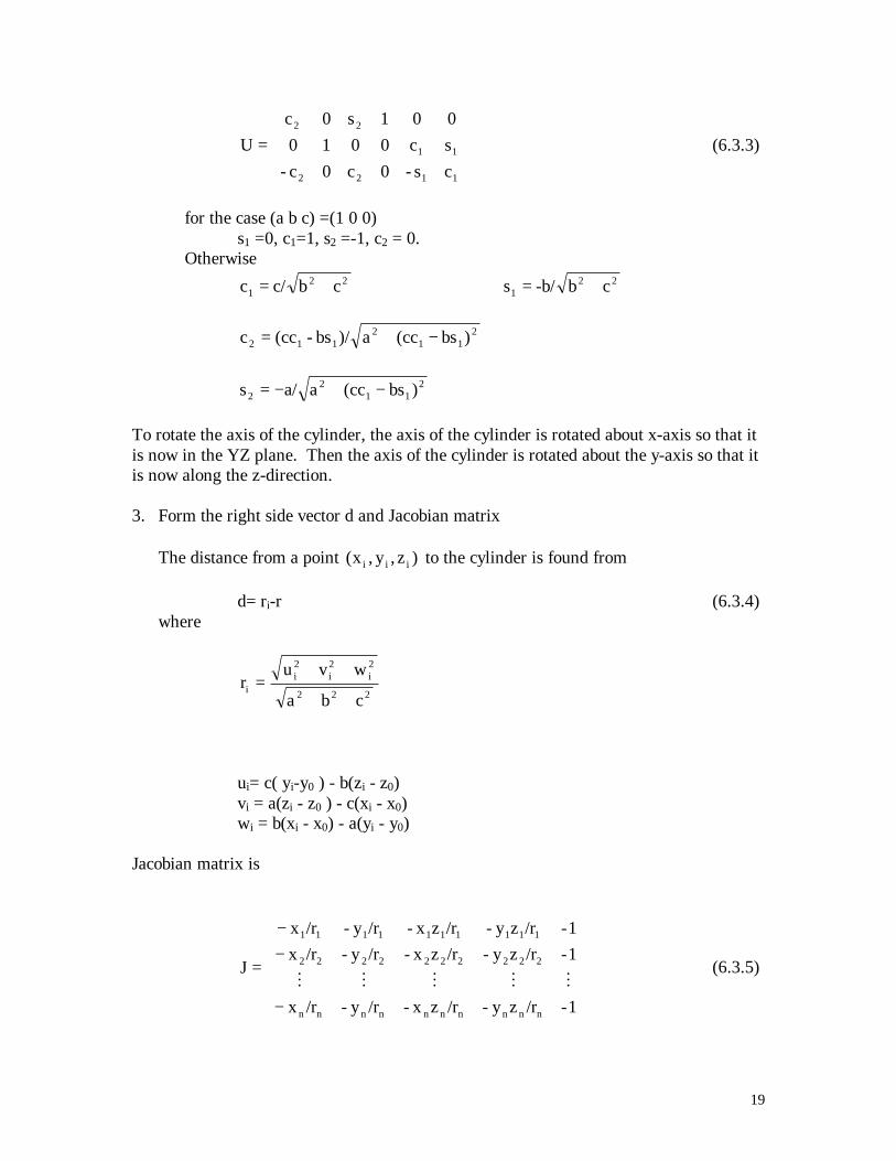
U (6.3.3)

for the case (a b c) =(1 0 0)s1 =0, c1=1, s2 =-1, c2 = 0.

Otherwise22

1 cbc/c += 221 cb-b/s +=

211

2112 )bscc(a)/bs-cc(c −+=

211

22 )bscc(aa/s −+−=

To rotate the axis of the cylinder, the axis of the cylinder is rotated about x-axis so that itis now in the YZ plane. Then the axis of the cylinder is rotated about the y-axis so that itis now along the z-direction.

3. Form the right side vector d and Jacobian matrix

The distance from a point )z,y,x( iii to the cylinder is found from

d= ri-r (6.3.4)where

222

2i

2i

2i

icba

wvur

++++

=

ui= c( yi-y0 ) - b(zi - z0)vi = a(zi - z0 ) - c(xi - x0)wi = b(xi - x0) - a(yi - y0)

Jacobian matrix is

−

−−

=

1-/rzy-/rzx-/ry-/rx

1-/rzy-/rzx-/ry-/rx1-/rzy-/rzx-/ry-/rx

J

nnnnnnnnnn

2222222222

1111111111

MMMMM(6.3.5)

20

4. Solve the linear least-squares system

d

ppppp

J

r

b

a

y0

x0

−=

(6.3.6)

5. update the parameter estimates according to

+

=

by0ax0

y0

x0T

0

0

0

0

0

0

pp-pp-pp

Uzyx

zyx

(6.3.7)

=

1pp

Ucba

b

aT (6.3.8)

r = r + pr (6.3.9)

Steps above are repeated until the algorithm has converged. In step I, (a copy of) theoriginal data set is used rather than a transformed set from a previous iteration.

6. If we want to present (x0, y0, z0) on the line nearest the origin, then

++++−

=

cb

zz

a

cbaczbyax

yx

yx

222000

0

0

0

0

0

0

(6.3.10)

8 Conclusion

In this report, the least square fitting algorithms for lines, planes, circles, spheresand cylinders were discussed in detail. They the implementation of the algorithm usingMATLAB and the source code is included in the appendix. The mathematical stepsinvolved in the implementation are also discussed in detail. The summaries of the articlesthat were used as reference for doing this project were also included as appendix.

21

9 References

1. Forbes, Alistair B., Least Squares Best-Fit geometric elements, NPL report April1989.

2. Assessment of Position, size and departure from nominal form of geometric features,British Standards Institution, BS7172: 1989

3. Computational Metrology, Manufacturing Review, Vol 6, No 4,19934. Press, William H. Flannery, Brian P, Teukolsy, Saul A, Vetterling, William T.,

Numerical Recipes in C, The aart of Scientific computing, Cambridge universityPress.

5. Ramakrishna Machireddy, Sampling techniques for plane geometry for coordiantemeasuring machines, MS Thesis, UNCC 1992

6. Uppliappan Babu, Sampling Methods and substitute Geometry for Measuringcylinders in a Co-ordiante Measuring Machines(Chapter 2), MS Thesis ,UNCC 1993

7. Anton Rorres, Element Linear Algebra Application Version, NY 1991.

22