1.1 an introduction to limits1.1 an introduction to limits estimating limits numerically example...
TRANSCRIPT
1.1 An introduction to limits
Definition(Informal definition)If we can make the values of a function f (x) get arbitrarily close to anumber L by taking x-values that are sufficiently close to c (but notequal to c), then we say the limit of f (x) as x approaches c is L, and wewrite
limx→c
f (x) = L
RemarkWe need to define more clearly what is means to be arbitrarily closeand sufficiently close in order to make the informal definition of limitgiven above more rigorous. We’ll do that in the next section. For now,we’ll use this informal definition to explore the idea of a limit byestimating limits (a) graphically and (b) numerically.
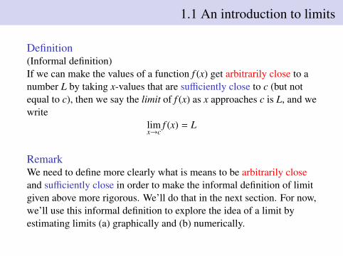
1.1 An introduction to limits
Estimating limits graphically
Example
Find
• limx→5
√3x + 1 =
• limx→1
√3x + 1 =
• limx→0
√3x + 1 =
• limx→8
√3x + 1 =
• limx→2
√3x + 1 =
y =√
3x + 1

1.1 An introduction to limits
y =√
3x + 1

1.1 An introduction to limits
Estimating limits graphically
Example
Find
• limx→5
√3x + 1 = 4
• limx→1
√3x + 1 = 2
• limx→0
√3x + 1 = 1
• limx→8
√3x + 1 = 5
• limx→2
√3x + 1 ≈ 2.7
y =√
3x + 1

1.1 An introduction to limits
Estimating limits numerically
Example
Find limx→3
2x2 − 2x − 12x − 3
SolutionPick x-values near 3 (but not equal to 3) and compute the value of thefunction.
x 2x2−2x−12x−3 x 2x2−2x−12
x−32.9 3.12.99 3.012.999 3.001
How close to 3 would x have to be in order to get within• 0.0002 of the limit?• 0.1 of the limit?

1.1 An introduction to limits
Estimating limits numerically
Example
Find limx→3
2x2 − 2x − 12x − 3
SolutionPick x-values near 3 (but not equal to 3) and compute the value of thefunction.
x 2x2−2x−12x−3 x 2x2−2x−12
x−32.9 9.8 3.1 10.22.99 9.98 3.01 10.022.999 9.998 3.001 10.002
How close to 3 would x have to be in order to get within• 0.0002 of the limit? (within 0.0001 of 3)• 0.1 of the limit? (within 0.05 of 3)

1.1 An introduction to limits
When limits do not exist
RemarkA function may not have a limit for all values of x. There are threeways a limit may fail to exist as x approaches c:
1 The function may approach different values on either side of c orfail to exist near c.
2 The function may grow without bound (i.e. tend toward +∞ or−∞) as x approaches c.
3 The function may oscillate infinitely often as x approaches cwithout staying near any single value.
In the following slides we give examples of each case.
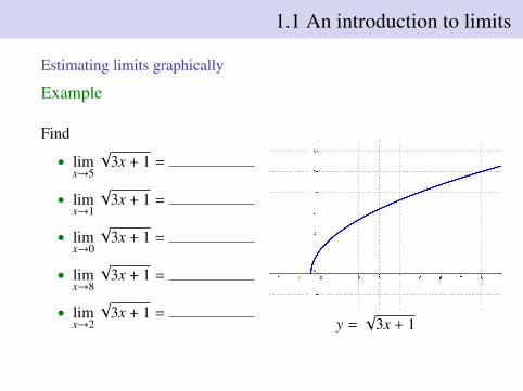
1.1 An introduction to limits
When limits do not exist: (1) different values from left and right
Example
Consider
f (x) =|x|x
=
{ xx = 1 x > 0−xx = −1 x < 0
y = |x|/x
limx→0
|x|x
does not exist because limx→0+
|x|x
= 1 (the right-hand limit) while
limx→0−
|x|x
= −1 (the left-hand limit).
1.1 An introduction to limits
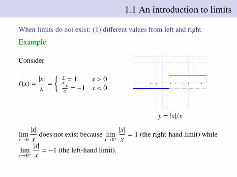
When limits do not exist: (1) function fails to exist near c
Example
Consider
f (x) =√
3x + 1
y =√
3x + 1
limx→−1/3
√3x + 1 does not exist because f (x) =
√3x + 1 does not exist
for x < −1/3.

1.1 An introduction to limits
When limits do not exist: (2) function grows without bound
Example
Consider
f (x) =1
(x − 2)2
y = 1/(x − 2)2
limx→2
1/(x − 2)2 does not exist because there is no number L that the
function 1/(x − 2)2 gets closer to as x approaches 2; indeed, the valuesof the function 1/(x − 2)2 can be made as large as we’d like by takingx sufficiently close to 2. In other words, the function grows withoutbound as x approaches 2.

1.1 An introduction to limits
When limits do not exist: (3) function oscillates without staying neara single value
Example
Consider
f (x) = sin(1/x)
y = sin(1/x)
limx→0
sin(1/x) does not exist because there is no number L that the
function sin(1/x) gets closer to as x approaches 0; indeed, the valuesof the function sin(1/x) oscillate more rapidly between −1 and 1 as xapproaches 0.
1.1 An introduction to limits
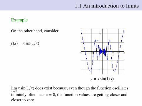
Example
On the other hand, consider
f (x) = x sin(1/x)
y = x sin(1/x)
limx→0
x sin(1/x) does exist because, even though the function oscillates
infinitely often near x = 0, the function values are getting closer andcloser to zero.
1.1 An introduction to limits
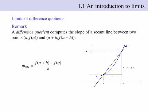
Limits of difference quotients
RemarkA difference quotient computes the slope of a secant line between twopoints (a, f (a)) and (a + h, f (a + h)):
msec =f (a + h) − f (a)
h

1.1 An introduction to limits
Limits of difference quotients
RemarkTaking the limit of these difference quotients as h→ 0 will give us theslope of the line that is tangent to y = f (x) at the point (a, f (a)):
mtan = limh→0
f (a + h) − f (a)h
Link: GeoGebra tangent line slope.ggb

1.1 An introduction to limits
Just checking. . . .1 True or false: The limit of f (x) as x approaches 5 is f (5).2 Approximate lim
x→0f (x) numerically and graphically, where
f (x) =
{cos x x ≤ 0x2 + 3x + 1 x > 0
}, or state why the limit does not
exist.
3 Approximate limx→2
x2 + 7x + 10x2 − 4x + 4
numerically and graphically, or
state why the limit does not exist.4 Approximate lim
x→2f (x) numerically and graphically, where
f (x) =
{x + 1 x < 23x − 5 x ≥ 2
}, or state why the limit does not exist.
5 Consider the function f (x) = ln x and the point a = 5.
Approximate the limit of the difference quotientf (a + h) − f (a)
hby using h = ±0.1,±0.01.

1.2 Epsilon-delta definition of a limit
Toward a more rigorous definition
Definition(Informal definitions) Given a function y = f (x) and an x-value c, wesay that lim
x→cf (x) = L provided
1 y = f (x) is near L whenever x is near c.
2 whenever x is within a certain tolerance level of c, then thecorresponding value y = f (x) is within a certain tolerance level ofL.
RemarkThe tolerances for x and y are different. The y-tolerance is called ε,and the x-tolerance is called δ.

1.2 Epsilon-delta definition of a limit
A rigorous definition of limit
Definition(Rigorous definition) Let f be a function defined on an open intervalcontaining c. Then lim
x→cf (x) = L provided that given any ε > 0, there
exists a corresponding δ > 0 such that whenever 0 < |x − c| < δ, wehave |f (x) − L| < ε.

1.2 Epsilon-delta definition of a limit
Examples
Example
1 Show limx→9
√x = 3. (Cf. §1.2: Example 6)
2 Show limx→4
x2 = 16. (Cf. §1.2: Example 7)
3 Show limx→0
ex = 1. (Cf. §1.2: Example 8)
4 Show limx→c
ex = ec.
RemarkThis last example show that the function f (x) = ex is continuous at allvalues of x. More generally, a function f (x) is continuous at c iflimx→c
f (x) = f (c). We’ll explore this important idea of continuity morein §1.5.

1.2 Epsilon-delta definition of a limit
Just checking. . . .1 What’s wrong with the following “definition” of a limit?
The limit of f (x) as x approaches a is K means that given anyδ > 0, there exists an ε > 0 such that whenever |f (x) − K| < ε wehave 0 < |x − c| < δ.
2 Using an ε − δ argument, show limx→3
5 = 5.
3 Using an ε − δ argument, show limx→2
3 − 2x = −1.
4 Using an ε − δ argument, show limx→3
x2 − 3 = 6.
5 Using an ε − δ argument, show limx→0
e2x − 1 = 0.

1.3 Finding limits analytically
Limit Laws
TheoremLet b, c,L and K be real numbers, let n be a positive integer, and let fand g be functions with the following limits:
limx→c
f (x) = L limx→c
g(x) = K
Then the following limits hold:
1 limx→c
b = b
2 limx→c
x = c
3 limx→c
[f (x) ± g(x)] = L ± K
4 limx→c
b · f (x) = bL
5 limx→c
f (x) · g(x) = LK
6 limx→c
f (x)/g(x) = L/K(K , 0)
7 limx→c
[f (x)]n = Ln
8 limx→c
n√
f (x) =n√L
9 And if limx→c
f (x) = L andlimx→L
g(x) = K, then
limx→c
g(f (x)) = K.

1.3 Finding limits analytically
Using Limit Laws
ExampleSuppose lim
x→2f (x) = 3 and lim
x→2g(x) = −2 and p(x) = x2 − 3x + 1. Find:
1 limx→2
f (x) + g(x) =
2 limx→2
[g(x)]3 =
3 limx→2
p(x) =
4 limx→2
f (x) − 3p(x) =

1.3 Finding limits analytically
Using Limit Laws
ExampleSuppose lim
x→2f (x) = 3 and lim
x→2g(x) = −2 and p(x) = x2 − 3x + 1. Find:
1 limx→2
f (x) + g(x) = 1
2 limx→2
[g(x)]3 = −8
3 limx→2
p(x) = −1
4 limx→2
f (x) − 3p(x) = 6
RemarkNotice that
limx→2
p(x) = −1 = p(2)
Whenever limx→c
f (x) = f (c), we say that f is continuous at c. We willstudy continuity in greater detail in §1.5.
1.3 Finding limits analytically
Other Limit Laws
TheoremLet p(x) and q(x) be polynomials and c a real number. Then:
1 limx→c
p(x) = p(c)
2 limx→c
p(x)q(x)
=p(c)q(c)
, where q(c) , 0
RemarkSo polynomials are continuous everywhere and rational functions arecontinuous at every point in their domain. The next theorem listsother common continuous functions.

1.3 Finding limits analytically
Other Limit Laws
TheoremLet c be a real number in the domain of the given function, let n be apositive integer, and let a > 0. Then the following limits hold:
1 limx→c
sin x = sin c
2 limx→c
cos x = cos c
3 limx→c
tan x = tan c
4 limx→c
csc x = csc c
5 limx→c
sec x = sec c
6 limx→c
cot x = cot c
7 limx→c
ax = ac
8 limx→c
ln x = ln c
9 limx→c
n√x =n√c
ExampleEvaluate the following limits:
1 limx→π/3
cos x =
2 limx→3
csc2 x − cot2 x =
3 limx→0
ln e3x =
4 limx→1
e√
4x =

1.3 Finding limits analytically
Other Limit Laws
TheoremLet c be a real number in the domain of the given function, let n be apositive integer, and let a > 0. Then the following limits hold:
1 limx→c
sin x = sin c
2 limx→c
cos x = cos c
3 limx→c
tan x = tan c
4 limx→c
csc x = csc c
5 limx→c
sec x = sec c
6 limx→c
cot x = cot c
7 limx→c
ax = ac
8 limx→c
ln x = ln c
9 limx→c
n√x =n√c
ExampleEvaluate the following limits:
1 limx→π/3
cos x = 1/2
2 limx→3
csc2 x − cot2 x = 1
3 limx→0
ln e3x = 0
4 limx→1
e√
4x = e2

1.3 Finding limits analytically
Squeeze theorem
Theorem(Squeeze theorem) Let f , g and h be functions on an open interval Icontaining c such that for all x in I we have f (x) ≤ g(x) ≤ h(x). If
limx→c
f (x) = L = limx→c
h(x)
thenlimx→c
g(x) = L
Example
(A fundamental trig limit) limx→0
sin xx
= 1
RemarkThis says that sin x and x are approaching 0 at the same rate.

1.3 Finding limits analytically
Special limits
Theorem
1 limx→0
sin xx
= 1
2 limx→0
cos x − 1x
= 0
3 limx→0
(1 + x)1/x = e
4 limx→0
ex − 1x
= 1
RemarkSo, cos x − 1 approaches 0 faster than x does, while ex − 1 and xapproach 0 at the same rate. These are all examples of indeterminateforms, which we will study in more detail in a later section (§6.7).
1.3 Finding limits analytically
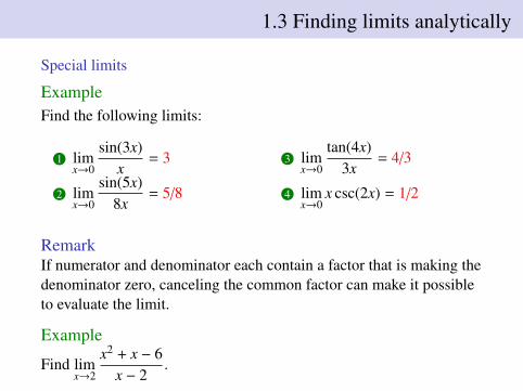
Special limits
ExampleFind the following limits:
1 limx→0
sin(3x)x
=
2 limx→0
sin(5x)8x
=
3 limx→0
tan(4x)3x
=
4 limx→0
x csc(2x) =
RemarkIf numerator and denominator each contain a factor that is making thedenominator zero, canceling the common factor can make it possibleto evaluate the limit.
Example
Find limx→2
x2 + x − 6x − 2
.
1.3 Finding limits analytically
Special limits
ExampleFind the following limits:
1 limx→0
sin(3x)x
= 3
2 limx→0
sin(5x)8x
= 5/8
3 limx→0
tan(4x)3x
= 4/3
4 limx→0
x csc(2x) = 1/2
RemarkIf numerator and denominator each contain a factor that is making thedenominator zero, canceling the common factor can make it possibleto evaluate the limit.
Example
Find limx→2
x2 + x − 6x − 2
.

1.3 Finding limits analytically
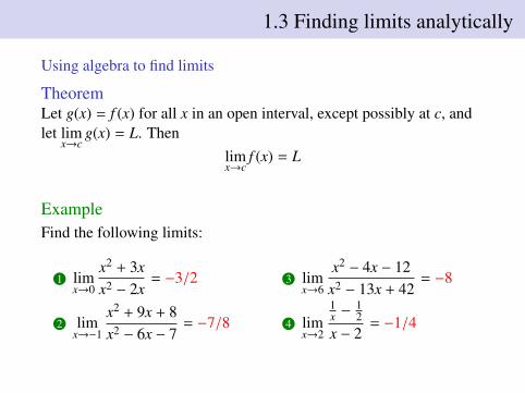
Using algebra to find limits
TheoremLet g(x) = f (x) for all x in an open interval, except possibly at c, andlet lim
x→cg(x) = L. Then
limx→c
f (x) = L
ExampleFind the following limits:
1 limx→0
x2 + 3xx2 − 2x
=
2 limx→−1
x2 + 9x + 8x2 − 6x − 7
=
3 limx→6
x2 − 4x − 12x2 − 13x + 42
=
4 limx→2
1x −
12
x − 2=
1.3 Finding limits analytically
Using algebra to find limits
TheoremLet g(x) = f (x) for all x in an open interval, except possibly at c, andlet lim
x→cg(x) = L. Then
limx→c
f (x) = L
ExampleFind the following limits:
1 limx→0
x2 + 3xx2 − 2x
= −3/2
2 limx→−1
x2 + 9x + 8x2 − 6x − 7
= −7/8
3 limx→6
x2 − 4x − 12x2 − 13x + 42
= −8
4 limx→2
1x −
12
x − 2= −1/4

1.3 Finding limits analytically
Just checking. . . .1 You are given the following information:
• limx→1
f (x) = 0 = limx→1
g(x)• lim
x→1f (x)/g(x) = 2.
What can be said about the relative sizes of f (x) and g(x) as xapproaches 1?
2 Find limx→0
5xcos(3x)
.
3 Find limx→0
5xsin(3x)
.
4 Find limx→π/4
cos x sin x.
5 Find limx→−2
x2 − 5x − 14x2 + 10x + 16
.

1.4 One-sided limits
Left- and right-hand limits
DefinitionLet f be a function defined on an open interval containing c. Thenotation
limx→c−
f (x) = L,
which is read as “the limit of f (x) as x approaches c from the left is L,”or “the left-hand limit of f at c is L,” means that:
given any ε > 0, there exists δ > 0 such that whenever0 < c − x < δ, we have |f (x) − L| < ε.
RemarkWhat changes need to be made to define a right-hand limit at c?
1.4 One-sided limits
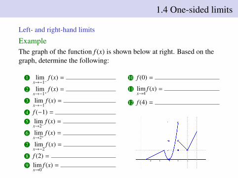
Left- and right-hand limits
ExampleThe graph of the function f (x) is shown below at right. Based on thegraph, determine the following:
1 limx→−1−
f (x) =
2 limx→−1+
f (x) =
3 limx→−1
f (x) =
4 f (−1) =
5 limx→2−
f (x) =
6 limx→2+
f (x) =
7 limx→−2
f (x) =
8 f (2) =
9 limx→0
f (x) =
10 f (0) =
11 limx→4
f (x) =
12 f (4) =

1.4 One-sided limits
Left- and right-hand limits
ExampleThe graph of the function f (x) is shown below at right. Based on thegraph, determine the following:
1 limx→−1−
f (x) = 2
2 limx→−1+
f (x) = 2
3 limx→−1
f (x) = 2
4 f (−1) = 25 lim
x→2−f (x) = 8
6 limx→2+
f (x) = 4
7 limx→−2
f (x) = dne
8 f (2) = 29 lim
x→0f (x) = 0
10 f (0) = 4
11 limx→4
f (x) = 2
12 f (4) = dne

1.4 One-sided limits
Left- and right-hand limits
RemarkFrom this example, we learn two important things about limits. First,limx→c
f (x) and f (c) are independent of one another:
limx→c
f (x) can be f (c), but it need not be; in fact, limx→c
f (x) can existeven if f (c) doesn’t exist, and vice versa.
The second important thing we learn from this example is . . .
TheoremLet f be a function defined on an open interval I containing c. Then
limx→c
f (x) = L ⇐⇒ limx→c−
f (x) = L and limx→c+
f (x) = L

1.4 One-sided limits
Just checking. . . .
1 True or false: if limx→5−
f (x) = 3, then limx→5
f (x) = 3.
2 True or false: if limx→5
f (x) = 3, then limx→5−
f (x) = 3.
3 True or false: if limx→5
f (x) = 3, then f (5) = 3.
4 Estimate the limit numerically: limx→0.2
x2 + 5.8x − 1.2x2 − 4.2x + 0.8
5 Evaluate the limit: limx→3
x2 − 6x + 9x3 − 3x

1.5 Continuity
DefinitionLet f be a function defined on an open interval I containing c.
1 f is continuous at c if limx→c
f (x) = f (c).
2 f is continuous on I if f is continuous at c for all values of c in I.If f is continuous on (−∞,∞), we say f is continuouseverywhere.
DefinitionLet f be defined on the closed interval [a, b] for some real numbersa, b. f is continuous on [a, b] if:
1 f is continuous on (a, b),
2 limx→a+
f (x) = f (a), and
3 limx→b−
f (x) = f (b).

1.5 Continuity
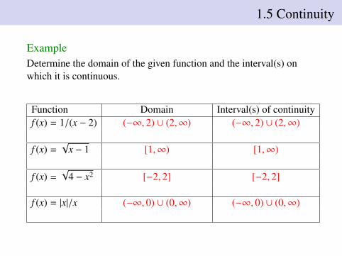
ExampleDetermine the domain of the given function and the interval(s) onwhich it is continuous.
Function Domain Interval(s) of continuityf (x) = 1/(x − 2)
f (x) =√
x − 1
f (x) =√
4 − x2
f (x) = |x|/x
1.5 Continuity
ExampleDetermine the domain of the given function and the interval(s) onwhich it is continuous.
Function Domain Interval(s) of continuityf (x) = 1/(x − 2) (−∞, 2) ∪ (2,∞) (−∞, 2) ∪ (2,∞)
f (x) =√
x − 1 [1,∞) [1,∞)
f (x) =√
4 − x2 [−2, 2] [−2, 2]
f (x) = |x|/x (−∞, 0) ∪ (0,∞) (−∞, 0) ∪ (0,∞)

1.5 Continuity
Properties of continuous functions
TheoremLet f and g be continuous functions on an interval I, let c be a realnumber, and let n be a positive integer. The following functions arecontinuous on I.
1 f ± g
2 c · f
3 f · g
4 f /g (g , 0 on I)
5 f n
6n√
f
7 If the range of f is J and g is continuous on J, then g ◦ f iscontinuous on I.

1.5 Continuity
Common continuous functions
TheoremThe following functions are continuous on their domains.
1 f (x) = sin x
2 f (x) = cos x
3 f (x) = tan x
4 f (x) = csc x
5 f (x) = sec x
6 f (x) = cot x
7 f (x) = ln x
8 f (x) = ax (a > 0)
9 f (x) = n√x(n a positive integer)
ExampleFind the interval(s) on which the following functions are continuous.
1 f (x) =√
3 − x +√
2x − 1 is continuous on
2 f (x) =√
ln(2x + 3) is continuous on
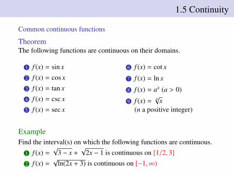
1.5 Continuity
Common continuous functions
TheoremThe following functions are continuous on their domains.
1 f (x) = sin x
2 f (x) = cos x
3 f (x) = tan x
4 f (x) = csc x
5 f (x) = sec x
6 f (x) = cot x
7 f (x) = ln x
8 f (x) = ax (a > 0)
9 f (x) = n√x(n a positive integer)
ExampleFind the interval(s) on which the following functions are continuous.
1 f (x) =√
3 − x +√
2x − 1 is continuous on [1/2, 3]
2 f (x) =√
ln(2x + 3) is continuous on [−1,∞)

1.5 Continuity
Intermediate value theorem
Theorem(Intermediate value theorem) Let f be a continuous function on [a, b].Then for every value y-value in between f (a) and f (b), there is anx-value c in [a, b] such that f (c) = y.
RemarkThe IVT is an existence theorem: it asserts the existence of an x-valuec with f (c) = y for every y in between f (a) and f (b). We can find agood approximation of c using the bisection method, as illustrated inthe next example.

1.5 Continuity
Example(Bisection method) Find the root of f (x) = x3 + x + 1 accurate to twodecimal places.
Iteration Interval Midpoint sign1 [−1, 0] f (−0.5) > 02 [−1,−0.5] f (−0.75) < 03 [−0.75,−0.5] f (−0.625) > 04 [−0.75,−0.625] f (−0.6875) < 05 [−0.6875,−0.625] f (−0.65625) > 06 [−0.6875,−0.65625] f (−0.67188) > 07 [−0.6875,−0.67188] f (−0.67969) > 08 [−0.6875,−0.67969] f (−0.68359) < 09 [−0.68359,−0.67969]

1.5 Continuity
Just checking. . . .
1 True or false: If f is defined on an open interval containing c andlimx→c
f (x) exists, then f is continuous at c.
2 True or false: If f is continuous at c, then limx→c
f (x) exists.
3 True or false: If f is continuous at c, then limx→c
f (x) = f (c).
4 True or false: If f is continuous on [0, 1) and on [1, 2], then f iscontinuous on [0, 2].
5 Let f (x) =
{x2 x ≤ 23 − mx x > 2
}. Find the value of m that makes f
continuous at x = 2.

1.6 Limits involving infinity
Infinite limits
DefinitionWe say lim
x→cf (x) = ∞ if for every M > 0 there exists δ > 0 such that if
0 < |x − c| < δ, then f (x) ≥ M
Example
1 limx→3
1(x − 3)2 = ∞
2 limx→π/2−
tan x = ∞ and limx→π/2+
tan x = −∞.
DefinitionIf the limit of f (x) as x approaches c from either the right or the left(or both) is∞ or −∞, we say that the function has a verticalasymptote at c.

1.6 Limits involving infinity
Infinite limits
Example
1 f (x) =x2
x2 − 1has vertical asymptotes at x = 1 and x = −1.
2 f (x) =x3 + 2x2 − x − 2
x2 − 1does not. Indeed, f (x) = x + 2 for all x
except x = 1 and x = −1, where is simply has a hole (i.e. pointdiscontinuity).
RemarkThe above example illustrates the fact that just because a function hasa denominator of zero for particular values of x does not mean that ithas a vertical asymptote at those values of x. It must also have aninfinite limit (from the left, or from the right, or both) in order to havea vertical asymptote.

1.6 Limits involving infinity
Limits at infinity
Definition
1 We say that limx→∞
f (x) = L if for every ε > 0 there exists M > 0such that if x ≥ M, then |f (x) − L| < ε.
2 We say that limx→−∞
f (x) = L if for every ε > 0 there exists M < 0such that if x ≤ M, then |f (x) − L| < ε.
3 If limx→∞
f (x) = L or limx→−∞
f (x) = L, we say that y = L is ahorizontal asymptote of f .
ExampleFind the horizontal asymptote(s) of the following functions.
1 f (x) =x2
x2 − 12 f (x) =
3x√
x2 + 13 f (x) =
sin xx

1.6 Limits involving infinity
Limits at infinity
Definition
1 We say that limx→∞
f (x) = L if for every ε > 0 there exists M > 0such that if x ≥ M, then |f (x) − L| < ε.
2 We say that limx→−∞
f (x) = L if for every ε > 0 there exists M < 0such that if x ≤ M, then |f (x) − L| < ε.
3 If limx→∞
f (x) = L or limx→−∞
f (x) = L, we say that y = L is ahorizontal asymptote of f .
ExampleFind the horizontal asymptote(s) of the following functions.
1 f (x) =x2
x2 − 1y = 1
2 f (x) =3x
√x2 + 1
y = ±3
3 f (x) =sin x
xy = 0

1.6 Limits involving infinity
Limits at infinity
TheoremSuppose we have a rational function
f (x) =anxn + · · · + a1x + a0
bmxm + · · · + b1x + b0
where any of the coefficients may be zero except for an and bm.
1 If n = m, then limx→±∞
f (x) =an
bm2 If n < m, then lim
x→±∞f (x) = 0.
3 If n > m, then limx→∞
f (x) and limx→−∞
f (x) are both infinite.

1.6 Limits involving infinity
Limits at infinity
ExampleFind the following limits.
1 limx→∞
6x − 2x2
x2 − 2x − 3=
2 limx→−∞
6x − 2x3
x2 − 2x − 3=
3 limx→∞
6x − 2x2
x3 − 2x − 3=
4 limx→3
6x − 2x2
x2 − 2x − 3=

1.6 Limits involving infinity
Limits at infinity
ExampleFind the following limits.
1 limx→∞
6x − 2x2
x2 − 2x − 3= −2
2 limx→−∞
6x − 2x3
x2 − 2x − 3=∞
3 limx→∞
6x − 2x2
x3 − 2x − 3= 0
4 limx→3
6x − 2x2
x2 − 2x − 3= −3/2

1.6 Limits involving infinity
Just checking. . . .
1 True or false: If limx→3
f (x) = ∞, then f has a vertical asymptote at
x = 3.
2 True or false: If limx→3
f (x) = ∞, then f (3) is not defined at x = 3.
3 True or false: If limx→3
f (x) = ∞, then f is not continuous at x = 3.
4 Using a ε − δ argument, show that limx→1
3x − 1 = 2.
5 Evaluate the limit limx→−4
x2 − 16x2 − 4x − 32
.