11 20968 kathirvel r 3d based remote sensing image ... · the ground surface area that forms one...

Journal of Theoretical and Applied Information Technology 31

st March 2014. Vol. 61 No.3

© 2005 - 2014 JATIT & LLS. All rights reserved.

ISSN: 1992-8645 www.jatit.org E-ISSN: 1817-3195

545

3D BASED REMOTE SENSING IMAGE CONTRAST

ENHANCEMENT USING SVM

R.KATHIRVEL, DR.J.SUNDARARAJAN

ABSTRACT

A satellite image is full of noisy information thus it faces many problems just to get a clear view of a location. Various image enhancement techniques are used to remove the unwanted data from the satellite image. Existing techniques fail to clear noise from the satellite image enough to be used for real time purposes. To overcome this problem we propose SVM which has two significant parts. The first one is the interior point method and second one is boundary value selection. The majority of color histogram equalization methods do not yield uniform histogram in gray scale. Contrast of the converted image is worse in 1D and 2D, to overcome this we move on to 3D. The new satellite image contrast enhancement technique is based on the discrete wavelet transform (DWT) which decomposes the input image into the four frequency sub bands by using DWT and estimates the singular value matrix of the low- low sub band image, and, then, it reconstructs the enhanced image by applying inverse DWT.

Keywords: Support Vector Machine, Interior Point Method, Boundary Value Selection, DWT With 3D.

1. INTRODUCTION

1.1. Support vector machines

Support Vector Machines are based on the concept of decision planes that define decision boundaries. A decision plane is one that separates between a set of objects having different class memberships. A schematic example is shown in the illustration below. In this example, the objects belong either to class GREEN or RED. The separating line defines a boundary on the right side of which all objects are GREEN and to the left of which all objects are RED. Any new object (white circle) falling to the right is labeled, i.e., classified, as GREEN (or classified as RED should it fall to the left of the separating line).

The above is a classic example of a linear classifier, i.e., a classifier that separates a set of objects into their respective groups (GREEN and RED in this case) with a line. Most classification tasks, however, are not that simple, and often more complex structures are needed in order to make an optimal separation, i.e., correctly classify new

objects (test cases) on the basis of the examples that are available (train cases). This situation is depicted in the illustration below. Compared to the previous schematic, it is clear that a full separation of the GREEN and RED objects would require a curve (which is more complex than a line). Classification tasks based on drawing separating lines to distinguish between objects of different class memberships are known as hyperplane classifiers. Support Vector Machines are particularly suited to handle such tasks.

The illustration below shows the basic idea behind Support Vector Machines. Here we see the original objects (left side of the schematic) mapped, i.e., rearranged, using a set of mathematical functions, known as kernels. The process of rearranging the objects is known as mapping (transformation). Note that in this new setting, the mapped objects (right side of the schematic) is linearly separable and, thus, instead of constructing the complex curve (left schematic), all we have to do is to find an optimal line that can separate the GREEN and the RED objects.





546

The science of acquiring information about an object, without entering in contact with it, by sensing and recording reflected or emitted energy and processing, analyzing, and applying that information. Remote sensing can be broadly defined as the collection and interpretation of information about an object, area, or even without being in physical contact with the object. Aircraft and satellites are the common platforms for remote sensing of the earth and its natural resources. Aerial photography in the visible portion of the electromagnetic wavelength was the original form of remote sensing but technological developments has enabled the acquisition of information at other wavelengths including near infrared, thermal infrared and microwave. Collection of information over a large numbers of wavelength bands is referred to as multispectral or hyper spectral data. The development and deployment of manned and unmanned satellites has enhanced the collection of remotely sensed data and offers an inexpensive way to obtain information over large areas. The capacity of remote sensing to identify and monitor land surfaces and environmental conditions has expanded greatly over the last few years and remotely sensed data will be an essential tool in natural resource management. 1.2. Satellite sensor characteristics

The basic functions of most satellite sensors are to collect information about the reflected radiation along a pathway, also known as the field of view (FOV), as the satellite orbits the Earth. The smallest area of ground that is sampled is called the instantaneous field of view (IFOV). The IFOV is also described as the pixel size of the sensor. This sampling or measurement occurs in one or many spectral bands of the EM spectrum. The data collected by each satellite sensor can be described in terms of spatial, spectral and temporal resolution. 1.3. Passive sensors

Detect natural radiation that is emitted or

reflected by the object being observed. Sunlight is the most common source of radiation. 1.4. Active sensors

Emit energy in order to scan objects and areas. The time delay between emission and return is measured, establishing the location, height, speed and direction of an object. 1.5. Spatial resolution

The spatial resolution (also known as ground resolution) is the ground area imaged for the instantaneous field of view (IFOV) of the sensing device. Spatial resolution may also be described as the ground surface area that forms one pixel in the satellite image. The IFOV or ground resolution of the Landsat Thematic Mapper (TM) sensor, for example, is 30 m. The ground resolution of weather satellite sensors is often larger than a square kilo meter. There are satellites that collect data at less than one meter ground resolution but these are classified military satellites or very expensive commercial systems. 1.6. Temporal resolution

Temporal resolution is a measure of the repeat cycle or frequency with which a sensor revisits the same part of the Earth’s surface. The frequency will vary from several times per day, for a typical weather satellite, to 8—20 times a year for a moderate ground resolution satellite, such as Landsat TM. The frequency characteristics will be determined by the design of the satellite sensor and its orbit pattern 1.7. Spectral resolution

The spectral resolution of a sensor system is the number and width of spectral bands in the sensing device. The simplest form of spectral resolution is a sensor with one band only, which senses visible light. An image from this sensor would be similar in appearance to a black and white photograph from an aircraft. A sensor with three spectral bands in the visible region of the EM spectrum would collect similar information to that of the human vision system. The Landsat TM sensor has seven spectral bands located in the visible and near to mid infrared parts of the spectrum. A panchromatic image consists of only one band. It is usually displayed as a grey scale

image, i.e. the displayed brightness of a particular pixel is proportional to the pixel digital number which is related to the intensity of solar radiation reflected by the targets in the pixel and detected by the detector. Thus, a panchromatic image may be similarly interpreted as a black-and-white aerial photograph of the area, though at a lower resolution.





547

Multispectral and hyper spectral images

consist of several bands of data. For visual display, each band of the image may be displayed one band at a time as a grey scale image, or in combination of three bands at a time as a color composite

image. Interpretation of a multispectral color composite image will require the knowledge of the spectral reflectance signature of the targets in the scene.

2. Background Works

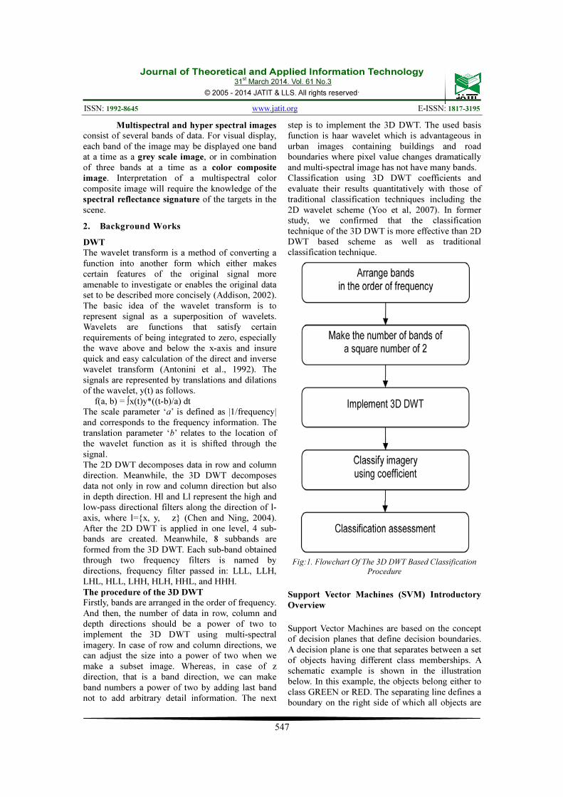
DWT The wavelet transform is a method of converting a function into another form which either makes certain features of the original signal more amenable to investigate or enables the original data set to be described more concisely (Addison, 2002). The basic idea of the wavelet transform is to represent signal as a superposition of wavelets. Wavelets are functions that satisfy certain requirements of being integrated to zero, especially the wave above and below the x-axis and insure quick and easy calculation of the direct and inverse wavelet transform (Antonini et al., 1992). The signals are represented by translations and dilations of the wavelet, y(t) as follows. f(a, b) = ∫x(t)y*((t-b)/a) dt The scale parameter ‘a’ is defined as |1/frequency| and corresponds to the frequency information. The translation parameter ‘b’ relates to the location of the wavelet function as it is shifted through the signal. The 2D DWT decomposes data in row and column direction. Meanwhile, the 3D DWT decomposes data not only in row and column direction but also in depth direction. Hl and Ll represent the high and low-pass directional filters along the direction of l-axis, where l={x, y, z} (Chen and Ning, 2004). After the 2D DWT is applied in one level, 4 sub-bands are created. Meanwhile, 8 subbands are formed from the 3D DWT. Each sub-band obtained through two frequency filters is named by directions, frequency filter passed in: LLL, LLH, LHL, HLL, LHH, HLH, HHL, and HHH. The procedure of the 3D DWT

Firstly, bands are arranged in the order of frequency. And then, the number of data in row, column and depth directions should be a power of two to implement the 3D DWT using multi-spectral imagery. In case of row and column directions, we can adjust the size into a power of two when we make a subset image. Whereas, in case of z direction, that is a band direction, we can make band numbers a power of two by adding last band not to add arbitrary detail information. The next

step is to implement the 3D DWT. The used basis function is haar wavelet which is advantageous in urban images containing buildings and road boundaries where pixel value changes dramatically and multi-spectral image has not have many bands. Classification using 3D DWT coefficients and evaluate their results quantitatively with those of traditional classification techniques including the 2D wavelet scheme (Yoo et al, 2007). In former study, we confirmed that the classification technique of the 3D DWT is more effective than 2D DWT based scheme as well as traditional classification technique.

Fig:1. Flowchart Of The 3D DWT Based Classification

Procedure

Support Vector Machines (SVM) Introductory

Overview

Support Vector Machines are based on the concept of decision planes that define decision boundaries. A decision plane is one that separates between a set of objects having different class memberships. A schematic example is shown in the illustration below. In this example, the objects belong either to class GREEN or RED. The separating line defines a boundary on the right side of which all objects are





548

GREEN and to the left of which all objects are RED. Any new object (white circle) falling to the right is labeled, i.e., classified, as GREEN (or classified as RED should it fall to the left of the separating line).

3. METHODS

3.1. Discrete Wavelet Transform

In numerical analysis and functional analysis, a discrete wavelet transform (DWT) is any wavelet transform for which the wavelets are discretely sampled. As with other wavelet transforms, a key advantage it has over Fourier transforms is temporal resolution: it captures both frequency and location information. The wavelet transform method can be categorized as the discrete wavelet transform (DWT) or the continuous wavelet transform (CWT). Mathematically, the wavelet transform can be represented as

( ) ( ) ( ) ( ) *

,

1, , ,f ab

t bWT ab f t t f t dt

aaψ ψ

+∞

−∞

− = =

∫ ( 1

)

where ( )tf is the signal, a is the scale

parameter, b is the shift parameter, ( )tψ is the mother wavelet.

The CWT allows wavelet transform taking the scale parameter a and shit parameter b to be any real numbers and the DWT only perform wavelet transform with integer shifts b and scales a being the power of two. It is non-redundant, more efficient and is sufficient for exact reconstruction. As a result, the DWT is widely used in data compression and feature

extraction. When we set 1,200== ba , then

( )tψ is changed

( ) ( )kttj

j

kj −=−

−

22 2, ψψ （2）

So, the DWT coefficients can be represented as

() () kjkjkj fdtttfC,,

*

,,ψψ == ∫

+∞

∞−

（3）

A multi-resolution analysis consists of a

sequence of successive approximation spacesj

V .

More precisely, the closed subspacesj

V satisfy

LLL , , , , ,11221110 ++

⊕=⊕=⊕=jjj

WVVWVVWVV

The number j is an integer. The spaces get

bigger when j becomes smaller. When 4=j , we can gain the chart of spaces

From ( )j

Zj

VRL∈

= U2 and

jjjWVV ⊕=

−1 ，we

obtain

( )j

jWRL

∞

−∞=

⊕=2 （4）

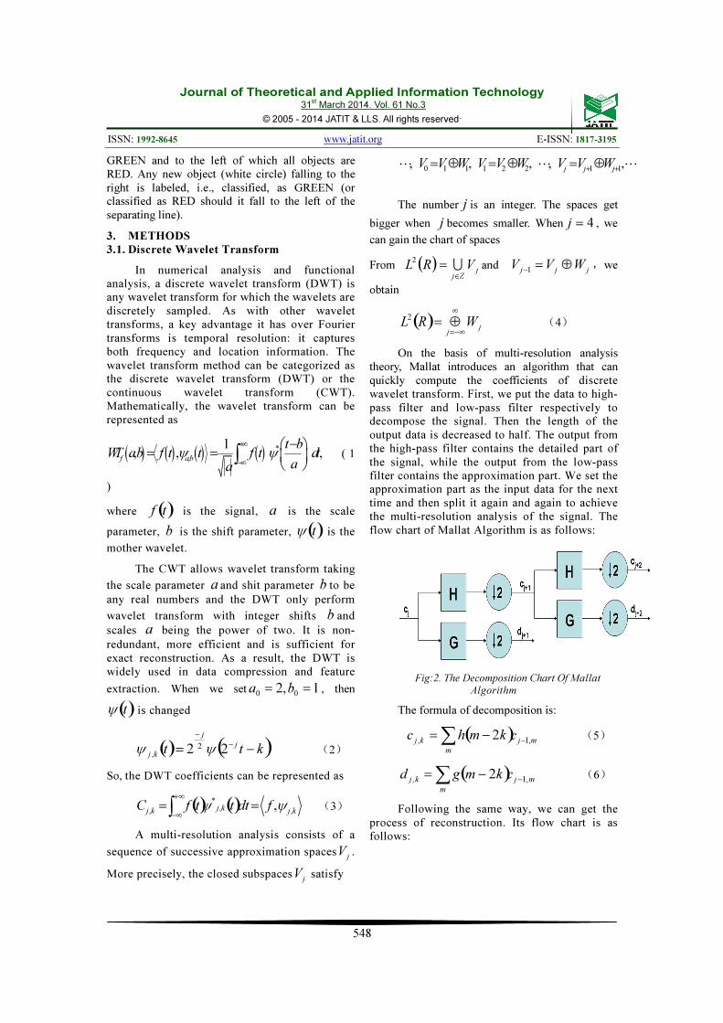
On the basis of multi-resolution analysis theory, Mallat introduces an algorithm that can quickly compute the coefficients of discrete wavelet transform. First, we put the data to high-pass filter and low-pass filter respectively to decompose the signal. Then the length of the output data is decreased to half. The output from the high-pass filter contains the detailed part of the signal, while the output from the low-pass filter contains the approximation part. We set the approximation part as the input data for the next time and then split it again and again to achieve the multi-resolution analysis of the signal. The flow chart of Mallat Algorithm is as follows:

Fig:2. The Decomposition Chart Of Mallat

Algorithm

The formula of decomposition is:

( ) mj

m

kj ckmhc,1,

2−∑ −= （5）

( ) mj

m

kj ckmgd ,1, 2−∑ −= （6）

Following the same way, we can get the process of reconstruction. Its flow chart is as follows:





549

Fig:3. The Reconstruction Chart Of Svm Algorithm

The formula of reconstruction is:

( ) ( ) kj

k

kj

k

mj dkmgckmhc ,,,1 22 ∑∑ −+−=−

（7）

3.2. Spatial Adaptive Algorithm

Assume the largest scale of decomposition is

J . ( )njWf , denotes DWT of signal f at

position n in scale j . Denote the correlation of bordered scale as follows

( ) ( )nijWfnjCorrl

il

,,

1

0

+Π=

−

=

（8）

Where l represents the scale. 1+−< lJj . As the singular of signal increases along with the increase of the scale, bordered points affect each other in the detail scale. We choose 2=l to compute the correlation

( ) ( ) ( )njWfnjWfnjCorr ,1,,2

+⋅= （9）

( )njCorr ,

2 is noted as correlation coefficient of

the position n in scale j .

Although wavelet coefficients are masked up by noise, their correlation coefficients strengthen magnitude along with the increasing scales, so it is easy to distinguish real signal.

To make correlation coefficient and wavelet coefficient more comparable, we define the correlation coefficient uniformly

Discrete wavelet transform based technique is most widely used technique for performing image interpolation. Here DWT is used to decompose a low resolution image into 4 sub band images LL, LH, HL and HH. All the obtained low and high-frequency components of image are then interpolated. A difference image

is obtained by subtracting the interpolated LL image from the original LR image. This difference image is then added to the interpolated high frequency components to obtain estimated form of HF sub band images. Finally IDWT is used to combine these estimated images along with the input image to obtain high resolution images.

In the below figure shows the process transforms the data in the x-direction. Next, the low and high pass outputs both feed to other filter pairs, which transform the data in the y direction. These four output streams go to four more filter pairs, performing the final transform in the z-direction. The process results in 8 data streams. The approximate signal, resulting from scaling operations only, goes to the next octave of the 3-D transform.

3.3. DWT-Based Resolution Enhancement

As it was mentioned before, resolution is an important feature in satellite imaging, which makes the resolution enhancement of such images to be of vital importance as increasing the resolution of these images will directly affect the performance of the system using these images as input. The main loss of an image after being resolution enhanced by applying interpolation is on its high-frequency components, which is due to the smoothing caused by interpolation. Hence, in order to increase the quality of the enhanced image, preserving the edges is essential. In this paper, DWT has been employed in order to preserve the high-frequency components of the image. DWT separates the image into different sub band images, namely, LL, LH, HL, and HH. High-frequency sub bands contain the high-frequency component of the image. The interpolation can be applied to these four sub band images. In the wavelet domain, the low-resolution image is obtained by low-pass filtering of the high-resolution image. The low-resolution image (LL sub band), without quantization (i.e., with double precision pixel values) is used as the input for the proposed resolution enhancement process. In other words, low-frequency sub band images are the low resolution of the original image. Therefore, instead of using low-frequency sub band images, which contains less information than the original input image, we are using this input image through the interpolation process. Hence, the input low-resolution image is interpolated with the half of the interpolation factor, α/2, used to interpolate the high frequency sub bands. In order to preserve more edge information





550

i.e., obtaining a sharper enhanced image, we have proposed an intermediate stage in high-frequency sub band interpolation process. The low-resolution input satellite image and the interpolated LL image with factor 2 are highly correlated. The difference between the LL sub band image and the low-resolution input image are in their high-frequency components. Hence, this difference image can be use in the intermediate process to correct the estimated high-frequency components. This estimation is performed by interpolating the high-frequency sub bands by factor 2 and then including the difference image (which is high-frequency components on low resolution input image) into the estimated high-frequency images, followed by another interpolation with factor α/2 in order to reach the required size for IDWT process. The intermediate process of adding the difference image, containing high-frequency components, generates significantly sharper and clearer final image. This sharpness is boosted by the fact that, the interpolation of isolated high-frequency components in HH, HL, and LH will preserve more high-frequency components than interpolating the low-resolution image directly.

We begin by defining the wavelet series

expansion of function ( )2( )f x L∈ R relative to

wavelet ( )xψ and scaling function ( )xφ . We can write

0 0

0

, ,

( ) ( ) ( ) ( ) ( )j j k j j k

k j j k

f x c k x d k xφ ψ∞

=

= +∑ ∑∑ (

10 )

where 0j is an arbitrary starting scale and the

0

( )j

c k ’s are normally called the approximation or

scaling coefficients, the ( )j

d k ’s are called the

detail or wavelet coefficients. The expansion coefficients are calculated as

0 0 0, ,

( ) ( ), ( ) ( ) ( )j j k j kc k f x x f x x dxφ φ= = ∫% % (

11)

, ,

( ) ( ), ( ) ( ) ( )j j k j kd k f x x f x x dxψ ψ= = ∫% % (

12 ) If the function being expanded is a sequence of numbers, like samples of a continuous function ( )f x . The resulting coefficients are called the discrete wavelet transform (DWT) of ( )f x . Then the series expansion defined in Eqs.

(13) and (14) becomes the DWT transform pair

0

1

0 ,

0

1( , ) ( ) ( )

M

j k

x

W j k f x xM

φ φ−

=

= ∑ % ( 13 )

1

,

0

1( , ) ( ) ( )

M

j k

x

W j k f x xM

ψψ

−

=

= ∑ % ( 14 )

for 0

j j≥ and

0

0

0 , ,

1 1( ) ( , ) ( ) ( , ) ( )j k j k

k j j k

f x W j k x W j k xM M

φ ψφ ψ∞

=

= +∑ ∑∑

( 175)

where ( )f x , 0,

( )j k xφ , and ,

( )j k xψ are

functions of discrete variable x = 0, 1, 2, ... , M − 1.

4. Result Analysis

In this paper, Support Vector Machine (SVM) is a classier method that performs classification tasks by constructing hyper planes in a multidimensional space that separates cases of different class labels. SVM supports both regression and classification tasks and can handle multiple continuous and categorical variables. SVM is better compare with DWT and HW. The DWT performance between 2D and 3D is shown in table 1.

Forest

water

Grass

R or C

Bare soil

Field

original

79.64

75.61

26.74

78.72

19.14

24.61

2D DWT

81.47

82.23

27.22

80.78

19.01

27.67

3D DWT

82.11

83.53

25.95

81.69

18.91

27.82

Table 1: Svm Analysis Method

Fig:4. This Image Graph Shows The Contrast

Between Dwt And He. In Dwt The Processed

Image Looks Like A Natural One But In He It’s A





551

Unnatural Image. And Also He Does Not Support

The Digital Images, But In Dwt Support Digital

Images.

Fig:5. This Image Graph Shows The

Brightness Between DWT And SVD, The

Brightness Of A SVD Is High Compare To

DWT But It Does Not Provide The Clear

View Of The Optimized Location. So The

Processed Image Looks Blurred One.

Fig:6. This Image Graph Deals With Both The

Brightness And Contrast Of A Satellite Image

Because The DWT Support A Contrast And SVM

Support A Brightness As Well As A Clear View

Of A Particular Optimized Location Of A Sensed

Image. SVM Is Better Compare To HE And SVD.

Fig:7. This Image Graph Compare The

Performance Between SVM, DWT And HE,

DWT. At The Result SVM DWT Produce A Good

Performance Behalf Of HE DWT. The SVM

Overcome A Unnatural Looks Of A Processed

Image.

5. CONCLUSION

In this paper, the problem of noise removal, contrast and brightness is handled successfully with the help of these techniques DWT with 3D and SVM. The DWT with 3D increase the contrast compare with 1D and 2D. The proposed technique SVM demonstrates that both regression and classification tasks and can handle multiple continuous and categorical variables. In this SVM classification tasks is handled by a methods called boundary value selection and interior point. In boundary value selection is used to separate items which are having same color. With the above techniques IDWT has been implemented to increase the sharpness and resolution of the satellite image.

REFERENCES

[1]. The University of Southwestern Louisiana ‘Architectures for the 3-d discrete wavelet transform’ Michael Clark Weeks Spring 1998.

[2]. O.Harikrishna, A.Maheshwari ,‘Satellite Image Resolution Enhancement using DWT Technique’, November 2012.

[3]. K. Narasimhan, V. Elamaran, Saurav Kumar, Kundan Sharma and Pogaku Raghavendra Abhishek ,‘Comparison of Satellite Image Enhancement Techniques in Wavelet Domain’April 2012.

[5]. Hee-Young Yoo, Kiwon Lee, and Byung-Doo Kwon ‘Application of the 3D Discrete Wavelet Transformation Scheme to Remotely Sensed Image Classification’ jan 2007.





552

[6]. D. Napoleon, S.Sathya and M.Siva Subramanian ‘Remote sensing image Compression using 3d-spiht Algorithm and 3d-owt’,may 2012.

[7]. Carlos A. Torres ,’Mineral Exploration Using GIS and Processed Aster Images’, Advance GIS EES 6513 (Spring 2007) University of Texas at San Antonio.

[8]. Dr robert sanderson ,’Introduction to remote sensing’New mexico state university. Introduction to Remote Sensing and Image Processing.

[9]. C. Ünsalan, K.L. Boyer, ‘Remote Sensing Satellites and Airborne Sensors’, 2011.

11 20968 kathirvel r 3d based remote sensing image ... · the ground surface area that forms one...

Documents