10/11/2017 - uw - laramie, wyoming | university of wyoming · · 2017-10-1210/11/2017 1 chapter 6...

10/11/2017

1

Chapter 6

1. Discuss three US labor market trends since 19602. Use supply and demand to explain the labor market3. Use supply and demand to explain employment and

real wage trends since 19604. Define and calculate the unemployment rate and the

labor force participation rate5. Define and discuss three types of unemployment and

their costs to individuals and society.

6-2

• Industrialized countries have enjoyed real earnings growth in the 20th century

6-3

• U.S. real earnings are about twice real earnings in 1960

2010

• U.S. real earnings are nearly five times real earnings in 1929

2010

©McGraw-Hill Education. All rights reserved.

17-4

• The graph shows that average hourly earnings for employees (and self-employed people) doubled since 1960


17-5

• However, the growth in real wages for over half of American workers slowed since 1970

• while the total number or workers and the percent of the population that works increased

• Data on real wage growth:– 1960 – 1973 2.5% per year– 1973 – 1995 -.75% per year– 1996 – 2010 1% per year– 1970 – 2012 0% per year

6-6

10/11/2017

2


17-7

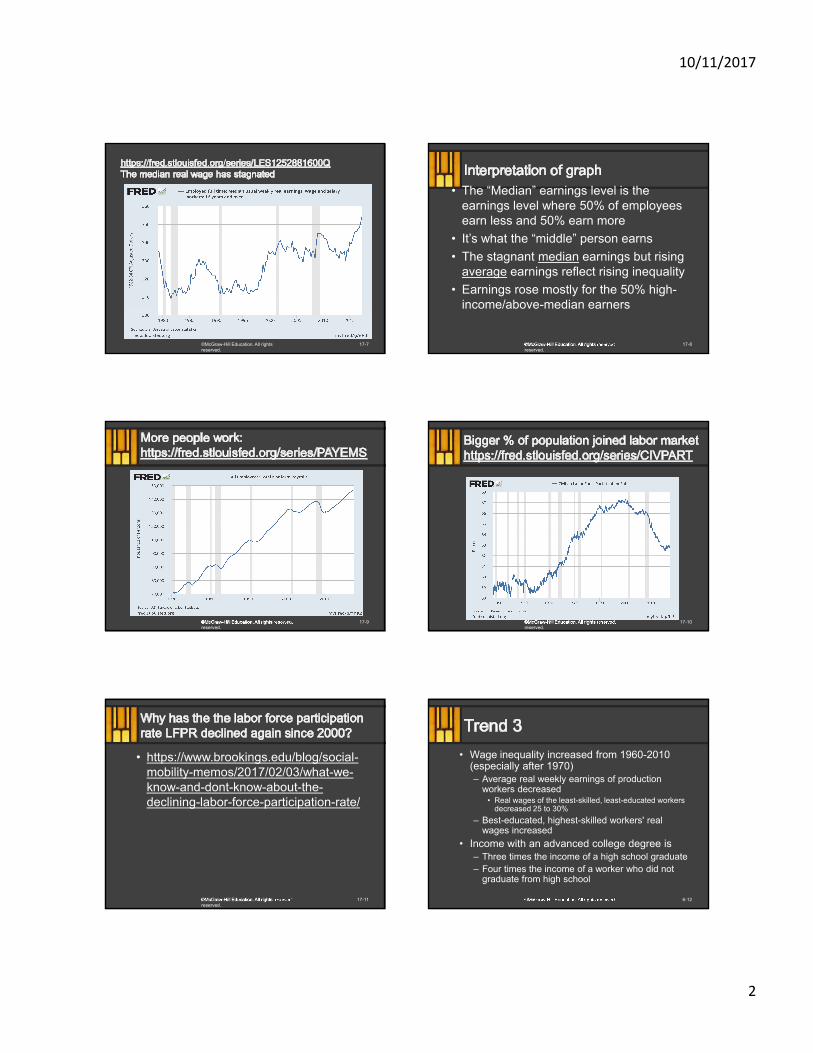
• The “Median” earnings level is the earnings level where 50% of employees earn less and 50% earn more

• It’s what the “middle” person earns• The stagnant median earnings but rising

average earnings reflect rising inequality• Earnings rose mostly for the 50% high-

income/above-median earners


17-8


17-9 ©McGraw-Hill Education. All rights reserved.

17-10

• https://www.brookings.edu/blog/social-mobility-memos/2017/02/03/what-we-know-and-dont-know-about-the-declining-labor-force-participation-rate/


17-11

• Wage inequality increased from 1960-2010 (especially after 1970)– Average real weekly earnings of production

workers decreased• Real wages of the least-skilled, least-educated workers

decreased 25 to 30%– Best-educated, highest-skilled workers' real

wages increased• Income with an advanced college degree is

– Three times the income of a high school graduate– Four times the income of a worker who did not

graduate from high school

6-12

10/11/2017

3



17-14

• http://www.epi.org/publication/charting-wage-stagnation/


17-15

• Supply and demand analysis can be used to find the price of labor (the real wage) and the quantity supplied (the employment level)

• The labor market is an input market where firms demand (or buy) labor to produce goods and services; and individuals supply (or sell) labor to earn income

6-16

• The demand for labor depends upon– The productivity of workers– The price of the workers’ outputWhen workers produce more or the output sells for higher prices, labor demand rises.

6-17

• We normally assume diminishing returns to labor

• Diminishing returns means that, holding equipment and other inputs constant, each additional worker adds less to production than the previous worker

• The Value of the Marginal Product (VMP) is the extra revenue an added worker generates


17-18

10/11/2017

4

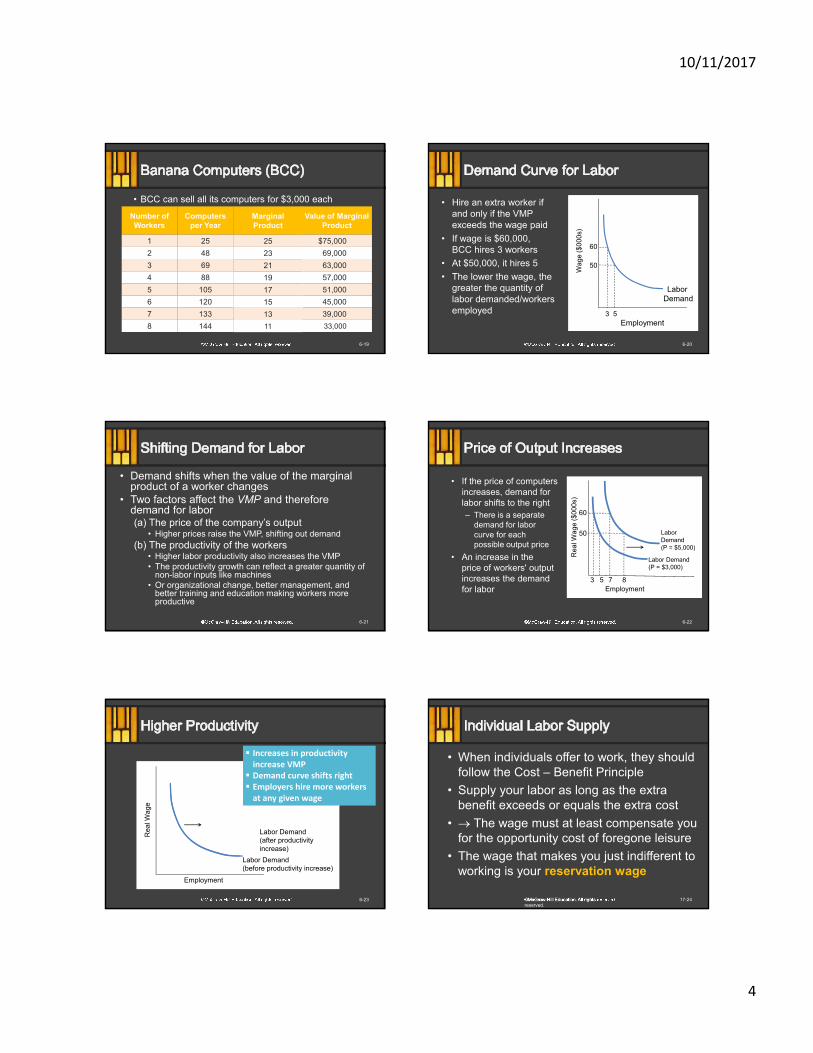
Number of Workers

Computers per Year

1 252 483 694 885 1056 1207 1338 144

6-19

Value of Marginal Product

$75,00069,00063,00057,00051,00045,00039,00033,000

Marginal Product

2523211917151311

• BCC can sell all its computers for $3,000 each • Hire an extra worker if and only if the VMP exceeds the wage paid

• If wage is $60,000, BCC hires 3 workers

• At $50,000, it hires 5• The lower the wage, the

greater the quantity of labor demanded/workers employed

6-20

Employment

Wag

e ($

000s

)

Labor Demand

3

60

50

5

• Demand shifts when the value of the marginal product of a worker changes

• Two factors affect the VMP and therefore demand for labor(a) The price of the company’s output

• Higher prices raise the VMP, shifting out demand(b) The productivity of the workers

• Higher labor productivity also increases the VMP• The productivity growth can reflect a greater quantity of

non-labor inputs like machines• Or organizational change, better management, and

better training and education making workers more productive

6-21

• If the price of computers increases, demand for labor shifts to the right– There is a separate

demand for labor curve for each possible output price

• An increase in the price of workers' outputincreases the demand for labor

6-22

Employment

Rea

l Wag

e ($

000s

)

Labor Demand(P = $3,000)

60

3

50

5 7 8

Labor Demand(P = $5,000)

6-23

Increases in productivity increase VMP Demand curve shifts right Employers hire more workers

at any given wage

Employment

Rea

l Wag

e

Labor Demand(before productivity increase)

Labor Demand(after productivityincrease)

• When individuals offer to work, they should follow the Cost – Benefit Principle

• Supply your labor as long as the extra benefit exceeds or equals the extra cost

• The wage must at least compensate you for the opportunity cost of foregone leisure

• The wage that makes you just indifferent to working is your reservation wage


17-24

10/11/2017

5

• If working conditions are unpleasant or dangerous, a premium for that would be included in the wage

6-25 6-26

Employment

Rea

l Wag

e

Labor Supply

The labor supply curve slopes up because at a higher real wage, (a) more people are willing to work(b) existing workers are willing to work longer hours

• What determines the economy-wide or macroeconomic labor supply?

1. The size of the working age population(#non-institutionalized 16+ aged individuals)2. The share of the working-age population that is willing to work

6-27

• The US has ~225 million people aged 16+ and 150 million willing to work

• The labor force participation rate LFPR is about 2/3

• The size of the labor force responds to population growth (natural + net immigration) and the ages where people start working and retiring


17-28

• A shift in labor supply is caused by any change in the number of workers willing to work at each wage– Increase in the working-age population

• A Baby Boom (like after WW 2, lots of babies born)• Higher net immigration• Increasing age at retirement

– Increase in the share of working-age population willing to work

• Women's participation in the labor force has increased in the last 50 years

6-29

• Industrialized countries have had sustained growth in productivity in the 20th

centuryThis increased demand for labor and explains why real wages and employment increased since 1960

• Productivity increases were due to– Technological progress– Increases in capital

equipment

6-30

Employment

Rea

l Wag

e

S

D

W

N

W'

N'

D'

10/11/2017

6


17-31

Average Growth Rate (%)Productivity Real Earnings

1970 – 1979 1.92% 0.00% 1980 – 1989 1.47 -0.811990 – 1999 2.03 0.342000 – 2009 2.57 0.72

• Stagnant growth in real wages for most US workers since 1970 could be due to – Slower growth in demand for labor – Faster growth in the supply of labor

6-32

• Slower demand growth for labor should lead to limited job creation

• Yet, total employment grew rapidly • The supply of labor increased as well.

– Increased participation by women– Baby Boomers (born after WW2) entered

labor force around 1970.– High immigration since 1970

6-33

• Exercise: show that limited growth in labor demand (outward demand shifts) coupled with increased labor supply (outward supply shifts) can explain both:

• (a) stagnant real wages • (b) employment growth


17-34

• The large baby-boomer generation (born ca. 1945-50) is now retiring

• The growth in labor supply as women joined the labor force is leveling off as large % has joined

• The labor force participation rate (% of people aged 16+ working or looking for work) has declined since 2000


17-35

• If the growth in labor supply slows down and labor demand grows stably/picks up because of technology and education making the workers more productive, we should expect faster real-wage growth – but it’s hard to predict


17-36

10/11/2017

7

• Globalization = stronger connection and integration with other countries, in terms of trade, investment, culture etc.

• It allows countries to specialize and exploit Comparative Advantage (Chapter 2)

• But ex. production of low-skilled, labor-intensive goods has moved abroad

• This decreased demand for unskilled US workers and their wages

6-37 6-38

Employment

Rea

l Wag

e

Employment

ST

DT

W

NT

SS

DS

NS

D'T

W’T

N'T

D'S

W'S

N'S

SoftwareTextiles

• One source of rising inequality can be globalization as skilled wages rise (ex. for the software sector) and unskilled wages (ex. for the textile sector) fall

• Economists do not recommend shutting off to trade b/c the US as a whole benefits from specializing in its comparative advantage industries (Chapter 2)

6-39

• The best policy is to let the workers who lose their jobs move to the comparative advantage industries (from textiles to software) or new geographical regions where jobs are found

• Transition aid by government can assist workers to make the change, retrain and reeducate


17-40

• Another cause of increasing wage inequality is technological change

• Because technology may be “skill-biased” and favor the higher-skilled or better-educated

• Automatic check-out at supermarket or robots can lower demand for unskilled workers

6-41

• Computer and management innovations (like new accounting techniques or better access to economic data) can favor college-educated people who can better use it

• Demand for “skilled” labor goes up, demand for “unskilled” labor decreases


17-42

10/11/2017

8

6-43

Employment

Rea

l Wag

e

Unskilled Workers

W'S

N'U

SU

DU

NU

WS

Employment

Skilled Workers

D'S

SS

NS

WS

DSD'U

N'S

W'S

Une

mpl

oyed

• Bureau of Labor Statistics (BLS) estimates employment and unemployment monthly

• Labor force = employed + unemployed• Unemployment rate = unemployed / labor force• Participation rate = labor force / population 16+

Out of the

Labor Force

6-44

Population Age 16+

Employed

U.S. Employment Data, August 2014 (in millions)Employed 146.37 millionUnemployed 9.59 millionLabor Force 155.96 millionNot in the Labor Force 92.27 millionWorking-Age Population 248.23 millionUnemployment Rate 6.1%Participation rate 62.8%


17-46

6-47

• Economic costs: Lost production(the GDP loss equals the wage loss plus the profit loss)

• Psychological costs– Individual self-esteem– Family stress and increased uncertainty

• Additional social costs (other cost to society)– Potential increases in crimes and social problems– Use scarce public resources to address these

problems and assist the unemployed

6-48

10/11/2017

9

• Costs of unemployment are directly related to the length of time a person has been unemployed– Unemployment spell is the period during which

an individual is continuously unemployed– Duration of unemployment is the length of the

unemployment spell• The unemployed population in April 2011:

6-49

Duration (weeks) 5 or less 5 – 14 More than 14% of unemployed 20% 22% 58%

• People who have been out of work for 6+ months are long-term unemployed

• People that continuously mix short-term or temporary jobs with unemployment are chronically unemployed

• People who want to work but gave up looking are discouraged workers

6-50

• Involuntary part-time workers are people who like to work full-time but cannot find full-time jobs

• The August 2014 unemployment rate was 6.1%• But if we add the discouraged workers and

involuntary part-time workers, it would be 12%

6-51

• Frictional unemployment occurs when workers are between jobs– Short duration, low economic cost– May increase economic efficiency b/c you

move to a better match• Cyclical unemployment is the

increase in unemployment during economic slow-downs (recessions)– Usually short duration also

6-52

• Structural unemployment is long-term, chronic unemployment in a well-functioning economy– Lack of skills, language barriers, or discrimination– Structural shifts in production create a long-term

mismatch between workers and market needs– Regulations and other employment barriers:

• Minimum wages ■ Unions ■ Unemployment Insurance

– High economic, psychological, and social costs– Example: U.S. steel and manufacturing sectors

due to loss of international comparative advantage

6-53 6-54

Employment

Rea

l Wag

e

D

S

N

W

AWmin

NA

B

NB

Minimum Wage Laws

• Setting a minimum wage (Wmin) above equilibrium (W) creates (NB – NA) unemployment

• Workers who find a minimum-wage job get a higher wage

• Others are unemployed

10/11/2017

10

• Labor union benefits– Improve wages and

working conditions– Promote democracy

and dialogue in the workplace as employers and unions make joint decisions

6-55

• Labor union costs– The high wages

discourage hiring and create unemployment

– Decrease companies’ international competitiveness, raise consumer prices

– Strikes and production disruptions

• Unemployment insurance is a government transfer to unemployed workers– Helps to reduce the costs of unemployment– May give the unemployed an incentive to

search longer and less intensely• To work efficiently, unemployment benefits

should be– For a limited time– Less than the income received when working

6-56

• Health and safety regulations can reduce the demand for labor by– Increasing employer costs– Reducing productivity

• The reduction in demand will increase unemployment and lower wages

• It’s a trade-off between the benefits and costs to society

6-57 6-58

Three Trends

Labor Market

Demand for Labor

Supply of Labor

Unemployment

Costs

Types

10/11/2017 - uw - laramie, wyoming | university of wyoming · · 2017-10-1210/11/2017 1 chapter 6...

Documents