10 Digital Audio Compression

The compression of digital audio data is an important topic these days. Compressing (reducing) thedata storage requirements of digital audio allows us to fit more songs into our iPods and downloadthem faster. We will apply ideas from interpolation, least squares and other topics to reduce thestorage requirements of digital audio files. All of our approaches will replace the original audio signalwith approximations that are made from a linear combination of cosine functions.

You will learn the basic ideas behind data compression methods used in mp3 and other algo-rithms. You’ll also encounter several interesting MATLAB/Octave commands in the course of thisproject, including commands for manipulating sound.

Computers and sound

Sound is a complicated phenomenon. It’s normally caused by a moving object in air (or othermedium), for example a loudspeaker cone moving back and forth. The motion in turn causes airpressure variations that travel through the air like waves in a pond. Our eardrums convert thepressure variations into the phenomenon that our brain processes as hearing.

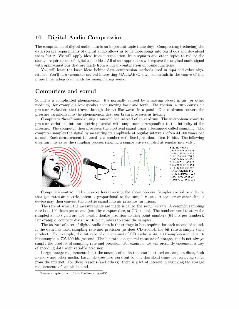
Computers “hear” sounds using a microphone instead of an eardrum. The microphone convertspressure variations into an electric potential with amplitude corresponding to the intensity of thepressure. The computer then processes the electrical signal using a technique called sampling. Thecomputer samples the signal by measuring its amplitude at regular intervals, often 44,100 times persecond. Each measurement is stored as a number with fixed precision, often 16 bits. The followingdiagram illustrates the sampling process showing a simple wave sampled at regular intervals1:

Computers emit sound by more or less reversing the above process. Samples are fed to a devicethat generates an electric potential proportional to the sample values. A speaker or other similardevice may then convert the electric signal into air pressure variations.

The rate at which the measurements are made is called the sampling rate. A common samplingrate is 44,100 times per second (used by compact disc, or CD, audio). The numbers used to store thesampled audio signal are not usually double-precision floating-point numbers (64 bits per number).For example, compact discs use 16 bit numbers to store the samples.

The bit rate of a set of digital audio data is the storage in bits required for each second of sound.If the data has fixed sampling rate and precision (as does CD audio), the bit rate is simply theirproduct. For example, the bit rate of one channel of CD audio is 44, 100 samples/second × 16bits/sample = 705,600 bits/second. The bit rate is a general measure of storage, and is not alwayssimply the product of sampling rate and precision. For example, we will presently encounter a wayof encoding data with variable precision.

Large storage requirements limit the amount of audio that can be stored on compact discs, flashmemory and other media. Large file sizes also work out to long download times for retrieving songsfrom the internet. For these reasons (and others), there is a lot of interest in shrinking the storagerequirements of sampled sound.

1Image adapted from Franz Ferdinand, c©2005

Least-squares data compression

Least-squares data fitting can be thought of as a method for replacing a (large) set of data with amodel and a (smaller) set of model coeffcients that approximate the data in anoptimal way–namely, by minimizing the Euclideannorm of the residual difference between the data andthe model.

Consider the following simple example. Let thefunction f(t) = cos(t)+5 cos(2t)+cos(3t)+2 cos(4t).A plot of f(t) for 0 ≤ t ≤ 2π appears as the bluecurve in the figure. Let’s say we are given a dataset of 1000 discrete function values of f(t) regularlyspaced over the interval 0 ≤ t ≤ 2π. We can fullyinterpolate the data by setting up the model matrixA (using MATLAB/Octave notation):

t = linspace (0,2*pi,1000)’;b = cos(t) + 5*cos(2*t) + cos(3*t) + 2*cos(4*t);A = [ones(size(t)), cos(t), cos(2*t), cos(3*t), cos(4*t)];

and then solving the linear system Ax = b with the command x=A\b. Try it! Note that the solutionvector components match the function coefficients.

Some of the coefficients are not as large as others in this simple example. We can approximatethe function f with a least-squares approximation that omits parts of the model corresponding tosmaller coefficients. For example, set up the least-squares model

A = [cos(2*t), cos(4*t)];

and solve the corresponding least-squares system x=A\b. This model uses only two coefficients todescribe the data set of 1000 data points. The resulting fit is reasonable, and is displayed by the redcurve in the figure. The plot was made with the command plot (t,b,’-b’,t,A*x,’-r’).

The cosine function oscillates with a regular frequency. The multiples of t in the above examplecorrespond to different frequencies (the larger the multiple of t is, the higher the frequency ofoscillation). The least-squares fit computed the best approximation to the data using only twofrequencies.

Exercise

Experiment with different least-squares models for the above example by omittingdifferent frequencies. Plot your experiments and briefly describe the results.

Manipulating sound in MATLAB and Octave

MATLAB and Octave provide lots of commands that make it relatively easy to read in, manipu-late, and listen to digital audio signals. Accompanying this project, you will find a short sound file:http://www.math.kent.edu/ blewis/numerical computing.1/project5/shostakovich.wav. Thefile is sampled at 22,050 samples per second and 16 bits per sample (exactly 1/2 the bit rate of CDaudio), and is about 40 seconds long. If you don’t care for the tune, you are free to experiment withany audio samples that you wish. In order to experiment with the provided file, you will need todownload it from the above link into your working directory.

The MATLAB/Octave command to load an audio file is:

[b,R] = wavread (’shostakovich.wav’);N = length(b);

The returned vector b contains the sound samples (it’s very long!), R is the sampling rate, and N isthe number of samples. Note that, even though the precision of the data is 16 bits, MATLAB andOctave represent the samples as double-precision internally. You can listen to the sample you justloaded with the command:

sound (b,R);

Some versions of MATLAB and Octave may have slightly different syntax–use the help commandfor more detailed information. The wavread command for Octave is part of the Octave-Forge project.

Sampled audio data is generally much more complicated looking than the simple example in thelast section, confirmed by viewing the data with the command plot(b) (try it!). However, it toocan be interpolated and/or least-squares fit with a cosine model:

y = c0 + c1 cos ω1t + c2 cos ω2t + · · ·+ cn−1ωn−1t,

for some positive integer n− 1 and frequencies ωj . A famous and important result from informationtheory called the Shannon-Nyquist theorem requires that the highest frequency in our model, ωn−1,be less than half the sampling rate. That is, our cosine model assumes that the audio data is filteredto cut-off all frequencies above half the sampling rate.

The cosine model requires additional technical assumptions on the data. Recall that the cosinefunction is an even function, and the sum of even functions is an even function. Therefore, themodel also assumes that the data is even. The usual approach taken to satisfy this requirement ofthe model is to simply assume that the data is extended outside of the interval of interest to makeit even.

The above-mentioned conditions (cut-off frequency, extension beyond the interval boundaries)are in general important to consider, but we won’t get in to the details in this project. Instead, wefocus on the basic ideas behind compression methods like mp3.

Computing the model interpolation coefficients with the DCT

Let the vector b contain one second of sampled audio, and assume that the sampling rate is Nsamples per second (b is of length N). It’s tempting to proceed just as in the simple example aboveby setting up an interpolation model

t = linspace (0,2*pi,N)’;A = [ones(size(t)), cos(t), cos(2*t), cos(3*t), ..., cos((N/2-1)*t)];x = A\b;

Aside from a few technical details, this method could be used to interpolate an audio signal. However,consider the size of the quantities involved. At the CD-quality sampling rate, N = 44100, and thematrix A is gigantic (44100× 22050)! This problem is unreasonably large.

Fortunately, there exists a remarkable algorithm called the Fast Discrete Cosine Transform (DCT)that can compute the solution with extreme efficiency. The DCT is a variation on the famous fastFourier transform (FFT) that we will study in greater depth next semester. The DCT producesscaled versions of the model coefficients for us with the command:

c = dct(b);

The returned coefficient vector c is of the same length as b.To investigate the plausibility of the DCT, we can try it out on our simple example:

% Simple example revisitedt = linspace (0,2*pi,1000)’;b = cos(t) + 5*cos(2*t) + cos(3*t) + 2*cos(4*t);x = dct(b);N = length(b);w = sqrt(2/N);f = linspace(0, N/2, N)’;plot (f(1:8),w*x(1:8),’x’);

The variable w is a scaling factor produced by the DCT algorithm and the vector f is the frequencyscale for the model coefficients computed by the DCT and stored in x. The frequency range from0 to N/2 − 1 corresponds to half the sampling rate (assumed here to be N). We can think of thedct(b) command as essentially computing A\b for the full interpolation model using the frequenciesin the vector f . Your plot should show that we closely compute the model coefficients (i.e., a valueof 1 at frequency 1, 5 at frequency 2, etc.)

We can reconstruct the original signal from the model coefficients with the command:

y = idct(x); % The reconstructed data is in y.plot (t, b, ’-r’, t, y,’-b’);

The plots should overlay each other. The idct command is the inverse of the dct command. We canthink of idct(x) as computing the product Ax for an appropriate model matrix A and coefficientvector x.

Digital filtering

The DCT algorithm can be used to not only interpolate data, but to compute a least-squares fit tothe data by omitting frequencies. The process of computing a least-squares fit to digitized signals byomitting frequencies is called digital filtering. Digital filtering can reduce the storage requirementsof digital audio by simply lopping off parts of the data that correspond to specifc frequencies. Ofcourse, cutting out frequencies affects the sound quality of data. However, the human ear is notequally sensitive to all frequencies. In particular, we generally don’t perceive very high and very lowfrequencies nearly as well as mid-range frequencies. In some cases, we can filter out these frequencieswithout significantly affecting quality. An easy way to filter specific frequencies in MATLAB andOctave is to generate a mask. Consider this example:

[b,R] = wavread (’shostakovich.wav’);N = length(b);c = dct(b); % Compute the interpolation model coefficientsw = sqrt(2/N);f = linspace(0,R/2,N)’;plot (f,w*c); % Shows a plot of the frequencies coefficients for the sample% Generate a mask of zeros and ones. m is 0 for every frequency above 3000, 1 otherwise.% This mask will cut-off all frequencies above 3000 cycles/second.m = (f<3000);plot (f,w*m.*c); % Display the filtered frequency coefficients.y = idct(m.*c); % Generate a filtered sound sample data setsound(y,R); % Listen to the result

Exercise

Experiment with several frequency cut-off values in the above example. Listen to yourresults.

Exercise

Exhibit how to construct a single mask that will cut off frequencies below 200 and above5000 cycles/second.

Exercise

How much does the above code reduce the storage requirement of the sample (in bitrate)?

The ideas behind mp3

Digital filtering is an effective technique for compressing audio data in many situations, especiallytelephony. Cutting out entire frequency ranges is rather a brute-force method, however. There aremore effective ways to reduce the storage required of digital audio data, while also maintaining ahigh-quality sound.

One idea is this: rather than cutting out “less-important” frequencies altogether, we could storethe corresponding model coefficients with lower precision–that is, with fewer bits. This techniqueis called quantization. The “less-important” frequencies are determined by the magnitude of theirDCT model coefficients. Coefficients of small magnitude correspond to cosine frequencies that don’tcontribute much to the sound sample. A key idea of methods like the MP3 algorithm is to focus thecompression on parts of the signal that are perceptually not very important.

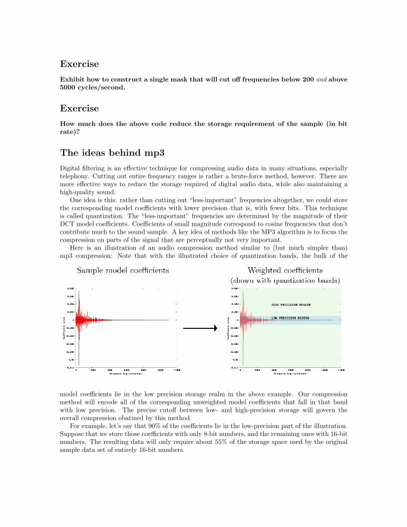
Here is an illustration of an audio compression method similar to (but much simpler than)mp3 compression: Note that with the illustrated choice of quantization bands, the bulk of the

model coefficients lie in the low precision storage realm in the above example. Our compressionmethod will encode all of the corresponding unweighted model coefficients that fall in that bandwith low precision. The precise cutoff between low- and high-precision storage will govern theoverall compression obatined by this method.

For example, let’s say that 90% of the coefficients lie in the low-precision part of the illustration.Suppose that we store those coefficients with only 8-bit numbers, and the remaining ones with 16-bitnumbers. The resulting data will only require about 55% of the storage space used by the originalsample data set of entirely 16-bit numbers.

Exercise

What is the bit rate of the compressed audio sample discussed in the last paragraph,assuming 22,050 samples per second?

We can achieve higher compression by either widening the low-precision region, or by lowering theprecision used to store the coefficients, or both. The algorithm used in mp3 compression uses similartechniques to achieve up to a 10:1 compression of CD audio and still maintain a high perceived qualityof sound.

Quantization in MATLAB and Octave

MATLAB and Octave do not easily represent quantized numbers internally. We can, however,simulate the result of quantization in double-precision with the following function, quantize.m:

function y = quantize (x, bits)

m = max(abs(x));y = x/m;y = floor((2^bits - 1)*y/2);y = 2*y/(2^bits -1);y = m*y;

Exercise

Explain how the quantize.m function works.

MP3-like compression with MATLAB and Octave

The following code example illustrates our discussion of audio data compression with actual audiosamples. You will need the above quantize.m function, as well as the standard perceptual model ofhuman hearing provided in the functions psyweight.m and is0226.m.

% Load an audio sample data set[b,R] = wavread (shostakovich.wav);N = length(b);% Compute the interpolation model coefficientsc = dct(b);w = sqrt(2/N);f = linspace(0,R/2,N)’;% Lets look at the weighted coefficients and pick a cutoff valueplot (f,w*c)% Pick a cutoff value and split the coefficients into low- and high-precision sets:cutoff = 0.00015mask = (abs(w*c)<cutoff);low=mask.*c;high=(1-mask).*c;% This plot nicely illustrates the cutoff region:plot(f,w*high,’-R’,f,w*low,’-b’)% Now pick a precision (in bits) for the low precision data set:lowbits=8% We wont quantize the high-precision set of coefficients (high), only the% low precision part (requires quantize.m):low = quantize(low, lowbits);% Finally, let’s reconstruct our compressed audio sample and listen to it!y=idct(low+high);sound (y,R);

Exercise

Experiment wuth the above code, trying out different cuttoff values and precision values(lowbits). Listen to your results. What is the lowest bit rate that you can find thatstill sounds good to you?