10 comparative risk analysis - who · 10 comparative risk analysis graham mcbride, tom ross and al...

10

Comparative risk analysis

Graham McBride, Tom Ross and Al Dufour

10.1 ESSENTIALS OF RISK ASSESSMENT

Risk assessment is a systematic process to estimate the level of risk related to somespecific action or activity. It is now commonly applied to a wide variety of humanendeavours in which harm to people, the environment or economic interests mightoccur. In the context of public health, the process attempts to quantify thelikelihood and severity of illness to individuals or populations from aspecified hazard.

The primary purpose of risk assessment is to provide support for decisions aboutmanaging risks associated with those specific actions or activities. This is done bysystematically synthesizing information about the factors that contribute to the riskin a coherent framework that enables risk, or relative risk, to be inferred fromknowledge of those risk-contributing factors in specific circumstances.Depending on the needs of the risk manager, the risk assessment may attempt toassess the relative effectiveness of proposed risk mitigations, or to estimate the

© 2012 World Health Organization (WHO). Animal Waste, Water Quality and Human Health. Editedby Al Dufour, Jamie Bartram, Robert Bos and Victor Gannon. ISBN: 9781780401232. Published byIWA Publishing, London, UK.

magnitude of the risk under different circumstances, or the risk to differentpopulations or sub-groups within the population.

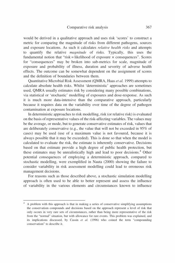
There are many frameworks that describe the interaction between riskassessment1 and risk management, and a third component known as “riskcommunication” which involves understanding the interests, concerns and valuesof “stakeholders”, that is, those affected by the risk, so as to guide and optimizerisk management decisions. One depiction of the interaction among these aspectsof risk analysis is presented in Figure 10.1.

RISK ASSESSMENT

Science-based

RISK COMMUNICATIONInteractive exchange of opinion

and information concerning risk

RISK MANAGEMENT

Policy-based

Figure 10.1 A depiction of the interaction between risk assessors, risk managers and thoseaffected by the risk (‘stakeholders’) within the risk analysis framework developed by the WorldHealth Organization and the Food and Agriculture Organisation of the United Nations. Arrowsindicate lines of communication, while separate circles are intended to depict discrete roles ofthose responsible for risk assessment, those responsible for making decisions about risk, andstakeholders (based on: WHO/FAO 2009).

1 While some organisations consider risk assessment to encompass risk management, riskcommunication and risk analysis, many organisations involved in environmental and public healthrisk assessment consider risk analysis to be the ‘umbrella’ activity that encompasses riskassessment, management and communication. For example, the Society for Risk Analysis (http://www.sra.org) broadly defines risk analysis “…to include risk assessment, risk characterization,risk communication, risk management, and policy relating to risk.” We choose to adopt thisconvention here.

Animal Waste, Water Quality and Human Health362

Risk management involves a balance between the most effective risk mitigationaction, based on cost or technical feasibility, and the interests and values ofstakeholders. Therefore risk managers will also seek information on costs(compared to the benefits) of risk management options. The efficacy of variousapproaches and the factors that affect it may be considered in the riskassessment to support the decisions of risk managers. The combination of riskassessment, risk management and risk communication is, in some frameworks,collectively termed ‘risk analysis’. Microbiological risk assessment frameworksrelevant to waterborne risk are discussed by Haas et al. (1999, Chapter 3);WHO (2003); Gale (2001a&b, 2003), Coffey et al. (2007) and Goss & Richards(2008).

10.1.1 Key elements

The first step in risk assessment usually is the development of a conceptual modelor framework that combines knowledge of risk-affecting factors and how theycould interact to cause harm. In many cases this information can be expressedmathematically as a series of equations that, provided sufficient quantitative dataand knowledge exist, enable quantification of the risk or, at least, the relativerisk. In assessing the public health risk from exposure to microbial pathogens,the “risk assessment” task is often broken down into four discrete components:

• Hazard Identification –which involves describing the hazard (pathogens),presenting the evidence that the hazard causes illness and that it can causeillness from the source of exposure being considered, and the type of illnesscaused.

• Hazard Characterization –which presents information about characteristicsof the organism that affect its ability to cause illness, such as virulencefactors, physiological traits that affect its survival in the environment and,importantly, the severity of disease caused, including consideration ofdifferences in susceptibility of different members of the populationexposed and the probability of illness as a function of the dose ingested.In the context of water and sanitation this corresponds to considerationand characterization of elements of “pathogen virulence” and “hostsusceptibility”. This includes consideration of dose-response relationships,which is sometimes considered as a further discrete component (e.g., Haaset al. 1999).

• Exposure Assessment –which attempts to estimate the exposure of theaffected population(s) to the pathogen under scrutiny. In the context ofpublic health risk from recreational/occupational exposure to water thiscould involve consideration of, for example: sources of contamination,

Comparative risk analysis 363

loads and composition of pathogens in sources of contamination, and factorsthat would increase or decrease the risk of exposure such as inactivation dueto UV irradiation, predation, or human interventions. It should also considerfactors that would alter exposure of different members of the population suchas age (children may swim more often, or ingest more water whenswimming), cultural and gender factors (e.g., women in developing nationsmay be more likely to be exposed due to their domestic responsibilities),type of water exposure (e.g., full immersion through swimming cf.accidental exposure through clothes-washing). In the context of water andsanitation this corresponds to consideration and characterization ofelements of load, transport and exposure (see: Chapters 2–7).

• Risk Characterization – the systematic and scientific process of synthesizingall the relevant knowledge and information to produce estimates of risk, orrelative risk.

10.1.2 Principles of risk assessment

Ideally, the model and the data and knowledge that it is based on will be clearlydocumented, or ‘transparent’. Usually, however, insufficient knowledge and dataare available to enable unambiguous assessment of (comparative) risk, ordecisions based on that risk, and a number of assumptions will need to be madein the development and application of the risk assessment model. Theseassumptions, and their potential consequences for the decisions based on them,should also be clearly articulated.

10.1.3 Pathogen selection

Many zoonotic pathogens have been reported in the literature as the causal agentsof human infections or outbreaks of disease. The majority of these humaninfections were transmitted from animals to humans by food products (O’Brien2005). Several outbreaks have been transmitted by drinking-water and only asmall number have been transmitted by recreational water (Craun 2004).Outbreaks may, however, comprise only a minority of the actual cases suffered:“…probably the vast majority of waterborne disease burden arises outside ofdetected outbreaks” (Bartram 2003). The zoonotic bacterial pathogensmentioned most frequently are E. coli O157, Campylobacter, Salmonella,Leptospira and Listeria. Protozoan pathogens include Cryptosporidium, Giardiaand Toxoplasma (Schlundt et al. 2004, Pell 1996, Rosen 2000, Bicudo & Goyal2003). Although most of the zoonotic pathogens have been associated withsporadic and outbreak patterns of disease, a few have not been associated with


waterborne outbreaks or with faecal contamination of water. The following criteriahave been adopted whereby pathogens from the list above will be selected forinclusion in our risk comparison process.

• The pathogens are known to be carried by animal or bird species;• The pathogens are discharged in the faeces of animals or birds;• The pathogens have been isolated from surface waters;• The pathogens cause disease in humans.

The zoonotic pathogens that meet these criteria are:

E. coli O157 (more generally, EHEC) which are predominantly carried byruminants including beef and dairy cattle and sheep (USEPA 2000a, Caprioliet al. 2005) and, to a lesser extent, monogastric animals (Chapman 2000,Chapman et al. 1997). This organism has been associated with outbreaks ofdisease that are related to recreational water (e.g. Keene et al. 1994) and hasbeen isolated from surface waters. None of the outbreaks have been linkeddirectly to direct contacts with animals. However, some have been associatedwith food and drinking-water.

Campylobacter species are frequently found in surface waters and this organism iscarried by poultry, cattle and sheep (Jones 2001). Campylobacter has frequentlybeen linked to outbreaks transmitted by food and water, but its occurrence ispredominated by sporadic and endemic patterns, rather than outbreaks. InNew Zealand, where campylobacteriosis is a reportable disease, about 300 to400 cases per hundred thousand population have been reported in recent years(Till & McBride 2004, Till et al. 2008).2 In western and northern Europe, inthe late 1990s reported rates per 100,000 varied from ∼20 (The Netherlands)to ∼100 (England Wales) (Kist, 2002). Annual reported incidence in Australiais ∼100/100,000 (NNDSS, 2010) and in Canada seems to be declining but atthe time of writing is ∼30/100,000 (PHAC, 2010). It is important to note thatthe actual incidence of this disease in the USA is estimated to be ∼40 timeshigher than the reported rate (Mead et al., 1999), because many cases are notdetected by a country’s health reporting system.3

2 This rate has approximately halved in recent years. This has been attributed to managementinterventions in the poultry industry (French et al. 2011, McBride et al. 2011).

3 The many reasons for this state of affairs are often described by the “reporting pyramid” (e.g., Lakeet al. 2010). Layers in this pyramid depict all the necessary steps that must be taken before it ispossible to report incidence. For example, an ill person must visit a doctor who must request thata stool sample be supplied and analysed for the presence of Campylobacter, an infected stoolmust be supplied and analysed correctly, and a positive result must be entered into the reportingsystem. If any one of these steps is not completed, the case will not be reported.


Salmonella species have been isolated from cattle, sheep, poultry and swine(Davies et al. 2004, Li et al. 2007). Although Salmonella has seldom beenlinked to outbreaks related to recreational waters, it is one of the mostfrequently reported foodborne diseases worldwide (Schlundt et al. 2004) andhas been implicated in illness caused via contaminated drinking-water(Febriani et al. 2009). At least two swimming-associated outbreaks ofsalmonellosis have been reported in the literature (Moore 1954, Anon. 1961).

Cryptosporidium has been isolated from cattle faeces (USEPA 2000a) andfrom surface waters. Outbreaks of swimming-associated disease caused byCryptosporidium have been reported in the literature (e.g. Hunter &Thompson 2005).

Giardia has been isolated mainly from cattle. In the United States more than50% of dairy and cattle herds are infected with this organism (USEPA2000a). It has frequently been isolated from surface waters. Although there ismuch evidence available that shows infection by the waterborne route is veryfrequent, little evidence is available about swimming-associated outbreaks.Craun et al. (2004) indicated that four outbreaks associated with untreatedrecreational water in USA lakes and ponds were detected between 1971and 2000.

These five zoonotic pathogens of primary concern will be the subject of this riskcomparison chapter. Notably, the organisms selected also correspond with thosenon-viral pathogens identified by Coffey et al. (2007) as being the greatestcauses of waterborne disease outbreaks in USA and Europe during the late 20th

century.

10.2 THREE RISK ASSESSMENT PARADIGMS

Microbial risk assessment is often categorised into three main forms: qualitative,semi-quantitative and quantitative (e.g., SA/SNZ 2004, FAO/WHO 2009)although, in practice, there is a spectrum of approaches particularly betweenthe semi-quantitative and quantitative approaches. In the qualitative approachthere is no attempt made to quantify risks. Instead, one essentially sets thecontext of the issues—especially identifying the pathogens of concern—accompanied by narrative statements of risk for different types and locationsof sources and exposures, for example, risks are described in subjective, orrelative terms, such as risk A is higher than risk B, or risk C is notsignificantly different to Risk D. In contrast, the semi-quantitative riskassessment approach, often called Comparative Risk Assessment (CRA), doesattempt to quantify aspects of risk. It uses the context-setting information that


would be derived in a qualitative approach and uses risk ‘scores’ to construct ametric for comparing the magnitude of risks from different pathogens, sourcesand exposure locations. As such it calculates relative health risks and attemptsto quantify the relative magnitude of risks. Typically, this uses thefundamental notion that “risk = likelihood of exposure × consequences”. Scoresfor “consequences” may be broken into sub-metrics for scale, magnitude ofexposure and probability of illness, duration and severity of adverse healtheffects. The outcome can be somewhat dependent on the assignment of scoresand the definition of boundaries between them.

Quantitative Microbial Risk Assessment (QMRA, Haas et al. 1999) attempts tocalculate absolute health risks. Whilst ‘deterministic’ approaches are sometimesused, QMRA usually estimates risk by considering many possible combinations,via statistical or ‘stochastic’ modelling of exposures and dose-response. As suchit is much more data-intensive than the comparative approach, particularlybecause it requires data on the variability over time of the degree of pathogencontamination at exposure locations.

In deterministic approaches to risk modelling, risk (or relative risk) is evaluatedon the basis of representative values of the risk-affecting variables. The values maybe the average, or mode, but to generate conservative estimates of risk, values thatare deliberately conservative (e.g., the value that will not be exceeded in 95% ofcases) may be used (use of a maximum value is not favoured, because it isalways possible that it may be exceeded). This is done so that when the model iscalculated to evaluate the risk, the estimate is inherently conservative. Decisionsbased on that estimate provide a high degree of public health protection, butthese estimates may be unrealistically high and lead to poor decisions.4 Otherpotential consequences of employing a deterministic approach, compared tostochastic modelling, were exemplified in Nauta (2000) showing the failure toconsider variability in risk assessment modelling could lead to erroneous riskmanagement decisions.

For reasons such as those described above, a stochastic simulation modellingapproach is often used to be able to better represent and assess the influenceof variability in the various elements and circumstances known to influence

4 A problem with this approach is that in making a series of conservative simplifying assumptionsthe conservatism compounds and decisions based on the approach represent a level of risk thatonly occurs in very rare sets of circumstances, rather than being more representative of the riskfrom the “normal” situation, but with allowance for rare events. This problem was explained, andits implications discussed, by Cassin et al. (1996) who coined the term “compoundingconservatism” to describe it.


risk. The process involves the construction of a conceptual mathematical model ofthe way that the risk arises, and then, by systematically varying the inputs ofthe model and calculating the resultant risk in each of those circumstances,to learn how widely the risk can vary in different circumstances and for differentpeople. By analysing all the results statistically, the risk can be characterisedby a most likely value, as well as the extreme outcomes on both ends ofthe spectrum. Obviously, depending on the complexity of the model and thenumber of variations that should be investigated, this analysis can be verytime-consuming.

Fortunately, the advent of powerful ‘user-friendly’ software, some of whichruns in conjunction with common spreadsheet software, has made stochasticsimulation modelling much more readily available. The software runs throughthe model time after time after time. Each time is called an iteration. At eachiteration a value is selected from each variable’s range, more-or-less at random(according to the probability distribution describing that variable and accountingfor any correlation with other variables), and the outcome is evaluated for that setof circumstances. Typically, tens of thousands or hundreds of thousands ofiterations are calculated. All of those values are collated by the software andsummary of the spread of risk and the most frequent, or most typical, resultidentified. This kind of software, and the approach of stochastic simulationmodelling, implement ‘Monte Carlo’ methods, indicating their basis in randomprobability processes such as occur in games of chance.

In a detailed QMRA study of waterborne gastro-intestinal pathogens thevariability in risk-affecting factors needs to be obtained from a combination ofdetailed monitoring and modelling of faecal indicators and pathogens. It shouldalso include uncertainty analysis, especially with regard to dose-responseinformation (Teunis 2009). For the purposes of this text, in its intendedapplication to many types of pathogen sources and environments, that level ofenvironmental data will not be available. Accordingly we present a prototype ofa deterministic, comparative risk assessment procedure, based on the notion thatrisk to public health can be considered as the combination of the likelihood ofexposure to a hazard and the severity of the consequences should thatexposure occur.

Table 10.1 presents the range of data, in both numeric and narrative form,needed to run the procedure (which is presented as a Microsoft Excel®

spreadsheet). The rationale for the entries given in the Table is given in theAppendix.

The model itself is described after first considering four determinants: thediseases selected; the possible sources of their agents; exposure risk factors; and,the population risk from exposure to waterborne microbial hazards.


Tab

le10.1

Riskaffectingcharacteristicsforselected

zoonoticpathogens.

Potential

risk

factors

Patho

gen

Cam

pyloba

cter

jejuni

E.coli

(EHEC)

Salm

onella

Giardia

lamblia

Cryptospo

ridium

(parvu

mor

hominis)

Pathogen/host

Infectivity

forhealthyadults(ID50)a

897

750

23,600

3535

Severity

ofinfection

Mild

Severe

Moderate

Mild

Moderate

Highersusceptib

ility

forchild

ren?

Yes

Yes

Yes

Yes

Yes

Pathogenin

excretafrom

individual

animals(frequency,relativeconcentrations)b,g

Cattle

(10–30

kg/day)

c(H

,H)

(L,H

)d(L,L

)(M

,M)

(L,H

)Swine(2.7–4.0kg/day)

c(H

,M)

(L,M

)(M

,M)

(M,L

)(L,L

)Sheep

(0.7–1.5kg

/day)

c(H

,H)

(L,H

)(L,L

)(L,L

)(L,L

)Po

ultry(0.1–0.14

kg/day)

c(H

,H)

(L,L

)(M

,M)

(L,L

)(L,L

)Pathogensurvival

inenvironm

ent

Survival,days

(faeces,water)e

(S,S

)(M

,M)

(L,M

)(L,L

)f(L,L

)f

aID

50values

forthese

pathogensarereview

edintheAppendix(ID50isthedose

forw

hich,onaverage,halfof

anexpo

sedpopulatio

nwill

beinfected).

bL,M

,H=Low

,Medium,H

igh.

These

judgem

entshave

been

madein

thelig

htof

thedatasummarized

intheAppendix.

cTypicalfaecalload

from

each

anim

algroup.

dMarkedseasonaleffect;highestinsummer.

eS,M

,L=Short,M

edium,L

ong.

The

metricfor“Survival”istheT90:the

timefor90%

oftheoriginalpopulatio

nof

pathogensto

beinactiv

ated.

fMarkedseasonaleffect,longersurvivaltim

esin

cooler

conditions.

gThe

modelalso

includes

thecategory

“supershedders”.T

hevalues

forthisarethesameas

forE.coliincattlebutw

iththerelativ

econcentrationof

enterohaem

orrhagicE.coligivenan

extrem

elyhigh

value,thatis,1

000tim

esgreaterthan

the

“average”

concentration.


10.2.1 The diseases

The severity of consequences of exposure depend on a number of factors related tothe pathogen and the host including the infectiousness of the pathogen, the doseingested, and the severity of disease that is the usual outcome. In turn, the severityof the disease depends on the susceptibility of the host to infection by thepathogen. As discussed above, there is variability in each of these risk-affectingfactors but in the risk assessment tool developed here we adopt average values tocharacterise the relative risk. As noted above4, if conservative or worst-casevalues are taken for each variable, the resulting risk estimate is characterized byan extremely improbable event. It should also be noted that point estimates basedon measures of central tendencies, for example, average, or mode, will notnecessarily lead to an answer that represents the most likely outcome and can leadto large errors (Cassin et al. 1996). Nonetheless, we have included differentcategories in the risk ranking tool where appropriate to be able to distinguishsituations when risks are systematically higher or systematically lower. Forexample, children are often more susceptible to infection than adults and for thisreason we have included options in the tool that can differentiate this risk, or ifthere is some correlation between sporadic contamination and the likelihood thatpeople will be exposed to the recreational water. (Differential susceptibility isdiscussed in greater detail below.) In the case of differential exposure due to age,the population exposed can be selected from “general”, “children” only or “adults”only. More sub-categories could easily be included in the tool if there were datathat showed that specific populations were physiologically more likely to becomeinfected. Note, also, that some populations are more likely to be exposed due tocustom, location, and so on. but this aspect is addressed in a separate questionconcerning frequency of exposure to the recreational water resource being assessed.

10.2.2 Assessing infectivity

The infectiousness of a pathogen is sometimes characterised as “the infectiousdose”. This is inappropriate because there is variability in the number ofpathogens required to cause infection or illness (depending on the pathogenitself and the susceptibility of the consumer). Recognising this, infectiousness isoften characterised by the ID50: the number of cells of the pathogen that resultsin 50% of the exposed population becoming infected. The relationship betweenprobability of infection and dose ingested is described as the dose-responsecurve and can be described by a variety of mathematical equations. A detailedreview of dose-response relationships for infection processes, both from abiological and mathematical perspective, is presented in FAO/WHO (2003).


For many diseases evaluation of ID50 has come from clinical trials using healthyadult volunteers. It therefore ignores any elevated health risks that may be faced bychildren, by immuno-compromised people, and by the elderly (USEPA 2000b,Nwachuku & Gerba 2004, Wade 2008). The pattern for children may be ofconsiderable importance for developing countries where it is known thatchildren can exhibit campylobacteriosis rates many times higher than those foradults (Blaser 1997, Rao et al. 2001, Teunis et al. 2005). In developed countriessuch as New Zealand the reported illness rates for all five of the selecteddiseases exhibit higher rates among children (see www.nzpho.org.nz, Lakeet al. 2011) and similar findings have been made for Scotland (Strachan et al.2009) and in USA (Denno et al. 2009). Accordingly, differential rates betweenchildren and adults need careful attention. A good example of differentialsensitivity of identifiable sub-populations has been demonstrated for listeriosis:the susceptibility to infection from this food-borne pathogen ranges over1000-fold between the healthy, young adult, population and those who areimmuno-compromised due to underlying illness (e.g. AIDS) or medicaltreatment such as organ transplant recipients (Marchetti 1996).

10.2.3 Assessing severity

The dose-response relationship also does not consider the severity of the illness,For example, Salmonella infections are usually self-limiting and of relativelyshort duration, while infections from enterohaemorrhagic E. coli often lead tolife threatening illness which is clearly more severe. Similarly, reliance only onclinical trial data frequently ignores any sequelae that may arise. For example,Guillain-Barré Syndrome may affect about 0.03% of people who havecontracted campylobacteriosis (McCarthy & Giesecke 2001). Infections withSalmonella or Campylobacter have been found to increase the short term risk ofdeath and long term mortality (Helms et al. 2003).

One way of comparing disease severity is to use the metric of the “disabilityadjusted life years” (DALY) concept, originally developed by Murray andLopez (1996) and adopted by the World Health Organization to inform globalhealth planning (AIHW 2000, Kemmeren et al. 2006). The DALY is a measureof the years of “healthy” life lost due to illness or injury, that is, time lived instates of ‘less-than-full’ health. DALYs are calculated as the sum of years of lifelost due to premature death (YLL) and the equivalent years of “healthy” life lostdue to poor health or disability (YLD). The YLD considers the extent of thedisability that is endured, that is, YLD is weighted according to the severity ofthe disability. The origin and application of the DALY concept, particularly in


relation to the establishment of disability estimates, and their relevance toundeveloped nations, was reviewed King & Bertino (2008).

10.2.4 The sources

The sources considered here will be confined to four major groups of domesticanimals in the world: cattle, swine, sheep and poultry. The world-wide animalcensus developed by the Food and Agriculture Organization of the UnitedNations (http://faostat.fao.org) in 2009 lists cattle as the largest animalpopulation at 1.34 billion. Sheep are the next most numerous at 1.09 billion(note that sheep tend to shed similar amounts of annual faecal material per unitarea, compared with cattle—Wilcock 2006) and hogs follow at 0.92 billionpopulation. Poultry outnumber all of the above three large animal populationsby 5.3 to 1 with a world population of 17.86 billion. These high populationnumbers are mainly due to the great commercial value associated with thesedomestic birds and animals. They are the major groups related to foodproduction around the world. This particular group of domestic livestock is alsoof special significance because in many countries they are held in ConcentratedAnimal Feeding Operations (CAFO) where many thousands of animals areconfined in very small areas. Faecal wastes from CAFO’s are usually treated inseptic lagoon systems before discharge to receiving waters. The risks of illnessassociated with exposure to the discharged animal wastes is, however, largelyunknown (see: Chapter 11).

The world population of other birds and animals, such as geese, ducks, horsesand goats, are very small relative to the above four species. Although urbanizedgeese and gulls are well recognized as major polluters of bathing beaches, theywill not be considered because of their relatively small populations. Wildanimals and wild birds are likewise not considered, even though their populationdensities in the world might be quite high and their faecal contribution torecreational waters is well recognized. Furthermore, good estimates of feral birdand animal populations in the world are not available and the linkage of humanenteric illness attributable to zoonotic pathogens from feral animals and birds isnot very strong.

10.3 THE EXPOSURES AND RISK FACTORS

We consider risk of human infection from recreational water contact by ingestiononly, excluding any risk from inhalation. We do not consider the “knock-on”effects whereby food gets contaminated via water (e.g., irrigation, or processing


water), that is, whereas an illness was foodborne, the source was contaminatedwater.

10.3.1 Ingestion rates

The ingestion of water during swimming activities can be a significant factoraffecting risk. There is a dearth of empirically collected data on ingestion ofwater by swimmers. In a study of divers wearing masks, estimates based on self-reported volumes of water that the divers believed they had swallowed weremainly in the range of 30 mL or less, but with some reporting much largervolumes (Schijven & de Roda Husman 2006). These self-assessed volumes ofingested water were not dissimilar from the amounts of water swallowed byrecreational swimmers in a pilot study conducted in a swimming pool (Dufouret al. 2006). In that study, ingestion of water was estimated by the amount ofcyanuric acid measured in a 24 hour urine sample collected after a one hourswimming activity in a pool disinfected with chlorine isocyanurate.5 The averageamount of water swallowed by 53 participants was about 30 mL. Swimmers lessthan 16 years old swallowed about 37 mL of water, which was more than twicethat swallowed by adults (average 16 mL). These systematic differences shouldbe taken into account in risk assessments because they directly affect exposure.

10.3.2 Climate change

Risk of illness associated with exposure to non-human faecal pollution may besignificantly affected by global warming and climate changes. Events similar tothose which might occur under global warming conditions have been observed inrecent years (Epstein 2005, Patz et al. 2005). Weather extremes related toatmospheric and ocean warming have resulted in heat waves and extensiveflooding, and these phenomena have given a preview of what may be expectedunder full-scale global warming. In North America, weather extremes haveresulted in drought and very high temperatures, and in unusually heavyrainstorms that have caused extensive flooding. Curriero et al. (2000) havedocumented an association between extreme rainfall and waterborne diseaseoutbreaks in the United States. They showed that over 50% of the drinking-wateroutbreaks of disease in the United States were associated with rain events abovethe 90th percentile value of total monthly precipitation. Similarly, Thomas et al.(2006) have shown that in Canada “high impact” weather events are associatedwith waterborne disease outbreaks. The association between outbreaks of diseaseand extreme rainfall events described in these studies may be a harbinger of

5 Similar results were obtained in a follow-up study (Evans et al. 2006).


increased risk of disease related to global warming and climate change. Conversely,high temperaturesmay also have the effect of decreasing risk associatedwith animalor faecal pollution in some regions. Higher temperatures and lack of rainfall maycause desiccation of faecal material in open areas and thereby enhance the die-offof pathogens that might otherwise survive and contaminate water resources(Sinton et al. 2007a, Meays et al. 2005). Risk modifying events of the typedescribed above will have to be anticipated in future assessments of therelationship between animal and bird faecal pollution, and human health.

10.4 THE COMPARATIVE RISK MODEL

10.4.1 Background and objectives

Microbial risk assessment modelling is gaining importance in relation to waterquality and protection. According to Coffey et al. (2007) risk assessment modelsare critical to protect human health from contaminated water sources.

A number of models that are intended for, or could be adapted to, microbialwaterborne risk assessment do currently exist and were reviewed by Coffeyet al. (2007). Some are qualitative while others are quantitative and complex interms of data needs and computational structure. While qualitative approachescan provide an effective means of assessing risks with minimum resources andlimited data, they lack the precision and predictive ability of fully quantitativeapproaches. Conversely, the quantitative models are complex and require largeamounts of data, are variable in their accuracy and, in the evaluation of Coffeyet al. (2007), no one model could account for all hydrological and geologicalfactors of relevance and also model the physical transport of bacteria in surfacerun-off. The best performing models were of medium to high complexity interms of user expertise and the quantity of data required for their implementation.

Coffey et al. (2007) observed that the most common bacterial model used toestimate bacterial loadings was HSPF (Hydrological Simulation Programme—Fortran), but that it was complex, requires large quantities of monitoring data,needs extensive calibration, and had a limited capacity to accurately representdiverse watershed topography and land uses. They further noted that somemodels were not full, qualitative models, but can give a good initial estimate ofrisk from pathogens and highlight requirements for a full quantitative assessment.

Ross & Sumner (2002) presented a simple, spreadsheet-based, comparativerisk assessment model for microbial food safety risk assessment. That model, orslight variations on it, has found utility among a range of users (e.g., FAO 2004,AECL 2005, Pointon et al. 2006, Rasco & Bledsoe 2007, Mataragas et al. 2008,NSWFA 2009, Perni et al. 2009, Tian & Liu 2009). Due to its acceptance for


some uses in food safety risk assessment, in this Chapter we seek to translate thatmodel into a format appropriate for use in microbial water quality risk assessmentand present it for evaluation.

It is not intended nor inferred that the model presented can provide accurateestimates of recreational waterborne risks under all circumstances and scenarios.Rather, it can provide quick screening of relative risk, and the effects of multiplefactors in combination on overall risk. It is also intended to illustrate anapproach that could make risk assessments for recreational waters moreaccessible and also has great utility in teaching the principles and philosophy ofquantitative risk assessment.

However, the model clearly has limitations. For example, while the model issuperficially simple to use, it relies on a relatively high level of knowledge of thewatershed being considered to be able to answer the questions appropriately. Ifanswers to the questions posed are inappropriate, the relative risk estimates fromthe model will be unreliable (in other words: “garbage in – garbage out”). Whilethe logic inherent in the model is essentially correct, the weightings used forresponses to the answers may not be appropriate in all situations and this couldlead to unrealistic or illogical conclusions in some circumstances. Furthermore,the model only considers one source of faecal contamination at a time when, inmany circumstances, there will be multiple sources of contamination. Nonetheless,the model could be used to estimate which source represents the greatest risk byassessing each source separately, or assessing the combined risk from multiplesources.

Users should be aware of the uses and limitations of the model. Such limitationsand caveats were discussed in detail by Ross and Sumner (2002) in relation tothe food safety risk assessment model and most apply equally to the modelpresented here.

10.4.2 Model structure and interface

Evaluation of the health risk from a water source requires knowledge of thestrength (“load”) of the hazard, and an understanding of the modification ofpathogen numbers together with the characteristics of the “transport” (Goss &Richards, 2008) and routes of exposure. The structure of the decision toolcorresponds to that generally accepted paradigm (i.e. load, transport, exposure)and can be considered as three banks of questions corresponding to those threeaspects of risk.

The model attempts to consider the collective contribution of many factors tothe overall risk to the public exposed to bodies of water, whether due to


recreation, domestic needs (e.g., clothes washing in developing nations; foodgathering) or employment (e.g. irrigation farmers, fishermen).

The model is implemented in spreadsheet software and uses an approach similarto the microbial food safety risk model of Ross & Sumner (2002). The benefits ofthe use of spreadsheet software are that it:

• Allows automation of the calculations required to estimate the risk,facilitating a quick exploration of the effect of different assumptions by theuser;

• Is widely available and used, that is, users do not need special training nor tohave access to specialized software.

Users are presented with a series of sixteen questions and asked to select from a listof possible answers to those questions. Figure 10.2 shows the ‘user interface’ of thetool. Question 1 relates to the animals that are the source of the contamination toestimate the severity of the microbial hazard. Questions 2 to 5 are used toestimate the pathogen “load”. Questions 6 to 11 relate to mobilisation andtransport of the pathogens to the recreational water body being assessed.Questions 12 to 16 relate to exposure to the water body being assessed.

The model requires users to provide answers based on ‘average’ situations, notextreme or unusual circumstances, for the purposes of estimating relative risk.However, users could potentially use the model to estimate the relative riskincrease, or decrease, due to unusual circumstances that may be of interest orrelevance for water safety management.6

In its current form the model is limited to consideration of faecal contaminationof recreational water by farmed cattle, sheep, pigs or poultry.

10.4.3 Model logic

The overall principal of the tool is that the answers that are chosen by the user foreach of the qualitative Questions 1 to 16 are assigned numeric values. The numericvalues are assumptions about the relative risk contribution of the alternativeanswers offered for each question. Those values can then be used in calculationsto generate estimates of relative risk.

6 Note, however, that in the model if only a single value is changed, the predicted change in risk will innearly all cases simply reflect the difference in “weight” applied to the subjective answers offered tothe user. The weights are a very simplified measure of relative risk contribution from each factor andchanging the answer to one question will not usually generate a reliable estimate of the increasedrelative risk, because the weights used are, for most questions, arbitrary. The benefit of the modelis to assess the influence on relative risk of simultaneous changes in multiple risk-affecting factors.


Figure10

.2Im

ageof

the‘user-interface’

oftherecreatio

nalw

aterbornemicrobialrisk

assessmentm

odel,showingthequestio

ns,alternative

answ

ersandrisk

outputs.Usersselectansw

ersfrom

the‘pulld

own’

menus,w

hich

aretranslated

into

numericalvalues

used

tocalculatethe

risk

indices.


In some cases the values ascribed are similar to relevant absolute values (e.g.,the ID50 values used in Question 1; in Question 15 weekly exposure is weightedfour times as heavily as monthly exposure, etc). In other cases the values arerelative to the most extreme value. For example, for Question 5: “continuouscontamination” has a weight of ‘1’, and other frequencies of input/contaminationare weighted relative to that value, for example, “frequent” contamination hasarbitrarily been assigned a value of 0.3, “rare” has been assigned a value 0.001.

The relative risk of different scenarios is calculated, essentially, as the simpleproduct of the relative risk from each of the risk-contributing factors explicitlyaddressed in Questions 1 to 16. There are three exceptions, however, where alogical test is also applied. The first relates to assessment of the efficacyestimates of actions taken to reduce contamination of the water resource beingconsidered, and aims to jointly assess the ability of the action to reducecontamination as well as the reliability of the process. The logic involved isdiscussed in detail later, in the sections describing those questions.

The second case relates to the possibility that human exposure is, in some way,correlated with contamination events. Question 16 asks the user to comment onwhether correlations, either positive or negative, between contamination eventsand human exposure are possible and to rank these as “possible” or “probable”.If, however, contamination is “continuous” or “frequent” or if exposure is“daily” or more frequent, it is assumed any such correlation is irrelevant becauseexposure frequency and likelihood of contamination are such that there is nearcertainty of exposure to contaminated water and that the relative risk cannot beincreased nor decreased. However when exposure to the water is low andcontamination is rare, the risk will be under-predicted if there is a correlationbetween exposure to the recreational water and contamination, for example, ifcontamination, while rare, were more likely in summer, when people are morelikely to swim. Conversely, if contamination events are rare but are detected insufficient time to alert swimmers prior to the contamination reaching therecreational water, there would be a negative correlation between contaminationevents and exposure.

The third use of a logical test, as explained in the next section, is to determine thegreatest hazard potential from pathogens in different animal sources of contamination.

10.4.4 The questions

The following section provides advice on interpretation of the sixteen questions aswell as describing the relative risk weights applied to each of the possibleresponses.


10.4.4.1 Identifying the sourceQuestion 1 asks the user to select the type of farmed animal population thatcontributes most to the source of contamination of the recreational/workingwater body. Doing so determines both the pathogen considered to present thegreatest risk from that animal species and also the relative risk, based oninformation presented in Table 10.1, as described below. The overall hazardpresented by the pathogen is considered to arise from:

• its relative prevalence among herds/flocks of the animal selected;• the concentration of the pathogen in faeces of the species selected;• the relative survival of the pathogen in the environment (expressed as T90);• the relative severity of the disease caused by the pathogen;• the infectiousness of the pathogen as expressed by the ID50.

For each animal group a simplified index of “hazardousness” for each of the fivepathogens considered is calculated by the following formula:

Relative pathogen risk = (relative prevalence× relative concentration

× relative survival (or T90)

× relative disease severity)/ID50

The maximum of the values generated for each pathogen for the animal speciesselected is the relative risk value assigned as the answer to Question 1 and isused in further calculation of relative risk. It should be noted that this approachis based on several subjective decisions and assumptions. The most apparentis the translation of qualitative assessment of pathogen prevalence andconcentration (see Table 10.1) into relative quantities. Table 10.2 indicates thevalues, or relative weights, that were applied. The weightings are based onfactors of ten for simplicity but could be altered if reliable, representative,quantitative data were available.

To allow the estimation of the consequences of the effects of more extremehazards, for example, a “supershedder”, or an epidemic level of pathogenexcretion within a herd/flock, an additional choice reflecting a higher level ofpathogen excretion is added to the range of responses to Question 1. Currently,selection of this option only has the effect of increasing the modelledconcentration of E. coli in the faeces of cattle by 1000-fold, but other optionscould be included.

In practice, the combination of the above weights and ID50 values results inCryptosporidium representing the greatest level of hazard when cattle or poultryare selected, Giardia and Cryptosporidium when pigs are selected, and EHEC


for sheep except when the “supershedder” option is selected. In that case,enteropathogenic E. coli is evaluated to be the greatest source of risk overall.Modification of the weightings (see: Table 10.2) could change the relative riskestimates and predicted relative importance of each pathogen in each animalspecies. Epidemiologically, Cryptosporidium scores the highest as cause ofdetected waterborne infections (Coffey et al. 2007). The relative severity ofillness might also be made less subjective by deriving estimates of DALYs lostfor each pathogen but was not undertaken at this time. The qualitativedescriptions of severity for the five pathogens applied in this example are inaccordance with those presented by Goss and Richards (2008).

The estimation of risk also relies on consideration of the dose ingested and thelikelihood that the dose will lead to a symptomatic infection. The relative riskcalculations in the model assume that there is a direct proportionality betweenthe dose ingested and the probability of illness. This is generally in accord withthe predictions of the dose response models considered herein (single-parametersimple exponential or two-parameter beta-Poisson, as used in the discussion ofID50 values in the appendix to this chapter). If the dose is rather lower than theID50, the risk can be considered to be directly proportional to the dose (Haas1996, Gale 2001a&b, 2003), because the dose-response relationship is linear atlow doses. The assumption of proportionality is incorrect, however, if the dosein significantly greater than the ID50 for the pathogen of interest. This is becausethe dose-response curve for probability of infection is asymptotic and non-linear

Table 10.2 Weighting factors applied when assessing hazard relative importance.

Hazard Characteristic QualitativeDescription

Numerical weightassigned

Severity of infection Severe 1Moderate 0.1Mild 0.01

Survival (in faeces, water) Long (L) 1Medium (M) 0.1Short (S) 0.01

Prevalence of pathogen in faeces High (H) 1Medium (M) 0.1Low (L) 0.01

Concentration of pathogen in faeces High (H) 1Medium (M) 0.1Low (L) 0.01


at higher doses, with the asymptote being approached at doses that are at least anorder-of-magnitude higher than the ID50.

7 However, due to the effects of dilution,inactivation and the volume of water ingested, it is assumed that, in most practicalsituations, the dose ingested will be below the ID50 for most pathogens. In caseswhere this assumption is not valid (e.g., direct contamination adjacent to a pointwhere people are exposed) the consequence will be an underestimation of therelative risk of other situations compared to that most extreme situation.

The selection of the animal source of contamination in Question 1 is also is usedto assign a relative weight of faeces produced per animal type, which will alsoaffect the load. The following relative quantities of faeces per animal areassumed and used in the relative risk calculations:

cattle relative quantity (= relative risk) = 1pigs relative quantity (= relative risk) = 0.17sheep relative quantity (= relative risk) = 0.06poultry relative quantity (= relative risk) = 0.006

10.4.4.2 Estimating loadQuestions 2 to 5 relate to the load of pathogens expected to arise from the herd orflock considered as the source of contamination. The questions, and alternativeanswers provided, are relatively self-explanatory from the discussion presentedearlier, but the weightings applied are presented below for transparency.8 Theyaim to estimate the load of pathogen entering the water body by estimating thelevel of pathogens based on the rate and scale of faecal contamination enteringthe water body on the basis of animal type, herd size, herd density andfrequency of contamination, and the manner in which contamination of thewater occurs. More detailed discussions of factors affecting load, andapproaches to minimising load in animal faeces, are presented in Chapters 3 and 4.

Question 2: Density of Animal Population. The question is phrased as astatement to be completed, that is, “The density of the animal populationcausing contamination is …” with four possible responses offered. Thoseresponses, and the relative risk assigned to them are:

high (>1000 per hectare) relative risk = 1medium (100 to 1000 per hectare) relative risk = 0.1

7 The assumption will also be incorrect if the pathogens act co-operatively to cause infection anddisease, requiring more complex dose-response models (FAO/WHO, 2003).

8 These weightings greatly simplify the complex set of “pathogen delivery processes” operating in theenvironment, such as modeled by Collins & Rutherford (2004) for E. coli.


low (10 to 100 per hectare) relative risk = 0.01very low (<10 hectare) relative risk = 0.001

Question 3: Size of Herd or Flock. The question is phrased as a statement to becompleted, that is, “The size of the herd or flock causing contamination is …”

with four possible responses offered. Those responses, and the relative riskassigned to them are:

large (1000s of animals) relative risk = 1medium (100s of animals) relative risk = 0.1small (scores of animals) relative risk = 0.01very small (a few animals) relative risk = 0.001

Question 4: Mode of Contamination. The question is phrased as a statement to becompleted, that is, “The mode of contamination is…” with five possible responsesoffered. Those responses, and the relative risk assigned to them are:

direct – untreated relative risk = 1diffuse – for example, agricultural run-off grazing relative risk = 0.01diffuse – for example, manure spreading occurs relative risk = 0.5direct – primary treated effluent relative risk = 0.1direct – secondary treated effluent relative risk = 0.001

Other factors affecting the risk from the mode of contamination are considered inQuestions 6–11, relating to mobilisation.

Question 5: Frequency of contamination. The question is phrased as a statementto be completed, that is, “The frequency of contamination is…” with five possibleresponses offered. Those responses, and the relative risk assigned to them are:

rare relative risk = 0.001sporadic relative risk = 0.01intermittent relative risk = 0.05frequent relative risk = 0.3continuous relative risk = 1

10.4.4.3 Estimating contamination of the recreational waterPathogen concentrations in the water body to which people will be exposed willaffect the probability of illness, that is, the greater the contamination level andthe dose ingested, the greater the probability of illness. Questions 6 to 11 relateto mobilisation and transport of pathogens from the source to the water body ofconcern to estimate the reduction in pathogen load due:

• Die-off in the environment due to time and distance;


• Dilution, and• The effectiveness and reliability of implementation of actions taken to

minimize contamination of the water from the source considered.

More detailed discussion of mobilisation and transport, and means of assessing andminimising this, are presented in Chapters 6, 7 and 8. Growth of pathogens in theenvironment is assumed not to occur under scenarios relevant to this comparativerisk model.

Question 6: Proximity of Source toExposure Site. In addition to the effect of timeon the extent of pathogen inactivation (see Question 7, below), the likelihood thatthe pathogen will reach the water body is reduced due to absorption onto soilparticles, predation, and so on. Accordingly, risk to recreational water users willbe reduced the further the contamination source (i.e., the animals that are thesource of the faeces) is from the water body, or water supplying the water body.The question is phrased as a statement to be completed, that is, “Proximity ofsource to the exposure site is …” with four possible responses offered. Thoseresponses, and the relative risk assigned to them are:

immediate (direct deposition) relative risk = 1close (<10 m) relative risk = 0.1intermediate (10–100 m) relative risk = 0.01distant relative risk = 0.001

Question 7: Temporal proximity to source of exposure. Pathogen die-off in theenvironment will be greater, under a given set of inimical conditions, the longerthey are exposed to those conditions. As such, greater time between the point ofcontamination and the moment of exposure will reduce the level of pathogen inthe water and, consequently, the risk of illness. Question 7 is phrased as astatement to be completed, that is, “Temporal proximity of source to theexposure site is …” with four possible responses offered. Those responses, andthe relative risk assigned to them are:

short (up to a few hours) relative risk = 1intermediate (hours to days) relative risk = 0.1long (several days) relative risk = 0.05very long (several weeks) relative risk = 0.005

The weighting factors used reflect that microbial inactivation is usuallycharacterised as a log-linear decline over time.

Question 8: Dilution from Source to Exposure Site. As noted above, dilution ofpathogens would be expected to decrease risk because the dose ingested from a


given mode of exposure (see Question 15) will be less, leading to decreasedprobability of infection. Question 8 is phrased as a statement to be completed,that is, “Dilution from Source to Exposure Site is…” with four possibleresponses offered. Those responses, and the relative risk assigned to them are:

slight (<5-fold) relative risk = 0.4medium (5 to 50-fold) relative risk = 0.04high (50 to 500-fold) relative risk = 0.004extreme (> 500-fold) relative risk = 0.002

The weights used are proportional to the means of the ranges of dilution specified.

Question 9: Likelihood of mobilisation. Increased mobilisation of contaminantswill increase the load reaching the water body of concern. Mobilisation can beaffected by agricultural practices, for example, tile-drain systems are the mostfrequently reported route by which liquid manure can contaminate surface watercourses, but a range of other factors and practices affect mobilisation, forexample, the slope and direction of land and how it affects run-off, irrigationpractices, vegetation and so on. as discussed by Goss & Richards (2008).Question 9 is framed as a phrase to be completed: “The likelihood ofmobilisation is …” with four possible responses offered. Those responses, andthe relative risk arbitrarily assigned to them, are:

high relative risk = 1medium relative risk = 0.1low relative risk = 0.01very unlikely relative risk = 0.001

Questions 10 and 11: Effectiveness, and reliability of risk mitigating actions areincluded in recognition that sufficient knowledge exists to be able to reduce riskof contamination of surface water by various practices and actions, but only ifthey are reliably implemented. Such actions include “streambank retirement”,fences near waterways to prevent animal ingress, bridges over water courses toallow animals to cross without entering the water. The answers to both questionsare based on subjective assessments. Question 10 is framed as a statement to becompleted: “The effectiveness of risk mitigating factors is … “ with five possibleresponses, as follows:

absolute relative risk = 0extremely high relative risk = 0.0001high relative risk = 0.01medium relative risk = 0.1low relative risk = 1


Question 11 is also framed as a statement to be completed: “The reliability of riskmitigating factors is …” with five possible responses, as follows:

completely reliable relative risk = 0virtually “fail-safe” relative risk = 0.01usually reliable relative risk = 0.1sometimes effective relative risk = 0.5unreliable relative risk = 0.9

The first response to both questions are unusual compared to all other responses inthe risk model because both have the potential to reduce the risk estimate to zero,that is, no risk. However, a process that completely eliminates pathogens, but isunreliable still has a risk associated with it. Thus, the degree to which a processis unreliable reduces the effective risk reduction. Conversely, a completelyunreliable process that has little effect on pathogen numbers cannot increase therelative risk and the relative risk score must remain as “1”. To model theselogical considerations of the interplay between process efficacy and processoperational reliability the two scores are combined and a logical test applied.Thus, the relative risk due to both of these factors in combination is taken as thesum of the two relative risk scores. However, to prevent the model frompredicting an increase in risk from a low efficacy process operated unreliably,the “MIN” function in Microsoft Excel is used so that if the combined relativerisk score is greater than “1”, the model substitutes a value of “1”. The net effectof this on the relative risk score for mitigations is shown in Table 10.3, below.

It is noted that the answers to the above questions may be subjective andcan have a profound affect on the risk estimate. Accordingly, it is advised thatusers make careful considerations and seek guidance as needed, when assessingreliability.

10.4.4.4 ExposureThe risk to people from contaminated recreational waters depends not only on thelevel of contamination but also the magnitude of the exposure to that contaminatedwater. This depends on how frequently people are exposed and the manner inwhich exposure occurs. For the sake of this example of the approach to relativerisk estimation we have limited the scope to the risk due to ingestion ofcontaminated water.

Risk can be expressed as risk to an individual or risk to an entire population, andcan be affected by the susceptibility of individuals or sub-groups within thepopulation, for example, young children may be more susceptible to pathogensbecause they have not yet experienced the organism nor developed immunity.


Tab

le10.3

Com

binedrelativ

erisk

scores

from

responsesto

Questions

10and11.

Question10

respon

seQuestion11

respon

seCom

pletely

relia

ble

Virtually

“fail-safe”

Usually

relia

ble

Sometim

esrelia

ble

Unreliable

relativerisk

score

00.01

0.1

0.5

0.9

Absolute

00

0.01

0.1

0.5

0.9

Extremelyhigh

0.0001

0.0001

0.0101

0.1001

0.5001

0.9001

High

0.01

0.01

0.02

0.11

0.51

0.91

Medium

0.1

0.1

0.11

0.2

0.6

1Low

11

11

11


The elderly can be more susceptible to infectious disease because immune functionbegins to diminish with age. The magnitude of risk is also affected by the timeperiod considered, that is, a greater time period usually increases the risk ofexposure. The questions in this section enable estimation and discrimination ofrisk on the basis of these factors.

Question 12: Size of Affected Population. This question is included to enableoverall public health risk to be estimated, in addition to risk to individuals. Inrisk assessment, risk encompasses elements of probability and severity ofoutcomes. Severity can be considered to include both the severity andmagnitude of the conseqences of exposure to the hazard, that is, the number ofpeople affected by the hazard. Question 12 simply requests the user to indicatethe size of the population exposed to the microbiological hazard in therecreational water being considered. An option is included for the user tonominate the size of the population exposed, rather than to use one of theoptions presented. The same approach could have been used with other questionas well, that is, to allow the user to specify their own estimate of relative risk forany other factor specifically considered in the model but was not implementedin this example to maintain simplicity for the sake of demonstrating the approach.

Question 13: Composition of Population. As noted elsewhere, susceptibility toinfection varies with medical condition, age and other factors. In this question,susceptibility on the basis of age only is considered. The choices presented, andthe relative risk rating assigned to those sub-population, is shown below, wherethe highest relative risk is assumed to apply to young children.

General relative risk = 0.7Predominantly young children relative risk = 1Predominantly adults relative risk = 0.1

Question 14: Frequency of Exposure. Frequency of exposure is self-evidently afactor that contributes to the risk from hazard in a contaminated body of water.The response choices are based on common units of time and the weightsapplied based on the actual relationships of those times, as shown below:

Several times a day relative risk = 1Daily relative risk = 0.365Weekly relative risk = 0.052Monthly relative risk = 0.013A few times a year relative risk = 0.003Once every few years relative risk = 0.0003

Note that the risk is ranked relative to a person who is exposed to the potentiallycontaminated water body several times a day.


Question 15: Type of Exposure. There are various ways in which people can beexposed to pathogens in contaminated recreational waters. We extend the scopehere slightly to include occupational exposures as well, for example peopleharvesting food from such waters or washing clothes, or involved in religious orother custom. Exposure to contaminated irrigation waters, for example, fromapplying water or exposure to spray from overhead irrigations, is alsoconsidered. The options presented and relative risk weightings are:

Swimming relative risk = 1Other primary (wading, working, etc.) relative risk = 0.3Secondary (splashing, wet equipment) relative risk = 0.1Irrigation relative risk = 0.1

Question 16: Is Time of Exposure Likely Correlated with Contamination Events.As discussed earlier, there may be situations in which contamination events andexposure are correlated. Where correlations may significantly alter risk, thefollowing relative risk factors are applied:

Correlation unlikely relative risk = 1Possible increased likelihood relative risk = 10Possible decreased likelihood relative risk = 0.1Probable increased likelihood relative risk = 100Probable decreased likelihood relative risk = 0.01

These factors are only included in the risk calculations where both the exposurefrequency is “weekly” or less and the contamination frequency is “intermittent”or less. An additional question is included to enable users to model the effect ofscenarios and factors not easily assessed via the other questions in the model.For this question, the user enters a value to represent how much better, or worse,the risk to human health from exposure to that recreational water would be withthe additional factor considered. Thus, if the situation, due to some other factoris ten times worse, then the user should enter “10” in the space provided andselect “increase by this factor” in the list provided. If the situation is only half asbad due to some intervention or other factor not specifically included in themodel, the user would enter “2” in the space provided and select “decrease bythis factor” in the list provided. If there is no effect the user can enter “1”, or“0”, or leave the box empty.

10.4.4.4 Relative risk calculationsThe answers to the above questions are translated into the relative risk valuesshown above. These values are then used in calculations to establish how therelative risk from each factor affects the relative risk overall. In general the


answer is simply calculated as the product of the relative risk factors. Thus, the“Individual Annual Relative Risk” is based on the following calculation:

= source relative risk (based on the calculation described under “Question 1”,above)

× relative amount of excrement produced per animal of the species selected inQuestion 1 (as described above under “Question 1”, above);

× relative risk due to density of animal population (Question 2);× relative risk due to size of herd or flock causing contamination (Question 3);× relative risk due to mode of contamination (Question 4);× relative frequency of contamination (Question 5);× relative risk due to proximity of faecal contamination to recreational water

(Question 6);× dilution between source and recreational water (Question 7);× relative risk reduction due to time between source and recreational water

(Question 8);× the likelihood of mobilisation (Question 9);× relative risk reduction due to reliability and efficacy of mitigation actions

(combination of Questions 10 and 11 as described in Table 10.3, above);× relative risk due to composition of affected population (Question 13);× relative frequency of exposure (Question 14);× relative risk due to type of exposure (Question 15);× relative risk adjustment for possible correlation between infrequent

contamination and infrequent exposure (Question 16) and, if included bythe user;

× relative risk adjustment due to other factors not explicitly considered inthe model.

The above calculation leads to a number, on an arbitrary scale, based on risk over ayear of potential exposure for an individual. The higher the number, the greater therelative risk.

Assuming the most extreme relative risk (i.e., ‘1’) for each factor, andcombining this with the relative risk estimate based on the animal speciesconsidered to represent the greatest hazard, generates a maximum score of5.33 × 10−4. Conversely, assuming the lowest relative risk for each factor, leadsto a prediction of “No Risk”. The next lowest predicted relative risk is 2.25 ×10−40, obtained if all answers are selected to represent the lowest relative risk,but with Questions 10 and 11 answered as “Very High” and “CompletelyReliable” respectively, or as “Absolute” and “Virtually fail-safe” respectively.These extremes set the scale of relative risk for the model presented. To makethe scale more ‘natural’ to users, the logarithm of the above calculation is taken


and 41 added to avoid generating negative values under some other scenarios.Similarly, the calculated value is rounded to the nearest integer. This results in ascale of relative risk from 1 to 38. (Note that the upper value can be increased ifthe effect of other risk-increasing factors is included using the additionalquestion.) Because the scale is logarithmic, every unit increase in the relativerisk score corresponds to a ten-fold increase in risk, that is, due to the combinedeffect of probability of infection and the expected severity of infection.

To calculate the relative population health risk, the individual risk is multipliedby the population size (Question 12). To set the risk calculation on a similar scale,the logarithm of the population size is added to the individual risk index.

The model is available for download from: http://www.foodsafetycentre.com.au/risk-assessment.php

10.5 CONCLUSIONS

Comparative risk assessment is an approach for evaluating and quantifying riskswithout resorting to the complex, time-intensive quantitative microbial riskassessment process. It also provides a relative quantitative aspect not availablein the qualitative risk assessment process, relying instead on some narrative todescribe risk when dealing with different types or sources of exposure (e.g. low,medium, high for animal excretion rates, as in Table 10.1). The comparative riskmodel in this chapter makes use of an interactive spreadsheet programme thatcan be applied in a form that is readily understood and easy to use.

While the model presented here has been developed for very specific zoonoticpathogens, it might have other applications which may be very attractive forevaluating risk under various situations. For instance, risk differences betweenlocal, regional or larger areas can be evaluated using the comparative riskmodel, thereby providing water resource managers with a means to prioritizewhere they should apply the greatest risk reduction efforts and in what order.The model could also provide risk managers with a means to determine the mosteffective treatment or management options regarding public health risksassociated with recreational activities. Furthermore, it may provide a tool forrisk managers, wherein various scenarios might be developed and evaluated todetermine which approach provides the greatest public health protection. Lastly,the spreadsheet approach for applying the model may be very useful as atraining tool for those not entirely familiar with the risk assessment process.

Although thecomparative riskmodel sacrifices someof thedetailed aspects of thequantitativemicrobial risk assessment paradigm, the relative nature of this approachis valuable for examining many of the issues associated with risk assessment. Themodel presented here should be considered a prototype for determining risk posed


only by specific waterborne zoonotic pathogens. It has however proved to beeffective in the foods area where it has been used to evaluate risk associated withmeat and fish products. The true value of the model for estimating risks torecreationists posed by waterborne zoonotic pathogens, however, will be knownonly after it has been evaluated under actual conditions in the field.

ACKNOWLEDGEMENTS

Jeff Soller and Nigel French provided useful information on animal studies. Thefirst author thanks the New Zealand Foundation for Research, Science andTechnology for the research grant C01X0307: “Effects-based management ofaquatic ecosystems”. Desmond Till and Dr Andrew Ball reviewed the manuscript.


APPENDIX: BASIS OF VALUES PRESENTEDIN TABLE 10.1

This appendix provides an explanation and reference to published literature for valuespresented in Table A10.1, which describes characteristics of the selected microbialhazards relevant to the risk they pose to people exposed to recreational waterscontaminated by them.

ID50 VALUES

ID50 values are taken from best-estimate dose-response relationships as reported in theliterature. No explicit account is taken of uncertainty, though that is often desirable inparticular quantitative risk assessments (Teunis 2009).

CAMPYLOBACTERIOSIS

The two parameters for the beta-Poisson dose-response curve were derived byMedemaet al. (1996), using data for healthy urban adult volunteers reported by Black et al.(1988). This curve, for probability of infection given an average dose, is givengenerally by Prinfection = 1–(1 + d/β)−α, where d is the average dose given to eachgroup of volunteers, α is a shape parameter and β is a scale parameter. Theyobtained the parameter values as α = 0.145, β = 7.589, from which ID50 (forinfection) = β(21/α–1)≈ 897 (see also Teunis & Havelaar 2000). Teunis et al. (2005)later analysed campylobacteriosis rates among two sets of children at school camps,which indicated an ID50 (for illness) < 10. In other words, even in developedcountries children exhibit markedly higher rates of campylobacteriosis than is thecase for adults (see also Rao et al. 2001).

E. COLI O157:H7 INFECTION

Teunis et al. (2008) analysed several outbreaks for illness using the two-parameterbeta-Poisson dose-response model and obtained prediction parameters for theheterogeneous case (α = 0.248, β = 48.80), which results in ID50 (for illness)≈ 750.

SALMONELLOSIS

Haas et al. (1999) analysed infectivity of Salmonella (non-typhoid strains) in humanvolunteers in studies reported by McCullough and Eisele (1951a&b), obtaining ID50

= 23,600. A more recent study (Bollaerts et al. 2008) has analysed a larger set ofdata which generally suggests lower ID50 values, particularly for the “susceptible”component of a population (see also Blaser & Newman 1982 and Rose & Gerba 1991).


GIARDIASIS

Rose et al. (1991) fitted the “simple exponential model” to infections exhibited byvolunteers in studies reported by Rendtorff (1954) and Rendtorff & Holt (1954),using the exponential dose response model in which Prinfection = 1 – e−rd where d isagain the average dose given to each group of volunteers and r is the probability thata single Giardia cyst could cause infection. They obtained r = 0.01982. Thereforethe ID50 = –ln(½)/r = 0.693/r≈ 35.

CRYPTOSPORIDIOSIS

Clinical trials for infectivity of oocysts of Cryptosporidium parvum were done as partof a set of three studies in the Medical School of the University of Texas.9 Individualanalyses for each set have generally indicated that the appropriate dose-response curveis the single-parameter “simple exponential model”. But a meta-analysis has identifieddifferent infectivity levels when fitting a number of candidate curves to each trial’sdataset, such that the differences depend on the particular isolate used and on themethod of “passaging” the Cryptosporidium in the laboratory (Teunis et al. 2002a,2002b). Having regard to all these studies USEPA (2003), in developing its “LongTerm 2 Enhanced Surface Water Treatment Rule” for drinking water, concluded thatthe dose-response function (for infection, cf. illness) should indeed be of “simpleexponential” form, with a particular value of its single parameter (r = 0.09). Thisgives rise to ID50≈ 8. However, two further studies have since been reported.10

Teunis (2009) has interpreted all five studies together, together with a sixth,11 andthis (omitting the infectious TU502 Crypto. hominis data, because it has a humansource) leads to a conclusion that on average the ID50 for Cryptosporidium can betaken as approximately the same as is inferred for Giardia (i.e., about 35).

PATHOGENS IN ANIMAL EXCRETA

The following material has been particularly guided by information presented by Solleret al. (2010) and USEPA (2010), along with some other published literature. Chapter 3of this text gives further detailed information.

Tables A10.1–A10.5 present summaries of studies of prevalence and concentrationof the five pathogens considered in this chapter, each including the four animal groups

9 These studies were conducted for the TAMU, Iowa and ICP isolates (Okhuysen et al. 1999).10 TheMoredunCrypto. parvum isolate (Okhuysen et al. 2002) and the TU502Crypto. hominis isolate

(Chappell et al. 2006).11 The 16W (Crypto. parvum) isolate.


Tab

leA10.1

Cam

pylobacter.

Reference

Preva

lence(%

)Con

centration

Notes

Cattle Berry

etal.(2007)

2.2–

14.9

–Beefcattlefeedlots

Besseretal.(2005)

1.6–

62.2

–Beefcattlefeedlots

Brownetal.(2004)

36–

RuralCheshire,UK

Devaneetal.(2005)

97.8

–New

Zealand

dairycattle(allpositiv

eforC.

jejuni)

Hakkinen&

Hänninen(2009)

49.7

–Substantiald

ifferences

betweenherds

Hutchison

etal.(2004

/5)

12.8

320cfu/g(g.m

.)Fresh

compositefarm

manure,UK.m

ax.=

1.5×10

5cfu/g

Kwan

etal.(2008)

35.9

–FiveNW

England

farm

s,prevalence

range=

26.4%

(winter)to

50.8%

(sum

mer)

McA

llister

etal.(2005)

30–47

–Cow

s(O

ntario,C

anada)

41.7

–Calves(BritishColum

bia,Canada)

McA

llister

etal.(2005)

41.7

–Canada

Moriartyetal.(2008)

–430cfu/g(m

ed.)

New

Zealand:Concentratio

nrange

15–1.8×10

7cfu/g

Stanley

etal.(1998a)

–610MPN/g(ave.)

UKbeef

cattleatslaughter

–69.9

MPN/g(ave.)

UKcows

–33,000

MPN/g(ave.)

UKcalves

Swine

Dorneretal.(2004)

45.9,7

9.7

–Canadiansowsandgilts

(fem

ales,n

otyet

mated)

Hutchison

etal.(2004

/5)

13.5

310cfu/g(g.m

.)Fresh

compositefarm

manure,UK.m

ax.=

1.5×10

4cfu/g

(Contin

ued)


Tab

leA10

.1(Contin

ued)

Reference

Prevalence(%

)Con

centration

Notes

Weijtens

etal.(1997)

–10

3.6–10

5cfu/g

Fivesamples.S

heddingdominated

byC.

coli,

less

infectious

tohumans

cf.C

.jejuni

Sheep

Açik&

Cetinkay(2006)

49.5

–Intestinalcontents,g

allb

laddersandfaeces

from

610healthysheep

Brownetal.(2004)

25–

RuralCheshire,UK,for

C.jejuni;21%

positiv

eforC.coli

Devaneetal.(2005)

59.8

–New

Zealand

dairycattle(52/66

positiv

efor

C.jejuni)

Hutchison

etal.(2004

/5)

20.8

390cfu/g(g.m

.)Fresh

compositefarm

manure,UK.M

ax.=

2100

cfu/g

Rotariu

etal.(2009)

222.7×10

4cfu/g

Cattle

vs.sheep.N

ostatistically

significant

difference

inprevalence

oraverage

concentrations

forcattleor

sheepbetween

hostsor

regionsin

Scotland.

252.0×10

5cfu/g

Stanley

etal.(1998b)

91.7

104–10

7MPN/g

Therm

ophilic

Cam

pylobacter

inlambs.S

eealso

Skelly

&Weinstein

(2003)

29.3

–Adultsheep

Poultry

Cox

etal.(2002)

–10

2.8–10

3.9cfu/g

Breeders:compositesamples

from

35farm

s–

103.5–10

6.5cfu/g

Broilers:com

positesamples

from

35farm

s

(Contin

ued)


Tab

leA10.1

(Contin

ued)

Reference

Prevalence(%

)Con

centration

Notes

El-Shibiny

etal.(2005)

–10

6–10

9cfu/g

Hutchison

etal.(2004/5)

19.4

260cfu/g(g.m

.)Fresh

compositefarm

manure,UK.m

ax.=

2.9×10

4cfu/g

Stanley

&Jones(2003)

Upto

100%

–Variesbetweenflocks

“g.m.”=geom

etricmean,

“ave.”=arith

meticmean,

“max.”=maxim

um


Tab

leA10

.2PathogenicE.coli.

Reference

Prevalence(%

)Con

centration

Notes

Cattle/cows/calves

Besseretal.(2001)

–≤30

to≥10

7/g

Calves,WashingtonState

Chase-Topping

etal.(2006

/7)

––

Dem

onstratedpresence

of“super-shedders”

with

inherds

Donkersgoed

etal.(1999)

19.7,0

.7–

Sum

mer,w

inter

Duffy

(2003)

0.1–62

–Irishstock(review

of26

studies)

Fegenetal.(2003)

–<3to

2.4×10

4Australia

Hancock

etal.(1997)

1.8

–Cattle

feedlots

Hutchison

etal.(2004/5)

13.2

1200

cfu/g(g.m

.)Fresh

compositefarm

manure,UK.

max.=

2.6×10

8cfu/g

Meyer-Brosetaetal.(2001)

0–100

–France

Reinstein

etal.(2009)

9.3

–Kansas,organically

fed:

range=0–

24%.

7.2

–Kansas,naturally

raised:range

=0–20.3%

Robinsonetal.(2004)

–up

to10

6cfu/g

Swine

Chapm

anetal.(1997)

0.4

–

Hutchison

etal.(2004/5)

11.9

3900

cfu/g(g.m

.)Fresh

compositefarm

manure,UK.

max.=

7.5×10

5cfu/g

Sheep

Hutchison

etal.(2004/5)

20.8

780cfu/g(g.m

.)Fresh

compositefarm

manure,UK.

max.=

4.9×10

4cfu/g

Kudva

etal.(1998)

<10

2–10

6cfu/g

–

Ogden

etal.(2005)

6.5

<10

2to

>10

6cfu/g

UnitedKingdom

Poultry

0–

Neglig

iblepresence/excretion:

Chapm

anetal.

(1997),H

utchison

etal.(2004

/5)

“g.m.”=geom

etricmean,

“ave.”=arith

meticmean,

“max.”=maxim

um


Tab

leA10.3

Salmonella.

Reference

Prevalence(%

)Con

centration

Notes

Cattle/cows/calves

Hutchison

etal.(2004

/5)

7.7

2100

cfu/g(g.m

.)Fresh

compositefarm

manure,UK.

max.=

5.8×10

5cfu/g

Rodriguez

etal.(2006)

0.4

–From

five

USAstates;rectalsw

abs

Swine

Davies(1998)

4,60

–In

twoNorth

Carolineherds

Hutchison

etal.(2004

/5)

7.9

600cfu/g(g.m

.)Fresh

compositefarm

manure,UK.

max.=

7.8×10

4cfu/g

Sanchez

etal.(2007)

17–

Literature

survey

onsubclin

ical

infections

insw

ine

Rodriguez

etal.(2006)

6.0

–From

five

USAstates;rectalsw

abs

Sheep

Hutchison

etal.(2004

/5)

8.3

710cfu/g(g.m

.)Fresh

compositefarm

manure,UK.

max.=

2.0×10

3cfu/g

Poultry

Lietal.(2007)

30.8

16.2

/g

North

Carolina;averageover

allbird

ages

Hutchison

etal.(2004

/5)

17.9

220cfu/g(g.m

.)Fresh

compositefarm

manure,UK.

max.=

2.2×10

4cfu/g

Rodriguez

etal.(2006)

0.2

–From

five

USAstates;rectalsw

abs

“g.m.”=geom

etricmean,

“ave.”=arith

meticmean,

“max.”=maxim

um


Tab

leA10.4

Giardia.

Reference

Prevalence(%

)Con

centration

Notes

Cattle/cows/calves

Heitm

anetal.(2002)

<10

–60

5800

cysts/g(ave.)

North

Saskatchewan

River

Basin,A

lberta

Hutchison

etal.(2004)

3.6

10/g

Fresh

compositefarm

manure,UK.

max.=

5.0×10

3cfu/g

McA

llister

etal.(2005)

8.7

85.9

cysts/g(ave.)

Cow

s(O

ntario,C

anada)

36–

Calves(BritishColum

bia,Canada),

max.=

113,000cysts/g

Nydam

etal.(2001)

––

Aninfected

calfcouldproduce3.8×10

7

oocystsin

6days

Swine

Heitm

anetal.(2002)

16.1

–North

Saskatchewan

River

Basin,A

lberta

Hutchison

etal.(2004)

2.4

68/g(g.m

.)Fresh

compositefarm

manure,UK.

max.=

2.95

×10

4cfu/g

Sheep

Hutchison

etal.(2004)

20.8

3.8×10

2/g(g.m

.)Fresh

compositefarm

manure,UK.

max.=

1.6×10

5cfu/g

Ryanetal.(2005)

8.7

–Australia

Poultry

Not

detected

(Hutchison

etal.2

004)

“g.m.”=geom

etricmean,

“ave.”=arith

meticmean,

“max.”=maxim

um


Tab

leA10.5

Cryptosporidium

.

Reference

Prevalence(%

)Con

centration

Notes

Cattle/cows/calves

Awiderangeof

prevalence

isreported

invarious

studies,tendingto

behigher

amongstyoungstock

(Atwill

etal.1

999a&b,

2006).See

also

chapter3of

thistext.

Daviesetal.(2005a)

–331/gdw,(ave.)

Adultcattle;representsabout1

07oocystsperanim

alper

day

Heitm

anetal.(2002)

0–12

249oocysts/g(ave.)

Hoaretal.(2001)

1.1

–Canadianadultbeef

cattle

Hutchison

etal.

(2004/5)

5.4

19cfu/g(g.m

.)C.p

arvumin

freshcompositefarm

manure,UK.

max.=

3.5×10

3cfu/g

McA

llister

etal.(2005)

18.4

–Cow

s(O

ntario,C

anada)

13–

Calves(BritishColum

bia,Canada),m

ax.=

132,000

oocysts/g

McA

llister

etal.(2005)

1.1

12,323

/g(m

ax.)

California

Nydam

etal.(2001)

––

Aninfected

calfcouldproduce3.89

×10

10oocystsin

6days

Santín

etal.(2008)

8.7,

36–

Cow

s,calves

Starkey

etal.(2005)

–1.3×10

5/g

Calves

Swine

Ferguson

etal.(2009)

––

Australia.P

revalencehighly

variable;average

shedding

ratesfrom

priorstudies=14.3

oocysts/gforadults

and472oocysts/gforjuveniles(6–8weeks

old)

Heitm

anetal.(2002)

0–

Canada

(Contin

ued)


Tab

leA10.5

(Contin

ued)

Reference

Prevalence(%

)Con

centration

Notes

Hutchison

etal.

(2004/5)

13.5

58cfu/g(g.m

.)C.p

arvumin

freshcompositefarm

manure,UK.

max.=

3.6×10

3cfu/g

Sheep

Hutchison

etal.(2004/5)

29.2

10cfu/g(g.m

.)C.p

arvumin

freshcompositefarm

manure,UK.

max.=

2.5×10

2cfu/g

Ryanetal.(2005)

2.6

–Australia

Poultry

Ferguson

etal.(2009)

––

Twostudies:(i)prevalence

inUS6%

(broilers)and

27%

(layer

chickens);(ii)prevalence

=27%

(16

samples)in

The

Netherlands.A

verage

shedding

rate

=2100

oocysts/gfaeces

forNetherlands

layers.

Hutchison

etal.

(2004/5)

0–

C.p

arvumin

freshcompositefarm

manure,UK.

“g.m.”=geom

etricmean,

“ave.”=arith

meticmean,

“max.”=maxim

um


(full descriptions of these studies are of course given in the cited references in thesetables). Note that these studies typically analyse composite samples, rather thanfaecal material from individual animals. Therefore the variation between individualanimals is smoothed somewhat. This is appropriate for risk studies, because faecalcontamination of environmental water typically arises from groups of animals, notfrom an individual animal.

PATHOGEN SURVIVAL (T90) AND EFFECT OF SUNLIGHT

Campylobacter, E. coli and Salmonella

Sinton et al. (2007a) reported inactivation rates of Campy. jejuni, E. coli, and Salm.enterica (inter alia) in bovine faeces on pasture. In the first one to three weeks, therewere increases (up to 1.5 orders of magnitude) in the counts of E. coli (threeseasons) and Salm. enterica (two seasons), but there was none for Campy. jejuni.Thereafter, the counts decreased, giving an average ranking of the times necessaryfor 90% inactivation of Campy. jejuni (6.2 days from deposition) < S. enterica (38days) < E. coli (48 days). Sinton et al. (2007b) studied the inactivation of the samemicroorganisms in river water and seawater. All sunlight inactivation rates, as afunction of were far higher than the corresponding dark rates. All the T90 valueswere higher in winter than in summer. Seasonal values for Salm. enterica and E. coliwere similar and both were considerably larger than those for Campy. jejuni. Therapid inactivation of Campy. jejuni was attributed to a high susceptibility tophoto-oxidative damage.

Giardia and Cryptosporidium

Olson et al. (1999) reported that Giardia cysts were noninfective in water, faeces, andsoil following one week of freezing to −4°C and within two weeks at 25°C. At 4°CGiardia cysts were infective for 11 weeks in water, seven weeks in soil, and oneweek in cattle faeces. Cryptosporidium oocysts were more environmentally resistant.At −4°C and 4°C, the oocysts could survive in water and soil for >12 weeks butdegradation was accelerated at 25°C. Cryptosporidium oocysts also were degradedmore rapidly in faeces and in soil containing natural microorganisms. Davies et al.(2005b) reported T90 for closed non-irradiated soil microcosms ranging from 13–24days at 35oC to 45–66 days at 20oC depending on soil type. In laboratory studies ofCrypto. parvum, Ives et al. (2007) reported first-order log10 inactivation coefficientsranging from k = 0.0088 per day at 5°C to 0.20 per day at 30°C. These correspond toT90 values of approximately 114 and 5 days respectively [using the first-order


relationship T90 = –log10(0.1)/k = 1/k]. Similar studies forGiardia have not been cited,but it seems plausible to assume that a similar situation applies.

REFERENCESAçik, M. N., & Cetinkay, B. (2006). Heterogeneity of Campylobacter jejuni and

Campylobacter coli strains from healthy sheep. Veterinary Microbiology, 115(4),370–375.

AECL (Australian Egg Corporation Ltd.). (2005). National food safety risk profile of eggsand egg products. Downloaded 3 March 2010 from: http://esvc000410.wic023u.server-web.com/images/File/Research%20Reports/SAR47%20FINAL%20Food%20Safety%20Profile%20Eggs.pdf

AIHW (Australian Institute of Health and Welfare) (2000). Australia’s health 2000: theseventh biennial health report of the Australian institute of health and welfare.Australian Institute of Health and Welfare, Canberra, ACT, Australia.

Anon. (1961). Typhoid traced to bathing at a polluted beach. Public Works, 92, 182.Atwill, E. R., Johnson, E., Klingborg, D. J., Veserat, G. M., Markegard, G., Jensen, W. A.,

Pratt, D. W., Delmas, R. E., George, H. A., Forero, L. C., Philips, R. L., Barry, S. J.,McDougald, N. K., Gildersleeve, R. R., & Frost, W. E. (1999a). Age, geographic, andtemporal distribution of faecal shedding of Cryptosporidium parvum oocysts incow-calf herds. American Journal of Veterinary Research, 60, 420–425.

Atwill, E. R., Johnson, E. M., & Pereira, M. d. G. C. (1999b). Association of herdcomposition, stocking rate, and duration of calving season with faecal shedding ofCryptosporidium parvum oocysts in beef herds. Journal of the American VeterinaryMedical Association, 215, 1833–1838.

Atwill, E. R., Pereira, M. D. G. C., Alonso, L. H., Elmi, C., Epperson, W. B., Smith, R. et al.(2006). Environmental load of Cryptosporidium parvum oocysts from cattle manure infeedlots from the central and western United States. Journal of Environmental Quality,35, 200–206.

Baker, M., Eyles, R., Bennett, J., & Nicol, C. (1999). Emergence of verotoxigenicEscherichia coli (VTEC) in New Zealand. New Zealand Public Health Report, 6,9–12.

Bartram, J. (2003). Investigation of sporadic waterborne disease. In: Drinking water andinfectious disease: establishing the links. P. R. Hunter, M. Waite, & E. Ronchi(eds.), CRC Press/IWA Publishing, Boca Raton, LA, pp. 127–129.

Berry, E. D.,Woodbury, B. L., Nienaber, J. A., Eigenberg, R. A., Thurston, J. A., &Wells, J.E. (2007). Incidence and persistence of zoonotic bacterial and protozoan pathogens in abeef cattle feedlot runoff control–vegetative treatment system. Journal ofEnvironmental Quality, 36, 1873–1882.

Besser, T. E., LeJeune, J. T., Rice, D. H., Berg, J., Stilborn, R. P., Kaya, K., Bae, W., &Hancock, D. D. (2005). Increasing prevalence of Campylobacter jejuni in feedlotcattle through the feeding period. Applied and Environmental Microbiology, 71,5752–5758.


Besser, T. E., Richards, B. L., Rice, D. H., &Hancock, D. D. (2001). Escherichia coliO157:H7 infection in calves: infectious dose and direct contact transmission. Epidemiologyand Infection, 127, 555–560.

Bicudo, J. R., & Goyal, S. M. (2003). Pathogens and manure management systems: areview. Environmental Technology, 24, 115–130.

Black, R. E., Levine, M. M., Clements, M. L., Hughes, T. P., & Blaser, M. J. (1988).Experimental Campylobacter jejuni infection in humans. Journal of InfectiousDiseases, 157, 472–479.

Blaser, M. J. (1997). Epidemiologic and clinical features of Campylobacter jejuniinfections. Journal of Infectious Diseases, 176(Suppl.), S103–S105.

Blaser, M. J., & Newman, L. S. (1982). A review of human salmonellosis: I. Infective dose.Reviews of Infectious Diseases, 4(6), 1096–1106.

Bollaerts, K., Aerts, M., Faes, C., Grijspeerdt, K., Dewulf, J., & Mintiens, K. (2008). RiskAnalysis, 28(2), 427–440.

Brown, P. E., Christensen, O. F., Clough, H. E., Diggle, P. J., Hart, C. A., Hazel, S.,Kemp, R., Leatherbarrow, A. J. H., Moore, A., Sutherst, J., Turner, J., Williams,N. J., Wright, E. J., & French, N. P. (2004). Frequency and spatial distribution ofenvironmental Campylobacter spp. Applied and Environmental Microbiology, 70(11), 6501–6511.

Caprioli, A., Morabito, S., Brugere, H., & Oswald, E. (2005). EnterohaemorrhagicEscherichia coli: emerging issues on virulence and modes of transmission.Veterinary Research, 3, 289–311.

Cassin, M. H., Paoli, G. M., McColl, R. S., & Lammerding, A. M. (1996). A comment onHazard assessment of Listeria monocytogenes in the processing of bovine milk.(Journal of Food Protection, 57, 689–697, 1994). Journal of Food Protection, 59,341–343.

Chapman, P. A. (2000). Sources of Escherichia coli O157 and experiences over the past15 years in Sheffield, UK. Journal of Applied Microbiology, 88, 51S–60S.

Chapman, P. A., Siddons, C. A., Cerdan Malo, A. T., & Harkin, M. A. (1997). A 1-yearstudy of Escherichia coli O157 in cattle, sheep, pigs and poultry. Epidemiology andInfection, 119, 245–250.

Chappell, C. L., Okhuysen, P. C., Sterling, C. R., Wang, C., Jakubowski, W., & Dupont, H.L. (1999). Infectivity of Cryptosporidium parvum in healthy adults with pre-existinganti-C. parvum serum immunoglobulin G. American Journal of Tropical Medicineand Hygiene, 60, 157–164.

Chappell, C. L., Okhuysen, P., Langer-Curry, R., Widmer, G., Akiyoshi, D., Tanriverdi, S.,& Tzipori, S. (2006). Cryptosporidium hominis: experimental challenge of healthyadults. American Journal of Tropical Medicine and Hygiene, 75(5), 851–857.

Chase-Topping, M., Gally, D., Low, C., Matthews, L., & Woolhouse, M. (2008).Super-shedding and the link between human infection and livestock carriage ofEscherichia coli O157. Nature, 6, 904–912.

Chase-Topping, M. E., McKendrick, I. J., Pearce, M. C., MacDonald, P., Matthews, L.,Halliday, J., Allison, L., Fenlon, D., Low, J. C., Gunn, G., & Woolhouse, M. E. J.


(2007). Risk Factors for the Presence of High-Level Shedders of Escherichia coliO157on Scottish Farms. Journal of Clinical Microbiology, 45, 1594–1603.

Coffey, R., Cummins, E., Cormican, M., O’Flaherty, V., & Kelly, S. (2007). Microbialexposure assessment of waterborne pathogens. Human and Ecological RiskAssessment, 13, 1313–1351.

Collins, R., & Rutherford, K. (2004). Modelling bacterial water quality in streams drainingpastoral land. Water Research, 38, 700–712.

Cox, N. A., Stern, N. J., Musgrove,M. T., Bailey, J. S., Craven, S. E., Cray, P. F., Buhr, R. J.,& Hiett, K. L. (2002). Prevalence and level of Campylobacter in commercial broilerbreeders (parents) and broilers. Journal of Applied Poultry Research, 11(2), 187–190.

Craun, G. F., Calderon, R. L., & Craun, M. F. (2004). Waterborne outbreaks caused byzoonotic pathogens in the USA, Chapter 8. In: Waterborne zoonoses: identification,causes and control, J. A. Cotruvo, A. Dufour, G. Rees, J. Bartram, R. Carr, D.O. Cliver, G. F. Craun, R. Fayer, & V. P. J. Gannon (eds.), World HealthOrganization and IWA publishing, Geneva and London, pp. 120–135.

Curriero, F. C., Patz, J. A., Rose, J. B., & Lele, S. (2001). The association between extremeprecipitation and waterborne disease outbreaks in the United States, 1948–1994.American Journal of Public Health, 91(8), 1194–1199.

Davies, P. (1998). Faecal shedding of Salmonella by pigs housed in buildings with openflush gutters. Swine Health and Production, 6, 101–106.

Davies, C., Kaucner, C., Altavilla, N., Ashbolt, N., Ferguson, C. M., Krogh, M., Hijnen, W.,Medema, G., & Deere, D. (2005a). Fate and transport of surface water pathogens inwatersheds. Report 91078F. American Water Works Research Foundation, Denver.

Davies, C. M., Altavilla, N., Krogh, M., Ferguson, C. M., Deere, D. A., & Ashbolt, N. J.(2005b). Environmental inactivation of Cryptosporidium oocysts in catchment soils.Journal of Applied Microbiology, 98, 308–317.

Davies, R. H., Dalziel, R., Gibbens, J. C., Wilesmith, J. W., Ryan, J. M. B., Evans, S. J.,Byrne, C., Paiba, G. A., Pascoe, S. J. S., & Teale, C. J. (2004). National survey forSalmonella in pigs, cattle and sheep at slaughter in Great Britain (1999–2000).Journal of Applied Microbiology, 96, 750–760.

Denno, D. M., Keene, W. E., Hutter, C. M., Koepsell, J. K., Patnode, M., Flodin-Hursh, D.,Stewart, L. K., Duchin, J. S., Rasmussen, L., Jones, R., & Tarr, P. I. (2009). Tri-countycomprehensive assessment of risk factors for sporadic reportable bacterial entericinfection in children. Journal of Infectious Diseases, 199, 467–476.

Devane, M. L., Nicol, C., Ball, A., Klena, J. D., Scholes, P., Hudson, J. A., Baker, M. G.,Gilpin, B. J., Garrett, N., & Savill, M. G. (2005). The occurrence of Campylobactersubtypes in environmental reservoirs and potential transmission routes. Journal ofApplied Microbiology, 98, 980–990.

Donkersgoed, J. V., Graham, T., & Gannon, V. (1999). The prevalence of verotoxins,Escherichia coli O157:H7, and Salmonella in the faeces and rumen of cattle atprocessing. Canadian Veterinary Journal, 40, 332–338.

Dorner, S. M., Huck, P. M., & Slawson, R. M. (2004). Estimating potential environmentalloadings of Cryptosporidium spp. and Campylobacter spp. from livestock in the Grand


River watershed, Ontario, Canada. Environmental Science and Technology, 38,3370–3380.

Duffy, G. (2003). Verotoxigenic Escherichia coli in animal faeces, manures and slurries.Journal of Applied Microbiology, 94, 94S–103S.

Dufour, A. P., Evans, O., Behymer, T. D., & Cantu, R. (2006). Water ingestion duringswimming activities in a pool: a pilot study. Journal of Water and Health, 4,425–430.

El-Shibiny, A., Connerton, P. L., & Connerton, I. F. (2005). Enumeration and Diversity ofCampylobacters and Bacteriophages Isolated during the rearing cycles of free-rangeand organic chickens. Applied and Environmental Microbiology, 71, 1259–1266.

Epstein, P. R. (2005). Climate change and human health.New England Journal of Medicine,353(14), 1433–1436.

Evans, O. M., Wymer, L. J., Behymer, T. D., & Dufour, A. P. (2006). An observationalstudy determination of the volume of water ingested during recreational swimmingactivities. In: National beaches conference, Niagara Falls, NY.

FAO (2004). Application of risk assessment in the fish industry. FAO fisheries technicalpaper 442. Rome, Food and Agriculture Organization of the United Nations.Downloaded 4 March 2010 ftp://ftp.fao.org/docrep/fao/007/y4722e/y4722e00.pdf

FAO/WHO (2003). Hazard characterization for pathogens in food and water.Microbiological risk assessment series, 3, Food and Agriculture Organization of theUnited Nations and World Health Organisation, Rome and Geneva.

FAO/WHO (2004). Risk assessment of Listeria monocytogenes in ready-to-eat foods.Microbiological risk assessment series, 5, Food and Agriculture Organization of theUnited Nations and World Health Organisation, Rome and Geneva.

FAO/WHO (2009). FAO/WHO Guidelines on Risk Characterization of MicrobiologicalHazards in Food. Rome and Geneva, Food and Agriculture Organization of theUnited Nations and World Health Organisation.

Febriani, Y., Levallois, P., Lebel, G., & Gingras, S. (2009). Association between indicatorsof livestock farming density and hospitalization rate for acute gastroenteritis.Epidemiology and Infection, 137, 1073–1085.

Fegen, N., Higgs, G., Vanderlinde, P., & Desmarchelier, P. (2003). Enumeration ofEscherichia coli O157 in cattle faeces using most probable number technique andautomated immunomagnetic separation. Letters in Applied Microbiology, 38, 56–59.

Ferguson, C., Charles, K., & Deere, D. (2009). Quantification of Microbial Sources inDrinking-Water Catchments. Critical Reviews in Environmental Science andTechnology, 39, 1–40.

French, N., Marshall, J., & Mohan, V. (2011). New and emerging data on typing ofCampylobacter spp. strains in animals, environmental matrices and humans. MAFTechnical Paper No: 2011/65 Prepared for the Ministry of Agriculture and Forestry,New Zealand, with assistance from the Molecular Epidemiology and Public HealthLaboratory, Massey University, Palmerston North, New Zealand. http://www.foodsafety.govt.nz/elibrary/industry/examining-link-with-public-health/new-and-emerging-data-on-typing-of-campylobacter.pdf


Gale, P. (2001a). Microbiological risk assessment. In: Risk assessment for environmentalprofessionals, S. Pollard, & J. Guy (eds.), Laverham Press, pp. 8–90.

Gale, P. (2001b). A review: Developments in microbiological risk assessment. Journal ofApplied Microbiology, 91(2), 191–205.

Gale, P. (2003). Developing risk assessments of waterborne microbial contaminations.Chapter 16 In: Handbook of water and wastewater microbiology, D. Mara, &N. Horan (eds.). Amsterdam: Academic Press.

Goss, M., & Richards, C. (2008). Development of a risk-based index for source waterprotection planning, which supports the reduction of pathogens from agriculturalactivity enteringwater resources. Journal of EnvironmentalManagement, 87, 623–632.

Haas, C. N. (1996). How to average microbial densities to characterize risk.Water Research,30, 1036–1038.

Haas, C. N., Rose, J. B., & Gerba, C. P. (1999). Quantitative Microbial Risk Assessment.Wiley, New York.

Hakkinen,M., &Hänninen,M.-L. (2009). Shedding ofCampylobacter spp. in Finnish cattleon dairy farms. Journal of Applied Microbiology, 107(3), 898–905.

Hancock, D. D., Rice, D. H., Thomas, L. A., Dargatz, D. A., & Besser, T. E. (1997).Epidemiology of Escherichia coli O157 in Feedlot Cattle. Journal of FoodProtection, 60, 462–465.

Heitman, T. L., Frederick, L. M., Viste, J. R., Guselle, N. J., Morgan, U. M., Thompson,R. C. A., & Olson, M. E. (2002). Prevalence of Giardia and Cryptosporidium andcharacterization of Cryptosporidium spp. isolated from wildlife, human andagricultural sources in the north Saskatchewan River basin in Alberta, Canada.Canadian Journal of Microbiology, 48, 530–541.

Helms, M., Vastrup, P., Gerner-Smidt, P., & Mølbak, K. (2003). Short and long termmortality associated with foodborne bacterial gastrointestinal infections: registrybased study. British Medical Journal, 326, 1–5.

Hoar, B. R., Atwill, E. R, Elmi, C., & Farver, T. B. (2001). An examination of risk factorsassociated with beef cattle shedding pathogens of potential zoonotic concern.Epidemiology and Infection, 127, 147–155.

Hunter, P. R., & Thompson, R. C. A. (2005). The zoonotic transmission of Giardia andCryptosporidium. International Journal for Parasitology, 35, 1181–1190.

Hutchison, M. L., Walters, L. D., Avery, S. M., Munro, F., &Moore, A. (2005). Analyses oflivestock production, waste storage, and pathogen levels and prevalences in farmmanures. Applied and Environmental Microbiology, 71, 1231–1236.

Hutchison, S. R., Walters, L. D., Avery, S. M., Synge, B. A., &Moore, A. (2004). Levels ofzoonotic agents in British livestock manures. Letters in Applied Microbiology, 39,207–214.

Ives, R. L., Kamarainen, A. M., John, D. E., & Rose, J. B. (2007). Use of cell culture toassess Cryptosporidium parvum survival rates in natural groundwaters and surfacewaters. Applied and Environmental Microbiology, 73, 5968–5970.

Jones, K. (2001). Campylobacters in water, sewage and the environment. Journal of AppliedMicrobiology, 90, pp. 68S–79S.


Keene, W. E., McAnulty, J. M., Hoesly, F. C., Williams, L. P., Hedberg, K., Oxman, G. L.,Barrett, T. J., Pfaller, M. A., & Fleming, D. W. (1994). A swimming-associatedoutbreak of hemorrhagic colitis caused by Escherichia coli O157:H7 and Shigellasonnei. New England Journal of Medicine, 331, 579–84.

Kemmeren, J., Mangen, M. J., van Duynhoven, Y. T., & Havelaar, A. (2006). Prioritysetting of foodborne pathogens. Report 330080001. Bilthoven, The Netherlands,National Institute for Public Health and the Environment.

King, C. H., &Bertino, A-M. (2008). Asymmetries of poverty: why global burden of diseasevaluations underestimate the burden of neglected tropical diesases. PLOS NeglectedTropical Diseases, 2, (e209 doi:10.1371.journal.pntd.0000209).

Kist, M. (2002). Impact and management of Campylobacter in human medicine – Europeanperspective. International Journal of Infectious Disease, 6, 3544–3548.

Kudva, I. T., Blanch, K., & Hovde, C. J. (1998). Analysis of Escherichia coli O157:H7survival in ovine or bovine manure and manure slurry. Applied and EnvironmentalMicrobiology, 64, 3166–3174.

Kwan, P. S. L., Birtles, A., Bolton, F. J., French, N. P., Robinson, S. E., Newbold, L. S.,Upton, N., & Fox, A. J. (2008). Longitudinal study of the molecular epidemiologyof Campylobacter jejuni infection in cattle on dairy farms. Applied andEnvironmental Microbiology, 74, 3626–3633.

Lake, R., Horn, B., & Ball, A. (2011). Campylobacter in food and the environmentexamining the link with public health: Pathway Attribution. MAF Technical PaperNo: 2011/63, Prepared for the Ministry of Agriculture and Forestry, New Zealand.http://www.foodsafety.govt.nz/elibrary/industry/examining-link-with-public-health/campylobacterin-food-and-the-environment-pathway-attribution.pdf

Lake, R., Adlam, B., Perera, S., Campbell, D. M., & Baker, M. G. (2010). The diseasepyramid for acute gastrointestinal illness in New Zealand. Epidemiology andInfection, 138, 1468–1471.

Li, X., Payne, J. B., Santos, F. B., Levine, J. F., Anderson, K. E., & Sheldon, B. W. (2007).Salmonella populations and prevalence in layer faeces from commercial high-risehouses and characterization of the salmonella isolates by serotyping, antibioticresistance analysis, and pulsed field gel electrophoresis. Poultry Science, 86, 591–597.

Marchetti, P. (1996). Étude de 225 cas de listériose non materno-foetal survenus en Franceen 1992:Influennce des conditions prédisposantes sur les manifestations cliniques et lapronostic de l’infection. Thèse pour le diplôme d’État de doctorat en médicine. Facultede Medecine, Universite de Nantes, Nantes, France.

Mataragas, M., Skandamis, P. N., & Drosinos, E. H. (2008). Risk profiles of pork andpoultry meat and risk ratings of various pathogen/product combinations.International Journal of Food Microbiology, 126, 1–12.

McAllister, T. A., Olson, M. E., Fletch, A., Wetzstein, M., & Entz, T. (2005). Prevalence ofGiardia and Cryptosporidium in beef cows in southern Ontario and in beef calves insouthern British Columbia. Canadian Veterinary Journal, 46, 47–55.

McBride, G., Ball, A., French, N., Harper, S., Horn, B., Lake, R., Elliott, S., Marshall, J., &van der Logt, P. (2011). Campylobacter in Food and the Environment: Examining the


Link with Public Health. MAF Technical Paper No: 2011/61 Wellington, NewZealand http://www.foodsafety.govt.nz/elibrary/industry/examining-link-with-public-health/ campylobacter-in-food-and-the-environment.pdf

McCarthy, N., & Giesecke, J. (2001). Incidence of Guillain-Barré Syndrome followinginfection with Campylobacter jejuni. American Journal of Epidemiology, 153(6),610–614.

McCullough, N. B., & Eisele, C. W. (1951a). Experimental humansalmonellosis. I. Pathogenicity of strains of Salmonella meleagridis and Salmonellaanatum obtained from spray dried whole egg. Journal of Infectious Diseases, 88,278–289.

McCullough, N. B., & Eisele, C. W. (1951b). Experimental human salmonellosis. III.Pathogenicity of strains of Salmonella newport, Salmonella derby and Salmonellabareilly obtained from spray dried whole egg. Journal of Infectious Diseases, 89,209–213.

Mead, P. S., Slutsker, L., Dietz, V., McCaig, L. F., Bresee, J. S., Shapiro, C., Griffin, P. M.,& Tauxe, R. V. (1999). Food-Related Illness and Death in the United States. EmergingInfectious Disease, 5, 607– 625.

Meays, C. L., Broersma, K, Nordin, R, & Mazumder, A. (2005). Survival of Escherichiacoli in beef cattle faecal pats under different levels of solar exposure. RangelandEcology Management, 58(3), 279–283.

Medema, G. J., Teunis, P. F. M., Havelaar, A. H., & Haas, C. N. (1996). Assessment of thedose-response relationship of Campylobacter jejuni. International Journal of FoodMicrobiology, 30, 101–111.

Meyer-Broseta, S., Bastian, S. N., Arne, P. D., Cerf, O., & Sanaa, M. (2001). Review ofepidemiological surveys on the prevalence of contamination of healthy cattle withEscherichia coli serogroup O157:H7. International Journal of Hygiene andEnvironmental Health, 203, 347–361.

Moore, B. (1954). Sewage contamination of coastal bathing waters. Bull. Hygiene, 29, 689.Moriarty, E. M., Sinton, L. W., Mackenzie, M. L., Karki, N., & Wood, D. R. (2008). A

survey of enteric bacteria and protozoans in fresh bovine faeces on New Zealanddairy farms. Journal of Applied Microbiology, 105, 2015–2025.

Murray, C. J., & Lopez, A. D. (1996). The global burden of disease: a comprehensiveassessment of mortality and disability from diseases, injuries and risk factors in1990 and projected to 2020. Global Burden of Disease and Injury Series. CambridgeMA: Harvard, USA, Harvard University Press.

Nauta, M. J. (2000). Separation of uncertainty and variability in quantitative microbial riskassessment models. International Journal of Food Microbiology, 57, 9–18.

Nauta, M., Hill, A., Rosenquist, H., Brynestad, S., Fetsch, A., van der Logt, P., Fazil, A.,Christensen, B., Katsma, E., Borck, B., & Havelaar, A. (2009). A comparison ofrisk assessments on Campylobacter in broiler meat. International Journal of FoodMicrobiology, 129, 107–123.

NNDSS (National Notifiable Disease Surveillance Scheme, Australia) (2010). Accessed 10June 2010: (http://www9.health.gov.au/cda/Source/Rpt_2.cfm


NSWFA (2009). Risk assessment policy. A policy for the development and utilisation of riskassessment by the NSW food authority. New SouthWales Food Authority. Accessed 2March 2010 from: http://www.foodauthority.nsw.gov.au/_Documents/science/risk_assessment_policy.pdf

Nwachuku, N., & Gerba, C. P. (2004). Microbial risk assessment: don’t forget the children.Current Opinion in Microbiology, 7, 206–209.

Nydam, D. V., Wade, S. E., Schaaf, S. L., & Mohammed, H. O. (2001). Number ofCryptosporidium parvum oocysts or Giardia spp cysts shed by dairy calves afternatural infection. American Journal of Veterinary Research, 62, 1612–1615.

O’Brien, S. J. (2005). Foodborne zoonoses. British Medical Journal, 331, 1217–1218.Ogden, I. D., Macrae, M., & Strachan, N. J. C. (2005). Concentration and prevalence of

Escherichia coli O157 in sheep faeces at pasture in Scotland. Journal of AppliedMicrobiology, 98, 646–651.

Okhuysen, P. C., Chappell, C. L., Crabb, J. H., Sterling, C. R., & DuPont, H. L. (1999).Virulence of three distinct Cryptosporidum parvum isolates for healthy adults.Journal of Infectious Diseases, 180(4), 1275–1281.

Okhuysen, P. C., Rich, S. M., Chappell, C. L., Grimes, K. A., Widmer, G., Feng, X., &Tzipori, S. (2002). Infectivity of a Cryptosporidium parvum isolate of cervine originfor healthy adults and Interferon-γ Knockout Mice. The Journal of InfectiousDiseases, 185, 1320–1325.

Olson,M. E., Goh, J., Phillips, M., Guselle, N., &McAllister, T. A. (1999).Giardia cyst andCryptosporidium oocyst survival in water, soil, and cattle faeces. Journal ofEnvironmental Quality, 28, 1991–1996.

Patz, J. A., Campbell-Lendrum, D, Holloway, T, & Foleys, J. A. (2005). Impact of regionalclimate change on human health. Nature, 438(17), 311–317.

Pell, A. N. (1996). Manure and microbes: public and animal health problem? Journal ofDairy Science, 80, 2673–2681.

Perni, S., Beumer, R. K., & Zwietering, M. H. (2009). Multi-tools approach for food safetyrisk management of steam meals. Journal of Food Protection, 72, 2638–2645.

PHAC (Public Health Agency of Canada). (2010). Notifiable Diseases On-Line. (http://dsol-smed.phac-aspc.gc.ca/dsol-smed/ndis/c_time-eng.php Accessed 10 June 2010).

Pointon, A., Jenson, I., Jordan, D., Vanderlinde, P., Slade, J., & Sumner, J. L. (2006). A riskprofile of the Australian red meat industry: Approach and management. Food Control,17, 1712–1718.

Rao, M. R., Naficy, A. B., Savarino, S. J., Abu-Elyazeed, R., Wierzba, T. F., Peruski, L. F.,Abdel-Messih, I., Frenck, R., & Clemens, J. D. (2001). Pathogenicity and convalescentexcretion of Campylobacter in rural Egyptian children. American Journal ofEpidemiology, 154(2), 166–173.

Rasco, B., & Bledsoe, E. (2007). Biological Contamination of Food. In: Wilson, C.L. (ed.).Microbial Food Contamination. CRC Press, Boca Raton, Florida, USA, pp. 542–590.

Reinstein, S., Fox, J. T., Shi, X., Alam, M. J., Renter, D. G., & Nagaraja, T. G. (2009).Prevalence of Escherichia coli O157:H7 in organically and naturally raised beefcattle. Applied and Environmental Microbiology, 75, 5421–5423.


Rendtorff, R. C. (1954a). The experimental transmission of human intestinal protozoanparasites. II. Giardia lamblia cysts given in capsules. American Journal of Hygiene,59, 209–220.

Rendtorff, R. C., & Holt, C. J. (1954b). The experimental transmission of human intestinalprotozoan parasites. IV. Attempts to transmit Endamoeba coli and Giardia lamblia bywater. American Journal of Hygiene, 60, 327–338.

Robinson, S. E., Wright, E. J., Hart, C. A., Bennett, M., & French, N. P. (2004). Intermittentand persistent shedding of Escherichia coli O157 in cohorts of naturally infectedcalves. Journal of Applied Microbiology, 97, 1047–1053.

Rodriguez, A., Pangloli, P., Richards, H. A., Mount, J. R., & Draughon, F. A. (2006).Prevalence of Salmonella in diverse environmental farm samples. Journal of FoodProduction, 69, 2576–2580.

Rose, J. B., & Gerba, C. P. (1991). Use of risk assessment for development of microbialstandards. Water Science and Technology, 24(2), 29–34.

Rose, J. B., Haas, C. N., & Regli, S. (1991). Risk assessment and control of waterbornegiardiasis. American Journal of Public Health, 81(6), 709–713.

Rosen, R. H. (2000). Waterborne pathogens. in agricultural watersheds. US Department ofAgriculture, Washington D.C. (ftp://ftp-fc.sc.egov.usda.gov/WSI/pdffiles/Pathogens_in_Agricultural_Watersheds.pdf)

Ross, T., & Sumner, J. (2002). A simple, spreadsheet-based, food safety risk assessmenttool. International Journal of Food Microbiology, 77, 39–53.

Rotariu,O.,Dallas, J.F.,Ogden, I.D.,MacRae,M.,Sheppard,S.K.,Maiden,M.C.J.,Gormley,F. J., Forbes, K. J., & Strachan, N. J. C. (2009). Spatiotemporal homogeneity ofCampylobacter Subtypes from Cattle and Sheep across Northeastern and SouthwesternScotland. Applied and Environmental Microbiology, 75(19), 6275–6281.

Ryan, U. M., Bath, C., Robertson, I., Read, C., Elliot, A., Mcinnes, L., Traub, R., & Besier,B. (2005). Sheep may not be an important zoonotic reservoir for Cryptosporidium andGiardia parasites. Applied and Environmental Microbiology, 71, 4992–4997.

SA/SNZ (2004). Risk Management Guidelines. Standards Australia International Ltd. andStandards New Zealand. HB 436:2004 (companion to AS/NZS 4360:2004) http://www.standards.co.nz/news/Standards+information/Risk+management/default.htm

Sanchez, J., Dohoo, I. R., Christensen, J., & Rajic, A. (2007). Factors influencing theprevalence of Salmonella spp. in swine farms: A meta-analysis approach. PreventiveVeterinary Medicine, 81(1–3), 148–177.

Santín, M., Trout, J. M., & Fayer, R. (2008). A longitudinal study of cryptosporidiosis indairy cattle from birth to 2 years of age. Veterinary Parasitology, 155, 15–23.

Schijven, J., & de Roda Husman, A. M. (2006). A survey of diving behavior and accidentalwater ingestion among Dutch occupational and sport divers to assess the risk ofinfection with waterborne pathogenic microorganisms. Environmental HealthPerspectives, 114(5), 712–717.

Schlundt, J. V., Toyofuku, H., Jansen, J., & Herbst, S. A. (2004). Emerging food-bornezoonoses. Revue Scientifique et Technique de l’Office International des Epizooties,23, 513–533.


Sinton, L. W., Braithwaite, R. R., Hall, C. H., & Mackenzie, M. L. (2007a). Survival ofindicator and pathogenic bacteria in bovine faeces on pasture. Applied andEnvironmental Microbiology, 73(24), 7917–7925.

Sinton, L., Hall, C., & Braithwaite, R. (2007b). Sunlight inactivation of Campylobacterjejuni and Salmonella enterica, compared to Escherichia coli, in seawater and riverwater. Journal of Water and Health, 5, 357–365.

Skelly, C., & Weinstein, P. (2003). Pathogen survival trajectories: an eco-environmentalapproach to the modeling of human campylobacteriosis ecology. EnvironmentalHealth Perspectives, 111(1), 19–28.

Soller, J. A., Schoen,M. E., Bartrand, T., Ravenscroft, J. E., &Ashbolt, N. J. (2010). Estimatedhuman health risks from exposure to recreational waters impacted by human andnon-human sources of faecal contamination.Water Research, 44(16), 4674–4691.

Stanley, K. N., Wallace, J. S., Currie, J. E., Diggle, P. J., & Jones, K. (1998a). The seasonalvariation of thermophilic campylobacters in beef cattle, dairy cattle and calves. Journalof Applied Microbiology, 85, 472–480.

Stanley, K. N., Wallace, J. S., Currie, J. E., Diggle, P. J., & Jones, K. (1998b). Seasonalvariation of thermophilic campylobacters in lambs at slaughter. Journal of AppliedMicrobiology, 84(6), 1111–1116.

Starkey, S. R., Wade, S. E., Schaaf, S., & Mohammed, H. O. (2005). Incidence ofCryptosporidium parvum in dairy cattle population in a New York City Watershed.Veterinary Parisitology, 131, 197–205.

Strachan, N. J. C., Gormley, F. J., Rotariu, O., Ogden, I. D., Miller, G., Dunn, G. M.,Sheppard, S. K., Dallas, J. F., Reid, T. M. S., Howie, H., Maiden, M. C. J., &Forbes, K. J. (2009). Attribution of Campylobacter Infections in Northeast Scotlandto specific sources by use of multilocus sequence typing. Journal of InfectiousDiseases, (Brief Report) 199, 1–4.

Stanley, K., & Jones, K. (2003). Cattle and sheep farms as reservoirs of Campylobacter.Journal of Applied Microbiology, 94, 104S–113S.

Sumner, J., & Ross, T. (2002). A semi-quantitative seafood safety risk assessment .International Journal of Food Microbiology, 77, 55–59.

Teunis, P., Ogden, I. D., & Strachan, N. J. C. (2008). Hierarchical dose response of E. coliO157:H7 from human outbreaks incorporating heterogeneity in exposure.Epidemiology and Infection, 136(6), 761–770.

Teunis, P., van den Brandhof, W., Nauta, M., Wagenaar, J, van den Kerkhof, H., & van Pelt,W. (2005). A reconsideration of the Campylobacter dose-response relation.Epidemiology and Infection, 133, 583–592.

Teunis, P. F. M. (2009). Uncertainty in dose response from the perspective of microbial risk.Chapter 6 in R. M. Cooke (ed.), Uncertainty Modeling in Dose Response. Wiley,Hoboken, NJ.

Teunis, P. F. M., Chappell, C. L., & Okhuysen, P. C. (2002a). Cryptosporidiumdose-response studies: variation between isolates. Risk Analysis, 22(1), 175–183.

Teunis, P. F. M., Chappell, C. L., & Okhuysen, P. C. (2002b). Cryptosporidiumdose-response studies: variation between hosts. Risk Analysis, 22(3), 475–485.


Teunis, P. F. M., & Havelaar, A. H. (2000). The Beta Poisson model is not a single-hitmodel. Risk Analysis, 20, 511–518.

Teunis, P. F. M., van der Heijden, O. G., van der Giessen, J. W. B., & Havelaar, A. H.(1996). The dose-response relation in human volunteers for gastro-intestinalpathogens. RIVM Report No. 284 550 002, Antonie van Leeuwenhoeklaan 9, POBox 1, NL-3720 BA Bilthoven, The Netherlands, 89 p.

Thomas, M. K., Charron, D. F., Waltner-Toews, D., Schuster, C., Maarouf, A. R., &Holt, J. D. (2006). A role of high impact weather events in waterborne diseaseoutbreaks in Canada, 1975–2001. International Journal of EnvironmentalHealth Research, 16(3), 167–180.

Tian, J, & Liu, X. M. (2009). Risk assessment of Listeria monocytogenes in deli meats andvegetable salads. Zhonghua Yu Fang Yi Xue Za Zhi, 43, 781–784 (Chinese).

Till, D. G., & McBride, G. B. (2004). Potential public health risk of campylobacter andother zoonotic waterborne infections in New Zealand. Chapter 12. In: WaterborneZoonoses: Identification, Causes and Control (Cotruvo, J.A., Dufour, A., Rees, G.,Bartram, J., Carr, R., Cliver, D.O., Craun, G.F., Fayer, R. and Gannon, V.P.J. (eds.),World Health Organization and IWA publishing, Geneva and London, pp. 191–208.

Till, D., McBride, G., Ball, A., Taylor, K., & Pyle, E. (2008). Large-scale microbiologicalstudy: Rationale, results and risks. Journal of Water and Health, 6(4), 443–460.

USEPA (2000a). Risk assessment evaluation for concentrated animal feeding operations,USEPA Report EPA/600/R-04/042, National Risk Management ResearchLaboratory, Cincinnati, OH. http://www.epa.gov/nrmrl/pubs/600r04042/600r04042.pdf Washington, D.C.: United States Environmental Protection Agency.

USEPA, (2000b). Report to Congress – EPA Studies on Sensitive Subpopulations andDrinking Water Contaminants. USEPA Report EPA 815-R-00-015, Office of Water.Washington, D.C.: United States Environmental Protection Agency.

USEPA (2003). National Primary Drinking Water Regulations: Long Term 2 EnhancedSurface Water Treatment Rule.. 40 CFR Parts 141 and 142, Federal Register 68(154), August 11. Washington, D.C.: United States Environmental Protection Agency.

USEPA (2009a). Review of published studies to characterize relative risks from differentsources of faecal contamination in recreational water. USEPA, Office of Water,Health and Ecological Criteria Division. Report EPA 822-R-09-001. Washington, D.C.: United States Environmental Protection Agency. http://www.epa.gov/waterscience/criteria/recreation/pdf/faecalcontamrecreationalwaters.pdf

USEPA (2009b). Review of zoonotic pathogens in ambient waters. USEPA, Office ofWater, Health and Ecological Criteria Division. Report EPA 822-R-09-002.Washington, D.C.: United States Environmental Protection Agency. http://www.epa.gov/waterscience/ criteria/recreation/pdf/zoonoticpathogensreview.pdf

USEPA (2010). Quantitative microbial risk assessment to estimate illness in freshwaterimpacted by agricultural animal sources of faecal contamination. USEPA Office ofWater. Report EPA 822-R-10-005. Washington, D.C.: United States EnvironmentalProtection Agency. http://water.epa.gov/scitech/swguidance/standards/criteria/health/recreation/upload/P4-QMRA-508.pdf


Wade, T. J., Calderon, R. L., Brenner, K. P., Sams, E., Beach, M., Haugland, R., Wymer, L.,& Dufour, A. P. (2008). High sensitivity of children to swimming-associatedgastrointestinal illness: results using a rapid assay of recreational water quality.Epidemiology, 19(3), 375–83.

Weijtens, M. J. B. M., van der Plas, J., Bijker, P. G. H., Urlings, H. A. P., Koster, D., vanLogtestijn, J. G., & Huis in’t Veld, J. H. J. (1997). The transmission of campylobacterin piggeries; an epidemiological study. Journal of Applied Microbiology, 83(6),693–698.

WHO (2003). Guidelines for Safe Recreational Water Environments. Volume 1. Coastaland Fresh Waters. Geneva, World Health Organisation. Accessed 14 November2009 from http://www.who.int/water_sanitation_health/bathing/srwe/en

WHO (2009a). About Risk Analysis in Food, Geneva, World Health Organization. Accessed14 November 2009 from http://www.who.int/foodsafety/micro/riskanalysis/en/

WHO/FAO (2009b). Risk Characterization of Microbiological Hazards in Food.Guidelines. Microbiological Risk Assessment Series, No. 17. Rome and Geneva:Food and Agriculture Organization of the United Nations and World HealthOrganization. Downloaded on 5 January 2010 from: http://www.who.int/foodsafety/ publications/ micro/MRA17.pdf

Wilcock, R. J. (2006). Assessing the relative importance of faecal pollution sources inrural catchments. Report HAM2006-104, National Institute of Water andAtmospheric Research (NIWA), Hamilton, New Zealand, report to EnvironmentWaikato (http://ew.govt.nz/Publications/Technical-Reports/Assessing-the-Relative-Importance-of-Faecal-Pollution-Sources-in-Rural-Catchments/)
