10 - haesemathematics.com€¦ · an r value of 1 suggests that there is a perfect linear...
TRANSCRIPT

Contents:
10
Models of growth
A
B
C
D
E
F
G
H
Correlation
Two variable analysis
Laws of indices (Revision)
Graphs of exponentials
Growth and decay
Exponential equations
Some other applications of exponentials
Function fitting
Review set 10
SA_11APPmagentacyan yellow black
0 05 5
25
25
75
75
50
50
95
95
100
100 0 05 5
25
25
75
75
50
50
95
95
100
100
Y:\HAESE\SA_11APP-2ed\SA11APP-2_10\497SA11APP-2_10.CDR Thursday, 6 September 2007 12:28:13 PM PETERDELL

When a quantity changes we say that it shows variation.
Variation could mean getting larger as in growth, getting faster, decreasing in price, or many
other things.
Some variation will be regular and predictable and some will not.
The variation in one quantity may depend on the variation in another.
For example:
² Does variation in a company’s profit depend on its sales, or vice versa?
² Does blood pressure depend on blood alcohol level, or vice versa?
In the examples above, a company’s profit is the dependent variable as it depends on the
company’s sales. Also blood pressure depends on blood alcohol level (amongst other things).
So, blood pressure is the dependent variable.
Often we want to know how two variables are associated or related. Does the increase in
one variable generally result in an increase or decrease in the other?
To find such a relationship, the first step is to construct and observe a scatterplot. On the
horizontal axis we put the independent variable and on the vertical axis the dependent
variable. A typical scatterplot could look like:
TWO VARIABLE ANALYSIS
The variables are level of histamine and the dose.
role: dependent independent
Medical researchers develop a new drug. They must find the appropriate dose forit to do its job, which is to reduce the level of histamines in the body.
Determine the variables involved in this scenario and their role.
Self TutorExample 1
The weight of a personis usually dependent on
their height.
or this
weight
height
dependent variable
independent variable
A variable which depends on another is called the and the othervariable is called the .
dependent variable
independent variable
498 MODELS OF GROWTH (Chapter 10) (T9)
SA_11APPmagentacyan yellow black
0 05 5
25
25
75
75
50
50
95
95
100
100 0 05 5
25
25
75
75
50
50
95
95
100
100
Y:\HAESE\SA_11APP-2ed\SA11APP-2_10\498SA11APP-2_10.CDR Monday, 17 September 2007 3:17:48 PM PETERDELL

OPENING PROBLEM
0
The height and weight of members of a cricket team is to be investigated.
Player Height Weight Player Height Weight
1 193 101 7 170 732 179 88 8 176 793 183 90 9 178 884 177 81 10 171 795 176 80 11 169 816 187 87 12 181 87
Things to think about:
² Are the variables categorical or quantitative?
² What is the dependent variable?
² What would the scatterplot look like? Are the points close to being linear?
² Does an increase in the independent variable generally cause an increase or a
decrease in the dependent variable?
² Is there a way of indicating the strength of a linear connection for the variables?
² How can we find the equation of ‘the line of best fit’ and how can we use it?
The scatterplot for the Opening Problem is
drawn alongside. Height is the independent
variable and is represented on the horizontal
axis.
In general, as the height increases, the
weight increases also.
Correlation is a measure of the relationship or association between two variables.
In looking at the correlation between two variables we should follow these steps:
Step 1: Look at the scatterplot for any pattern.
For a generally upward trend we say that the
correlation is positive.
An increase in the independent variable means
that the dependent variable generally increases.
70
80
90
100
110
165 170 175 180 185 190 195
height (cm)
weight (kg)
Weight versus Height
CORRELATIONA
The raw data is given below with heights in cm and weights in kg.
MODELS OF GROWTH (Chapter 10) (T9) 499
SA_11APPmagentacyan yellow black
0 05 5
25
25
75
75
50
50
95
95
100
100 0 05 5
25
25
75
75
50
50
95
95
100
100
Y:\HAESE\SA_11APP-2ed\SA11APP-2_10\499SA11APP-2_10.CDR Thursday, 6 September 2007 12:28:34 PM PETERDELL

For a generally downward trend we say that the
correlation is negative.
Step 2: Look at the spread of points to make a judgement about the strength of the corre-
lation. For positive relationships we would classify the following scatterplots as:
Similarly there are strength classifications for negative relationships:
Step 3: Look at the pattern of points to see whether or not it is linear.
Step 4: Look for and investigate any outliers.
These appear as isolated points away
from the main body of data.
Outliers should be investigated as they
are sometimes mistakes made in record-
ing or plotting the data.
Genuine extraordinary data should still
be included.
strong moderate weak
strong moderate weak
outlier
not anoutlier
These points appear to be roughly linear. These points do not appear to be linear.
An increase in the independent variablemeans that the dependent variable generally
.decreases
For points (with noupward or downward trend) there is usually
.
randomly scattered
no correlation
500 MODELS OF GROWTH (Chapter 10) (T9)
SA_11APPmagentacyan yellow black
0 05 5
25
25
75
75
50
50
95
95
100
100 0 05 5
25
25
75
75
50
50
95
95
100
100
Y:\HAESE\SA_11APP-2ed\SA11APP-2_10\500SA11APP-2_10.CDR Thursday, 6 September 2007 12:28:39 PM PETERDELL

Looking at the scatterplot of the Opening Problem data we can say that:
‘there appears to be a strong positive correlation between the cricketers’ heights and
weights. The relationship appears to be linear with no obvious outliers.’
The association between two variables can be measured using the concept known as
correlation.
The correlation coefficient (r) is a number calculated from the data using a known formula.
It indicates the strength and direction of the linear association between the variables.
The correlation coefficient always lies between ¡1 and 1.
An association between two variables is described as a positive correlation if an increase
in one variable results in an increase in the other in an approximately linear manner.
For positive correlation, r ranges between 0 and 1.
An r value of 0 suggests that there is no linear association present (or no correlation).
An r value of 1 suggests that there is a perfect linear association present (or perfect positive
correlation).
The correlation between the height and the weight of people is positive and lies between 0and +1. It is not an example of perfect positive correlation because, for example, not all
short people are of light weight. However, taller people are generally heavier than shorter
people.
Scatter diagrams for positive correlation:
The scales on each of the four graphs are the same.
An association between two variables is described as a negative correlation if an increase
in one variable results in a decrease in the other in an approximately linear manner.
For negative correlation, r ranges between 0 and ¡1.
An r value of ¡1 suggests that there is a perfect linear association present (or perfect negative
correlation).
THE CORRELATION COEFFICIENT ( )r
POSITIVE CORRELATION
NEGATIVE CORRELATION
y
x
��r =
y
x
����r =
y
x
����r =
y
x
����r =
MODELS OF GROWTH (Chapter 10) (T9) 501
SA_11APPmagentacyan yellow black
0 05 5
25
25
75
75
50
50
95
95
100
100 0 05 5
25
25
75
75
50
50
95
95
100
100
Y:\HAESE\SA_11APP-2ed\SA11APP-2_10\501SA11APP-2_10.CDR Thursday, 6 September 2007 12:28:43 PM PETERDELL
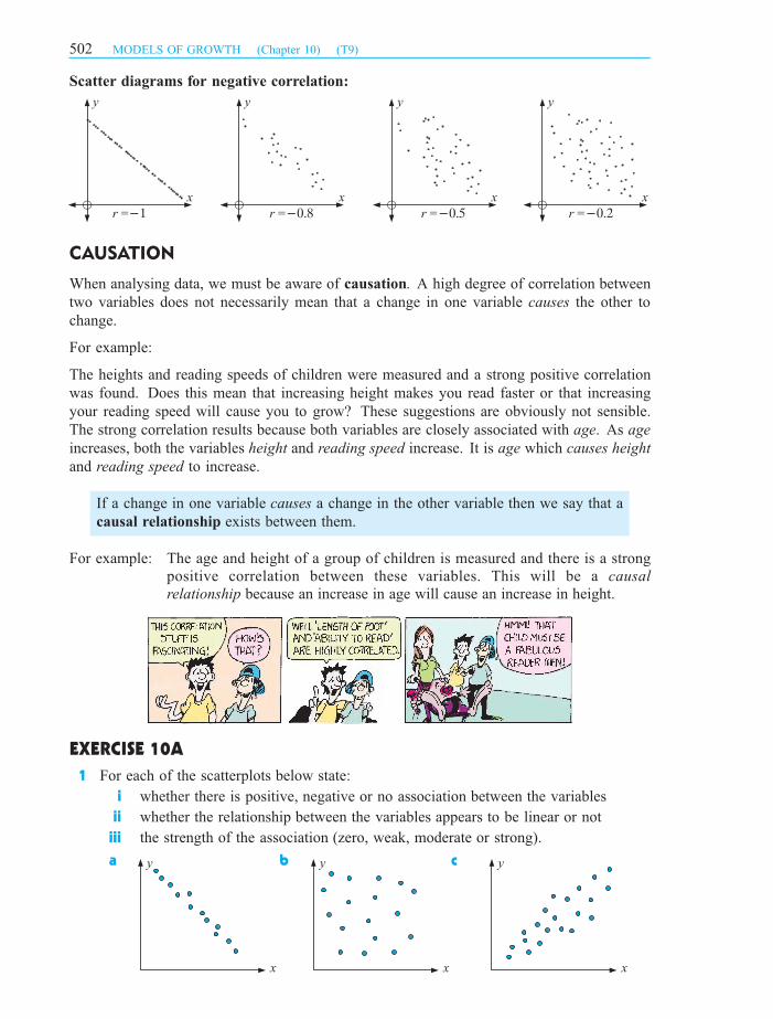
Scatter diagrams for negative correlation:
When analysing data, we must be aware of causation. A high degree of correlation between
two variables does not necessarily mean that a change in one variable causes the other to
change.
For example:
The heights and reading speeds of children were measured and a strong positive correlation
was found. Does this mean that increasing height makes you read faster or that increasing
your reading speed will cause you to grow? These suggestions are obviously not sensible.
The strong correlation results because both variables are closely associated with age. As age
increases, both the variables height and reading speed increase. It is age which causes height
and reading speed to increase.
If a change in one variable causes a change in the other variable then we say that a
causal relationship exists between them.
For example:
1 For each of the scatterplots below state:
i whether there is positive, negative or no association between the variables
ii whether the relationship between the variables appears to be linear or not
iii the strength of the association (zero, weak, moderate or strong).
a b c
y
x
���r =
y
x
���r =
y
x
���r =
y
x
�r =
CAUSATION
EXERCISE 10A
y
x
y
x
y
x
The age and height of a group of children is measured and there is a strongpositive correlation between these variables. This will be a
because an increase in age will cause an increase in height.causal
relationship
502 MODELS OF GROWTH (Chapter 10) (T9)
SA_11APPmagentacyan yellow black
0 05 5
25
25
75
75
50
50
95
95
100
100 0 05 5
25
25
75
75
50
50
95
95
100
100
Y:\HAESE\SA_11APP-2ed\SA11APP-2_10\502SA11APP-2_10.CDR Thursday, 6 September 2007 12:28:49 PM PETERDELL

y
x x
yy
x
d e f
2 Copy and complete the following:
a If the variables x and y are positively associated then as x increases, y .............
b If there is negative correlation between the variables m and n then as m increases,
n ..............
c If there is no association between two variables then the points on the scatterplot
appear to be ............. ...............
The statistician Pearson constructed a formula for calculating a correlation coefficient, which
he denoted r.
For a set of n data given as ordered pairs (x1, y1), (x2, y2), (x3, y3), ......, (xn, yn),
Pearson’s correlation coefficient r =
Pxy ¡ nxyp
(P
x2 ¡ nx2)(P
y2 ¡ ny2)
where x and y are the means of the x and y data respectively andP
means the
sum over all the data values.
To help describe the strength of asso-
ciation we calculate the coefficient of
determination (r2). This is simply the
square of the correlation coefficient (r)
and as such the direction of association
is eliminated.
Many texts vary on the advice they
give. We suggest using the table along-
side when describing the strength of
linear association.
value strength of association
r2 = 0 no correlation
0 < r2 < 0:25 very weak correlation
0:25 6 r2 < 0:50 weak correlation
0:50 6 r2 < 0:75 moderate correlation
0:75 6 r2 < 0:90 strong correlation
0:90 6 r2 < 1 very strong correlation
r2 = 1 perfect correlation
TWO VARIABLE ANALYSISB
PEARSON’S CORRELATION COEFFICIENT ( )r
THE COEFFICIENT OF DETERMINATION ( )r2
Pearson’s correlation coefficient, often called the , iscalculated directly from the data set.
linear correlation coefficient
MODELS OF GROWTH (Chapter 10) (T9) 503
SA_11APPmagentacyan yellow black
0 05 5
25
25
75
75
50
50
95
95
100
100 0 05 5
25
25
75
75
50
50
95
95
100
100
Y:\HAESE\SA_11APP-2ed\SA11APP-2_10\503SA11APP-2_10.CDR Thursday, 6 September 2007 12:28:56 PM PETERDELL

A chemical fertiliser company wishes
to determine the extent of correlation
between the ‘quantity of compound X
used’ and ‘lawn growth per day’.
Find and interpret the correlation
coefficient between the two variables.
Lawn Compound Lawn
X (gms) Growth (mm)
A 1 3B 2 3C 4 6D 5 8
x y x2 y2 xy
1 3 1 9 3
2 3 4 9 6
4 6 16 36 24
5 8 25 64 40
totals: 12 20 46 118 73
) x =
Px
n
=12
4
= 3
and y =
Py
n
=20
4
= 5
r =
Pxy ¡ nx yp
(P
x2 ¡ nx2)(P
y2 ¡ ny2)=
73 ¡ 4 £ 3 £ 5p(46 ¡ 4 £ 32)(118¡ 4 £ 52)
=13p
10 £ 18
+ 0:969 and so r2 + 0:939
There is a very strong positive correlation between the quantity of compound X
used and lawn growth.
This suggests that the more of compound X used, the greater the lawn growth
per day. However, the small amount of data may provide a misleading result.
1 Consider the three graphs given below:
A B C
Clearly: A shows perfect positive linear correlation
B shows perfect negative linear correlation
C shows no correlation.
a For each set of points, find r using r =
Pxy ¡ nxyp
(P
x2 ¡ nx2)(P
y2 ¡ ny2)
b Comment on the values of r for each graph.
Self TutorExample 2
EXERCISE 10B.1
x
y
( )����,
( )����,
( )����,
( )���,x
y
1
2
1 2 3
3
x
y
( )����,
( )����,
( )����,
( )���,
504 MODELS OF GROWTH (Chapter 10) (T9)
SA_11APPmagentacyan yellow black
0 05 5
25
25
75
75
50
50
95
95
100
100 0 05 5
25
25
75
75
50
50
95
95
100
100
Y:\HAESE\SA_11APP-2ed\SA11APP-2_10\504SA11APP-2_10.CDR Thursday, 6 September 2007 12:29:01 PM PETERDELL

2 Determine Pearson’s correlation coefficient for the variables in the following cases,
commenting on the result of each calculation.
a Length and Weight of mice:Length (cm) 5 6 7 8
Weight (g) 14 22 26 30
b Weedicide concentration and
Number of weeds surviving:Weedicide (mg/L) 5 10 15 20
Number of weeds surviving 43 25 10 2
We will now take the chemical fertiliser problem in Example 2 a little further.
We know that there is a very strong positive correlation between the two variables.
We should therefore be able to find a
linear function, often called a line of
best fit, to closely model the relation-
ship between length and mass. We
could fit a line ‘by eye’, as shown
alongside.
However, different people will use
different lines.
So, how do we find the line of best fit
mathematically?
Statisticians invented a method where the best line results. The process is minimisation of
the sum of the squares of the residuals.
The mathematics behind this method is generally
established in university mathematics courses,
but in brief what happens is that we find ver-
tical distances or residuals to the line of best fit:
d1, d2, d3, .... etc.
We then add the squares of the residuals,
i.e., d 21 + d 2
2 + d 23 + ::::::
The least squares regression line is the one
which makes this sum as small as possible.
Click on the icon and use trial and error to try to find the least
The least squares line has equation y = mx+ c where m =
Pxy ¡ 1
n(P
x)(P
y)
(P
x2) ¡ 1
n(P
x)2
and c = y ¡mx
LEAST SQUARES ‘LINE OF BEST FIT’
0
2
4
6
8
10
0 1 2 3 4 5 6 7 8 9 10
line of best fit (by eye)
Growth ( mm)y
Compound ( g)X x
d1
d2 d3
d4
d5
y
x
COMPUTER
DEMO
MODELS OF GROWTH (Chapter 10) (T9) 505
squares line of best fit for the data sets given.
SA_11APPmagentacyan yellow black
0 05 5
25
25
75
75
50
50
95
95
100
100 0 05 5
25
25
75
75
50
50
95
95
100
100
Y:\HAESE\SA_11APP-2ed\SA11APP-2_10\505SA11APP-2_10.CDR Friday, 7 September 2007 10:55:14 AM PETERDELL

Once the line of best fit is determined and you have its equation then you can use it to predict
other values that the experiment did not reveal.
For the chemical fertiliser data of Example 2, find the least squares ‘line of best fit’.
x y xy x2
1 3 3 12 3 6 44 6 24 165 8 40 25P12 20 73 46
x =
Px
n=
12
4= 3, y =
Py
n=
20
4= 5
m =
Pxy ¡ 1
n(P
x)(P
y)
(P
x2) ¡ 1
n(P
x)2
) m =73 ¡ 1
4£ 12 £ 20
46 ¡ 1
4£ 122
= 1:3
and c = y ¡mx = 5 ¡ 1:3 £ 3 = 1:1
) line of best fit is y = 1:3x + 1:1
With many points and much more complicated numbers, the task of finding r, r2, m and c
can be very tedious using the given formulae.
We use technology to ease the work load.
Self TutorExample 3
USING A COMPUTER PACKAGE
COMPUTER
PACKAGEClick on the icon to obtain the package. Enter thedata and observe how the correlation coefficient, coefficient of determination,and line of best fit are automatically calculated.
Two Variable Analysis
506 MODELS OF GROWTH (Chapter 10) (T9)
SA_11APPmagentacyan yellow black
0 05 5
25
25
75
75
50
50
95
95
100
100 0 05 5
25
25
75
75
50
50
95
95
100
100
Y:\HAESE\SA_11APP-2ed\SA11APP-2_10\506SA11APP-2_10.CDR Thursday, 6 September 2007 12:29:12 PM PETERDELL

Returning to the chemical fertiliser example we can use the line of best fit y = 1:3x + 1:1to predict the lawn growth per day for other quantities of compound x.
If we substitute a quantity in between the smallest and largest quantities in the experiment,
we say we are interpolating (in between the poles).
If we predict length values for quantities outside the smallest and largest quantities in the
experiment, we say we are extrapolating (outside the poles).
The accuracy of an interpolation depends on
how linear the original data was. This can be
gauged by determining the correlation coeffi-
cient and ensuring that the data is randomly
scattered around the line of best fit.
The accuracy of an extrapolation depends not
only on ‘how linear’ the original data was, but
also on the assumption that the linear trend
will continue past the poles.
The validity of this assumption depends
greatly on the situation under investigation.
In the chemical fertiliser example, there is
a point where the addition of more fertiliser
will no longer be beneficial, and may even be
harmful, to the lawn’s growth.
USING A GRAPHICS CALCULATOR
INTERPOLATION AND EXTRAPOLATION
lowerpole
upperpole
line ofbest fit
y
x
interpolationextrapolation extrapolation
Using a Casio fx-9860G
Select STAT from the main menu, then key
the x values into List 1 and the y values
into List 2.
To find the line of best fit, press (¤)
if the GRPH icon is not in the bottom left
corner of the screen, then press
(CALC) (REG) (X).
The line of best fit y = 1.3x + 1.1 is
given.
Using a Texas Instruments TI-83
Press 1 to enter the list editor, then
key the x values into L1 and the y values
into L2.
To find the line of best fit, press
4, which selects 4:LinReg(ax+b) from the
CALC menu.
Press 1 (L1) , 2 (L2)
ENTER to display the result. The line of
best fit is given as y = 1.3x + 1.1
MODELS OF GROWTH (Chapter 10) (T9) 507
SA_11APPmagentacyan yellow black
0 05 5
25
25
75
75
50
50
95
95
100
100 0 05 5
25
25
75
75
50
50
95
95
100
100
Y:\HAESE\SA_11APP-2ed\SA11APP-2_10\507SA11APP-2_10.CDR Friday, 14 September 2007 10:44:50 AM DAVID3

An example could be the world record for the long jump
prior to the Mexico City Olympic Games of 1968. A
steady regular increase in the World record over the pre-
vious 30 years had been recorded. However, due to the
high altitude and a perfect jump, the USA competitor
Bob Beamon shattered the record by a huge amount,
not in keeping with previous increases.
In general, interpolation between the poles is reliable, but extrapolation outside the poles can
be unreliable.
1 Tomatoes are sprayed with a pesticide-fertiliser mix. The figures below give the yield of
tomatoes per bush for various spray concentrations.
Spray concentration (x mL/L) 3 5 6 8 9 11
Yield of tomatoes per bush (y) 67 90 103 120 124 150
a Draw a scatterplot for this data.
b Determine the r and r2 values.
c Describe the association between yield and spray
concentration.
d Find the least squares line of best fit for the data.
e Predict the yield when the spray concentration is
7 mL/L. How reliable is this result?
f Predict the yield when the spray concentration is
15 mL/L. How reliable is this result?
2 The following data shows the annual cherry yield and number of frosts data for a cherry
growing farm over a 7 year period.
Number of frosts (x) 27 23 7 37 32 14 16
Cherry yield (y tonnes) 5:6 4:8 3:1 7:2 6:1 3:7 3:8
a Draw a scatterplot for this data.
b Determine the r and r2 values.
c Describe the association between the cherry yield
and the number of frosts.
d Find the least squares line of best fit for the data.
e Predict the yield when the number of frosts is 20.
How reliable is this result?
f Predict the yield when the number of frosts is 45.
How reliable is this result?
CARE MUST BE TAKEN WHEN EXTRAPOLATING
EXERCISE 10B.2
508 MODELS OF GROWTH (Chapter 10) (T9)
SA_11APPmagentacyan yellow black
0 05 5
25
25
75
75
50
50
95
95
100
100 0 05 5
25
25
75
75
50
50
95
95
100
100
Y:\HAESE\SA_11APP-2ed\SA11APP-2_10\508SA11APP-2_10.CDR Thursday, 6 September 2007 12:29:23 PM PETERDELL

3 The following data shows the top speed of a Formula One racing car when it is filled
with various quantities of petrol.
Petrol quantity (xL) 50 37 18 85 27 102
Top speed (y km/h) 315 319 323 311 321 308
a Draw a scatterplot for this data.
b Determine the r and r2 values.
c Describe the association between the top speed and the petrol quantity.
d Find the least squares line of best fit for the data.
e If the capacity of the petrol tank is 120 litres, predict the top speed of the car when
the tank is i full ii half full iii nearly empty.
f Which of the predictions in e is likely to be most accurate?
4 The following table gives the value of a television set at various times t years after it
was bought.
Time (t years) 2 5 7 10 12
Value (V dollars) 900 745 655 500 405
a Draw a scatterplot for this data.
b Determine the r and r2 values.
c Describe the association between value and time.
d Find the least squares line of best fit of the data.
e Estimate the value of the TV set 15 years after it was bought. How reliable is this
result?
f Is it reasonable to assume that the linear trend displayed by the data will continue
indefinitely? Explain.
Before examining exponential functions and their properties we will revise the laws of indices.
We are already familiar with index or exponential notation. For example, 8 = 2£2£2 = 23
In general, an = a£ a£ a£ a£ ::::£ a| {z }n factors
where n is a positive integer.
Recall that: ² 34 £ 32 = (3 £ 3 £ 3 £ 3) £ (3 £ 3) = 34+2 = 36
as we have six 3s multiplied together.
² 35
32=
3 £ 3 £ 3 £ 3 £ 3
3 £ 3= 35¡2 = 33
² (33)2 = 33 £ 33 = 33+3 = 36
LAWS OF INDICES (Revision)C
i.e., 8 = 23 index, power or exponent
base number
MODELS OF GROWTH (Chapter 10) (T9) 509
SA_11APPmagentacyan yellow black
0 05 5
25
25
75
75
50
50
95
95
100
100 0 05 5
25
25
75
75
50
50
95
95
100
100
Y:\HAESE\SA_11APP-2ed\SA11APP-2_10\509SA11APP-2_10.CDR Thursday, 6 September 2007 12:29:29 PM PETERDELL

So, to get from 34 £ 32 to 36, we add indices
35
32to 33, we subtract indices
(33)2 to 36 we multiply indices
² am £ an = am+n
² am
an= am¡n
² (am )n = amn
Notice also that 23 £ 20 = 23+0 = 23, so 20 must be 1.
In fact, a0 = 1 for all a 6= 0
The laws for expanding powers of products and quotients are:
(ab)n = anbn and
µa
b
¶n
=an
bn(b 6= 0)
Finally notice that a¡n £ an = a¡n+n = a0 = 1
Thus, a¡n and an are reciprocals, and a¡n =1
anfor all a 6= 0:
1 Simplify mentally:
a a2 £ a7 b m3 £m4 c d7 £ d d k8 £ k3
en4
n2f
m7
m3g
g6
g4h
s41
s17
i (a5)2 j (m3)4 k (n4)5 l (p7)3
2 Remove the brackets using an index law:
a (ab)5 b (mn)4 c (2xy)2 d (3ab2)3
e³an
´4f
³x2
´4g
µ3
y
¶4
h
µ2a
b
¶4
Examples like these helpus establish that:
EXERCISE 10C
Write as powers of 2: a 16 b 1
16c 1
a 16
= 2 £ 2 £ 2 £ 2
= 24
b 1
16
=1
24
= 2¡4
c 1
= 20
Self TutorExample 4
510 MODELS OF GROWTH (Chapter 10) (T9)
SA_11APPmagentacyan yellow black
0 05 5
25
25
75
75
50
50
95
95
100
100 0 05 5
25
25
75
75
50
50
95
95
100
100
Y:\HAESE\SA_11APP-2ed\SA11APP-2_10\510SA11APP-2_10.CDR Thursday, 6 September 2007 12:29:34 PM PETERDELL

3 Write as powers of 2:
a 4
g 2
4 Write as powers of 3:
a 9
f 1
32
l 1
128
f 1
3
g 81
b 1
4
h 1
2
b 1
9
h 1
81
c 8
i 64
c 27
i 1
d 1
8
j 1
64
d 1
27
j 243
e 32
k 128
e 3
k 1
243
5 Write as a single power of 2:
a 2 £ 2a
f2c
4
6 Write as a single power of 3:
a 9 £ 3p
f3y
3
b 4 £ 2b
g2m
2¡m
b 27a
g3
3y
c 8 £ 2t
h4
21¡n
c 3 £ 9n
h9
27t
d (2x+1)2
i2x+1
2x
d 27 £ 3d
i9a
31¡a
e (21¡n)¡1
j4x
21¡x
e 9 £ 27t
j9n+1
32n¡1
Write without negative indices: a (3x)¡2 b³ a
2b
´¡3
a (3x)¡2
=
µ3x
1
¶¡2
=
µ1
3x
¶2
=1
9x2
b³ a
2b
´¡3
=
µ2b
a
¶3
=23b3
a3
=8b3
a3
Write as a single power of 2: a 4 £ 2n b2m
8
a 4 £ 2n
= 22 £ 2n
= 22+n
b2m
8
=2m
23
= 2m¡3
Self TutorExample 5
Self TutorExample 6 We can changea negative
index into itspositive by
reciprocatingthe contents ofthe brackets.
MODELS OF GROWTH (Chapter 10) (T9) 511
SA_11APPmagentacyan yellow black
0 05 5
25
25
75
75
50
50
95
95
100
100 0 05 5
25
25
75
75
50
50
95
95
100
100
Y:\HAESE\SA_11APP-2ed\SA11APP-2_10\511SA11APP-2_10.CDR Thursday, 6 September 2007 12:29:39 PM PETERDELL
7 Write without negative indices:
a a¡4 b (ab)¡2 c³ab
´¡1
d (2x)¡3
e³x
2
´¡2
f (4b)¡1 g
µ3m
n
¶¡1
h
µ2a
b
¶¡2
Since a12 £ a
12 = a
12+ 1
2 = a1 = a, ffor index laws to be obeyedgand
pa£p
a = a also, then
a1
2 =pa. fby direct comparisong
Likewise a13 £ a
13 £ a
13 = a1 = a,
compared with 3pa£ 3
pa£ 3
pa = a
suggests a1
3 = 3pa.
Thus in general, a1
n = npa. f n
pa reads “the nth root of a”g
Notice also that a23 £ a
23 £ a
23 = a2
)
³a
23
´3= a2 fusing (am)n = amn g
) a23 =
3pa2:
In general, amn = n
pam .
Write as a single power of 2: a3p
2 b1p2
c5p
4
a3p
2
= 213
b1p2
=1
212
= 2¡
12
c5p
4
= (22)15
= 22£ 1
5
= 225
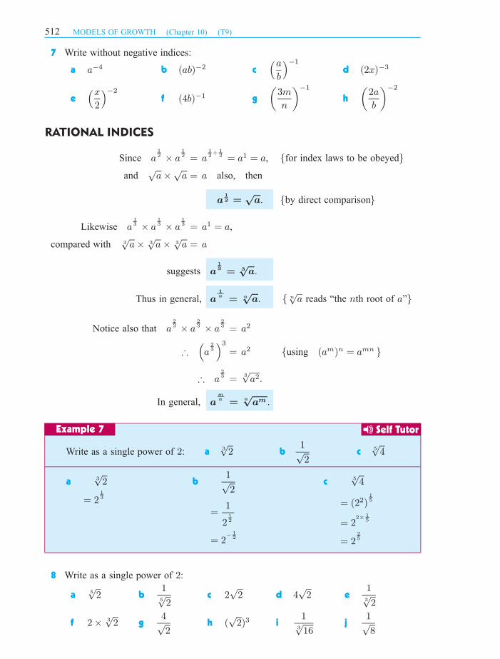
8 Write as a single power of 2:
a5p
2 b15p
2c 2
p2 d 4
p2 e
13p
2
f 2 £ 3p
2 g4p2
h (p
2)3 i1
3p
16j
1p8
RATIONAL INDICES
Self TutorExample 7
512 MODELS OF GROWTH (Chapter 10) (T9)
SA_11APPmagentacyan yellow black
0 05 5
25
25
75
75
50
50
95
95
100
100 0 05 5
25
25
75
75
50
50
95
95
100
100
Y:\HAESE\SA_11APP-2ed\SA11APP-2_10\512SA11APP-2_10.CDR Thursday, 6 September 2007 12:29:44 PM PETERDELL

9 Write as a single power of 3:
a3p
3 b13p
3c
4p
3 d 3p
3 e1
9p
3
Use your calculator to evaluate a 275 b 5
p4
Calculator: Answer:
For 275 so press: 2:639 015
5p
4 = 415 so press: 4 1 5 1:319 507
10 Use your calculator to find:
a 334 b 2
78 c 2
¡13 d 4
¡35
ep
9 f4p
8 g5p
27 h13p
7
Split these fractions into separate terms with no fractions:
a2x2 + 1
xb
x3 + x2 ¡ 2x + 3
x2
a2x2 + 1
x
=2x2
x+
1
x
= 2x + x¡1
bx3 + x2 ¡ 2x + 3
x2
=x3
x2+
x2
x2¡ 2x
x2+
3
x2
= x + 1 ¡ 2x¡1 + 3x¡2
11 Split these fractions into separate terms with no fractions:
ax + 3
xb
x2 ¡ 2
xc
x2 + 3x ¡ 4
x
dx2 + 5x
x2e
x3 + 2x2 ¡ 6
x2f
x3 + 2x2 ¡ 3x + 5
x2
gx4 + x2 + 1
x3h
x5 + 3x2 ¡ 5
x3i
2x4 + 3x2 ¡ 6x + 5
x3
jx2 + x¡1 + 5
x¡1k
x + 2x2 ¡ 6
x¡2l
x2 + 3x ¡ 4x¡1
x¡3
Self TutorExample 9
Self TutorExample 8
2 7 5^ ( ÷ ) ENTER
^ ( ÷ ) ENTER
MODELS OF GROWTH (Chapter 10) (T9) 513
a
b
SA_11APPmagentacyan yellow black
0 05 5
25
25
75
75
50
50
95
95
100
100 0 05 5
25
25
75
75
50
50
95
95
100
100
Y:\HAESE\SA_11APP-2ed\SA11APP-2_10\513SA11APP-2_10.CDR Friday, 28 September 2007 9:29:37 AM DAVID3

Without using a calculator, write in simplest rational form: a 843 b 27
¡23
a 843 b 27
¡23
= (23)43 = (33)
¡23
= 23£ 4
3 f(am)n = amng = 33£¡
23
= 24 = 3¡2
= 16 = 1
9
12 Without using a calculator, write in simplest rational form:
a 432 b 8
53 c 16
34 d 25
32 e 32
25
f 4¡
12 g 9
¡32 h 8
¡43 i 27
¡43 j 125
¡23
The simplest exponential function has the form y = ax where a > 0, a 6= 1.
For example, y = 2x is an exponential function.
Table of values:x ¡3 ¡2 ¡1 0 1 2 3
y 1
8
1
4
1
21 2 4 8
We notice that for x = ¡10, y = 2¡10 + 0:001
and when x = ¡50, y = 2¡50 + 8:88 £ 10¡16
So, it appears that as x becomes large and negative, the
graph of y = 2x approaches the x-axis from above it.
We say that y = 2x is ‘asymptotic to the x-axis’, or
‘y = 0 is a horizontal asymptote’.
Self TutorExample 10
GRAPHS OF EXPONENTIALSD
INVESTIGATION 1 EXPONENTIAL GRAPHS
1 a On the same set of axes, use a graphing package or graphics calculator to graph
the following functions: y = 2x, y = 3x, y = 10x, y = (1:3)x.
b The functions in a are all members of the family y = bx:
i What effect does changing b values have on the shape of the graph?
ii What is the y-intercept of each graph?
iii What is the horizontal asymptote of each graph?
x
y
1
1
� � 2 3
2
4
6
8
y = 2x
What to do:
We will investigate families ofexponential functions.
TI
C
GRAPHING
PACKAGE
514 MODELS OF GROWTH (Chapter 10) (T9)
SA_11APPmagentacyan yellow black
0 05 5
25
25
75
75
50
50
95
95
100
100 0 05 5
25
25
75
75
50
50
95
95
100
100
Y:\HAESE\SA_11APP-2ed\SA11APP-2_10\514SA11APP-2_10.CDR Thursday, 6 September 2007 12:29:54 PM PETERDELL

2 a On the same set of axes, use technology to graph the following functions:
y = (0:5)x, y = (0:8)x, y = (0:96)x.
b The functions in a are all members of the family y = ax, 0 < a < 1.
i What effect does changing a have on the shape of the graph?
ii What is the y-intercept of each graph?
iii What value is y approaching as x is large and negative?
From your investigation you should have discovered that:
1 Given the graph of y = 2x we can find
approximate values of 2x for various
values of x.
For example:
² 21:8 + 3:5 (see point A)
² 22:3 + 5 (see point B)
Use the graph to determine approximate
values of:
a 212 (=
p2) b 20:8
c 21:5 d 2¡1:6
2
a y = 2x and y = 2x ¡ 2 b y = 2x and y = 2¡x
c y = 2x and y = 2x¡2 d y = 2x and y = 2 £ 2x
3 The graph of y = 3x is given alongside. Draw free-
hand sketches of the following pairs of graphs:
a y = 3x and y = 3¡x
b y = 3x and y = 3x + 1
c y = 3x and y = ¡3x
d y = 3x and y = 3x¡1
y
x
1
ƒ( )x ���x
GRAPHING
PACKAGE
for the general exponential function y = ax
² a controls how steeply the graph increases or decreases
² the graphs are all asymptotic to the x-axis (i.e., approach it)
² ²if thegraph isincreasingfor all
a>
x
� �1 ifthe graph isdecreasing forall
0 1� � � �<a<
x
EXERCISE 10D
Draw freehand sketches of the following pairs of graphsbased on your observations from the previous investigation.
MODELS OF GROWTH (Chapter 10) (T9) 515
11
1111�� 22
22
33
44
yy
xx
y = 2x
y = 2x
AA
1.81.8
3.53.5
BB55
SA_11APPmagentacyan yellow black
0 05 5
25
25
75
75
50
50
95
95
100
100 0 05 5
25
25
75
75
50
50
95
95
100
100
Y:\HAESE\SA_11APP-2ed\SA11APP-2_10\515SA11APP-2_10.CDR Friday, 14 September 2007 4:59:55 PM DAVID3

For the general exponential function
y = bkx + c, y = c is the horizontal asymptote.
We can actually obtain reasonably accurate sketch
graphs of exponential functions using
² the horizontal asymptote
² the y-intercept
² two other points, say when x = 2, x = ¡2
Sketch the graph of y = 2¡x ¡ 3:
For y = 2¡x ¡ 3the horizontal asymptote is y = ¡3
when x = 0, y = 20 ¡ 3
= 1 ¡ 3
= ¡2
) the y-intercept is ¡2
when x = 2, y = 2¡2 ¡ 3
= 1
4¡ 3
= ¡23
4
when x = ¡2, y = 22 ¡ 3
= 4 ¡ 3
= 1
4 Sketch the graphs of:
a y = 2x + 1 b y = 2 ¡ 2x c y = 2¡x + 3 d y = 3 ¡ 2¡x
In this section we will examine situations where quantities are increasing or decreasing
exponentially. We describe these situations as exponential growth and decay.
Populations of animals, people, bacteria, and so on, usually grow in an exponential way.
Radioactive substances and items that depreciate usually decay exponentially.
y
x
��
y��
y��� ���x
2
HORIZONTAL ASYMPTOTES
All exponentialgraphs aresimilar in
shape and havea horizontalasymptote.
Self TutorExample 11
GROWTH AND DECAYE
516 MODELS OF GROWTH (Chapter 10) (T9)
SA_11APPmagentacyan yellow black
0 05 5
25
25
75
75
50
50
95
95
100
100 0 05 5
25
25
75
75
50
50
95
95
100
100
Y:\HAESE\SA_11APP-2ed\SA11APP-2_10\516SA11APP-2_10.CDR Thursday, 6 September 2007 12:30:07 PM PETERDELL

So, if Pn is the population after n weeks, then:
P0 = 100 fthe original populationgP1 = P0 £ 1:2 = 100 £ 1:2
P2 = P1 £ 1:2 = 100 £ (1:2)2
P3 = P2 £ 1:2 = 100 £ (1:2)3
...
etc, and from this pattern we see that Pn = 100 £ (1:2)n:
An entomologist monitoring a grasshopper plague notices that the area affected
by the grasshoppers is given by An = 1000£ 20:2n hectares, where n is the
number of weeks after the initial observation.
a Find the original affected area.
b Find the affected area after i 5 weeks ii 10 weeks.
c Find the affected area after 12 weeks.
d Draw the graph of An against n.
a A0 = 1000 £ 20
= 1000 £ 1
= 1000
) original area was 1000 ha.
b i A5 = 1000 £ 21
= 2000
) affected area is 2000 ha.
ii A10 = 1000 £ 22
= 4000
) affected area is 4000 ha.
c A12 = 1000£ 20:2£12
= 1000£ 22:4 fPress: 1000 2 2:4 g+ 5278
) after 12 weeks, the area affected is about 5300 ha.
d
BIOLOGICAL GROWTH
Consider a population of mice which underfavourable conditions is increasing by each week.To increase a quantity by , we multiply it by
or .
10020%
20%120% 1 2:
Self TutorExample 12
×
b i
a
b ii
c
1412108642
6000
4000
2000
A (ha)
n (weeks)
^ ENTER
100
200
300
400
P
n (weeks)
n
1 2 3 4 5 6
MODELS OF GROWTH (Chapter 10) (T9) 517
SA_11APPmagentacyan yellow black
0 05 5
25
25
75
75
50
50
95
95
100
100 0 05 5
25
25
75
75
50
50
95
95
100
100
Y:\HAESE\SA_11APP-2ed\SA11APP-2_10\517SA11APP-2_10.CDR Thursday, 6 September 2007 12:30:12 PM PETERDELL

1 The weight of bacteria in a culture t hours after establishment
is given by Wt = 100 £ 20:1t grams. Find:
a the initial weight
b the weight after i 4 hours ii 10 hours iii 24 hours.
c Sketch the graph of Wt against t using only results from a and b.
d Use technology to graph Y1 = 100£ 20:1X and check your answers to a, b and c.
2 A breeding program to ensure the survival of
pygmy possums was established with an ini-
tial population of 50 (25 pairs). From a previ-
ous program, the expected population Pn in n
years’ time is given by Pn = P0 £ 20:3n .
a What is the value of P0?
b What is the expected population after:
i 2 years ii 5 years iii 10 years?
c Sketch the graph of Pn against n using
only a and b.
d Use technology to graph Y1 = 50 £ 20:3X and use it to check your answers in b.
3 The speed Vt of a chemical reaction is given by Vt = V0 £ 20:05t where t is the
temperature in oC. Find:
a the speed at 0oC
b the speed at 20oC
c the percentage increase in speed at 20oC compared with the speed at 0oC.
Now consider a radioactive substance of original
weight 20 grams which decays (reduces) by 5% each
year. The multiplier is now 95% or 0:95.
So, if Wn is the weight after n years, then:
W0 = 20 grams
W1 = W0 £ 0:95 = 20 £ 0:95 grams
W2 = W1 £ 0:95 = 20 £ (0:95)2 grams
W3 = W2 £ 0:95 = 20 £ (0:95)3 grams... etc.
and from this we see that Wn = 20 £ (0:95)n.
If the original weight W0 is unknown then JM
Wn = W0 £ (0:95)n.
EXERCISE 10E
GRAPHING
PACKAGE
DECAY
10 20
25
20
15
10
5
Wn (grams)
n (years)
518 MODELS OF GROWTH (Chapter 10) (T9)
SA_11APPmagentacyan yellow black
0 05 5
25
25
75
75
50
50
95
95
100
100 0 05 5
25
25
75
75
50
50
95
95
100
100
Y:\HAESE\SA_11APP-2ed\SA11APP-2_10\518SA11APP-2_10.CDR Friday, 7 September 2007 10:56:06 AM PETERDELL

The weight of radioactive material remaining after t years is given by
Wt = 11:7 £ 2¡0:0067t grams.
a Find the original weight.
b Find the weight after i 10 years ii 100 years iii 1000 years.
c Graph Wt against t using a and b only.
Wt = 11:7 £ 2¡0:0067t
a When t = 0, W0 = 11:7 £ 20 = 11:7 grams
b i W10
= 11:7 £ 2¡0:067
+ 11:17 g
c
ii W100
= 11:7 £ 2¡0:67
+ 7:35 g
iii W1000
= 11:7 £ 2¡6:7
+ 0:11 g
4 The temperature Tt of a liquid which has been placed in a refrigerator is given by
Tt = 100 £ 2¡0:02t degrees Celsius, where t is the time in minutes. Find:
a the initial temperature
b the temperature after i 15 min ii 20 min iii 78 min.
c Sketch the graph of Tt against t using a and b only.
5 The weight Wt of radioactive substance remaining after t years is given by
Wt = 1000 £ 2¡0:03t grams. Find:
a the initial weight
b the weight after i 10 years ii 100 years iii 1000 years.
c Graph Wt against t using a and b only.
6 The weight Wt of radioactive uranium remaining after t years is given by the formula
Wt = 25 £ 2¡0:0002t grams, t > 0. Find:
a the original weight b the percentage weight loss after 2000 years.
7 The current It flowing in a transistor radio t seconds after it is switched off is given by
It = 35 £ 2¡0:02t amps. Find:
a the initial current
b the current after 1 second
c the percentage change in current after 1 second
d I50 and I100 and hence sketch the graph of It against t.
Self TutorExample 13
12001000800600400200
12
10
8
6
4
2
(10' 11"17)
(100' 7"35)
(1000' 0"11)
Wt (grams)
t (years)
11.7
MODELS OF GROWTH (Chapter 10) (T9) 519
SA_11APPmagentacyan yellow black
0 05 5
25
25
75
75
50
50
95
95
100
100 0 05 5
25
25
75
75
50
50
95
95
100
100
Y:\HAESE\SA_11APP-2ed\SA11APP-2_10\519SA11APP-2_10.CDR Thursday, 6 September 2007 12:30:23 PM PETERDELL
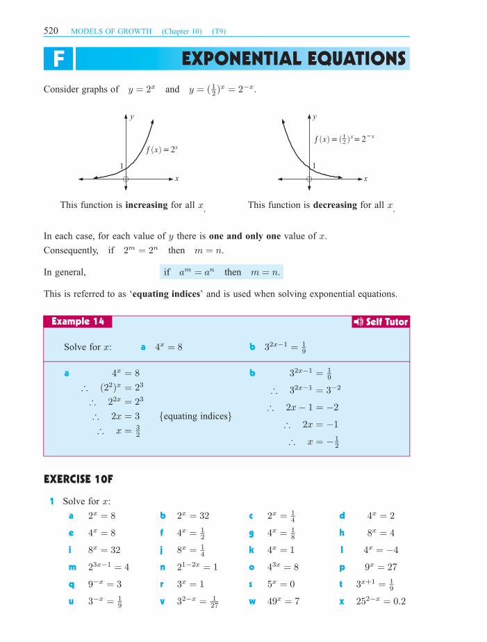
Consider graphs of y = 2x and y = (12)x = 2¡x:
This function is increasing for all x. This function is decreasing for all x.
In each case, for each value of y there is one and only one value of x.
Consequently, if 2m = 2n then m = n.
In general, if am = an then m = n.
This is referred to as ‘equating indices’ and is used when solving exponential equations.
Solve for x: a 4x = 8 b 32x¡1 = 1
9
a 4x = 8
) (22)x = 23
) 22x = 23
) 2x = 3 fequating indicesg) x = 3
2
b 32x¡1 = 1
9
) 32x¡1 = 3¡2
) 2x¡ 1 = ¡2
) 2x = ¡1
) x = ¡1
2
1 Solve for x:
a 2x = 8 b 2x = 32 c 2x = 1
4d 4x = 2
e 4x = 8 f 4x = 1
2g 4x = 1
8h 8x = 4
i 8x = 32 j 8x = 1
4k 4x = 1 l 4x = ¡4
m 23x¡1 = 4 n 21¡2x = 1 o 43x = 8 p 9x = 27
q 9¡x = 3 r 3x = 1 s 5x = 0 t 3x+1 = 1
9
u 3¡x = 1
9v 32¡x = 1
27w 49x = 7 x 252¡x = 0:2
EXPONENTIAL EQUATIONSF
y
x
1
� ���( )x x
y
x
1
� �� � ��( ) (Qw_ )x x x�� �
Self TutorExample 14
EXERCISE 10F
520 MODELS OF GROWTH (Chapter 10) (T9)
SA_11APPmagentacyan yellow black
0 05 5
25
25
75
75
50
50
95
95
100
100 0 05 5
25
25
75
75
50
50
95
95
100
100
Y:\HAESE\SA_11APP-2ed\SA11APP-2_10\520SA11APP-2_10.CDR Thursday, 6 September 2007 12:30:28 PM PETERDELL

Solve for x: a 5 £ 2x = 40 b 18 £ 3x = 2
a 5 £ 2x = 40
) 2x = 8 f¥ both sides by 5g) 2x = 23
) x = 3 fequating indicesg
b 18 £ 3x = 2
) 3x = 1
9f¥ by 18g
) 3x = 3¡2
) x = ¡2
2 Solve for x:
a 3 £ 2x = 24 b 7 £ 2x = 56 c 3 £ 2x+1 = 24
d 12 £ 3¡x = 4
3e 4 £ (1
3)x = 36 f 5 £ (1
2)x = 20
Often it is not possible to select a common base and then equate indices.
For example, in 2x = 5. We use technology to solve these equations.
Self TutorExample 15
Using a Casio fx-9860G
Select EQUA from the main menu, then
press (Solver).
Enter the equation by pressing 2 ^. (=) 5 .
Make sure the cursor is on the guess for X,
then press (SOLV) to solve the
equation.
The solution x + 2:32 is given.
Using a Texas Instruments TI-83
Press 0 to select 0:Solver… Press
to delete the previous equation.
We must rearrange the equation so that one
side is equal to zero, so the equation
becomes
Enter this by pressing 2 ^ 5
ENTER .
Make sure the cursor is on the guess for X,
then press ENTER (SOLVE) to
solve the equation.
2x ¡ 5 = 0.
The solution x + 2:32 is given.
MODELS OF GROWTH (Chapter 10) (T9) 521
SA_11APPmagentacyan yellow black
0 05 5
25
25
75
75
50
50
95
95
100
100 0 05 5
25
25
75
75
50
50
95
95
100
100
Y:\HAESE\SA_11APP-2ed\SA11APP-2_10\521SA11APP-2_10.CDR Friday, 14 September 2007 10:45:41 AM DAVID3

3 Solve for x, correct to 3 s.f.:
a 2x = 100 b 3x = 0:067 c 5x = 2578
d (1:2)x = 14:89 e (0:97)x = 0:032 f 2¡x = 0:0075
g 3¡x = 0:000 842 h 2x+2 = 23:96 i 100 £ 2x = 602:8
j 200 £ 3x = 10:8 k 50:8 £ 5x = 1 l 0:0873 £ 2x = 14
4 The weight Wt of bacteria in a culture t hours after establishment is given by
Wt = 20 £ 20:15t grams. Find the time for the weight of the culture to reach:
a 30 grams b 100 grams.
5 The temperature T of a liquid which has been placed in a refrigerator is given by
T = 100 £ 2¡0:03t degrees Celsius, where t is the time in minutes. Find the time
required for the temperature to reach:
a 25oC b 1oC.
6 The weight Wt of radioactive substance remaining after t years is given by
Wt = 1000 £ 2¡0:04t grams. Find the time taken for the weight to:
a halve b reach 20 grams c reach 1% of its original value.
The weight of radioactive material remaining after t years is given by
W = 30 £ 2¡0:001t grams. Find:
a the original weight
b how long it would take for the material to decay to 10 grams
c how long it would take for the material to decay to the ‘safe level’ of 1%of its original value.
a When t = 0, W = 30 £ 20 = 30
So, 30 g is the original weight.
b For W = 10
30 £ 2¡0:001t = 10
) 2¡0:001t = 1
3
) t + 1584 fusing technologyg) it would take about 1580 years.
c For W = 1% of the original weight
30 £ 2¡0:001t = 1
100£ 30
) 2¡0:001t = 0:01
) t + 6644 fusing technologyg) it would take about 6640 years.
Self TutorExample 16
522 MODELS OF GROWTH (Chapter 10) (T9)
SA_11APPmagentacyan yellow black
0 05 5
25
25
75
75
50
50
95
95
100
100 0 05 5
25
25
75
75
50
50
95
95
100
100
Y:\HAESE\SA_11APP-2ed\SA11APP-2_10\522SA11APP-2_10.CDR Thursday, 6 September 2007 12:30:38 PM PETERDELL

7 The weight W of radioactive uranium remaining after t years is given by the formula
W = 1200 £ 2¡0:0002t grams, t > 0. Find the time taken for the original weight to
fall to:
a 25% of its original value b 0:1% of its original value.
8 A man jumps from the basket of a stationary hot
air balloon. His speed of descent is given by
V = 50(1 ¡ 2¡0:2t) m/s where t is the time in
seconds.
Find the time taken for his speed to reach 40 m/s.
9 Hot cooking oil is placed in a freezer and
its temperature after m minutes is given by
Tm = (225 £ 2¡0:17m ¡ 6) oC. Find the time
taken for the temperature to fall to 0oC.
There is a very large range of sound intensity that is audible to the human ear.
The intensity of a sound is measured by the formula I = I0 £ 100:1S
where I0 = the threshold intensity for hearing (minimum audible)
and S = the perceived loudness (in decibels).
How many times louder is:
a 30 decibels than the threshold intensity
b sound of 28 decibels than sound of 15 decibels?
a If S = 30,
then I = I0 £ 100:1£30
) I = I0 £ 103
) I = 1000 £ I0
) it is 1000 times louder.
b If S = 15, I1 = I0 £ 101:5
If S = 28, I2 = I0 £ 102:8
)I2
I1=
I0 £ 102:8
I0 £ 101:5= 101:3 + 20
) I2 + 20I1
) it is about 20 times louder.
SOME OTHER APPLICATIONS
OF EXPONENTIALSG
SOUND INTENSITY MEASUREMENT
Self TutorExample 17
MODELS OF GROWTH (Chapter 10) (T9) 523
SA_11APPmagentacyan yellow black
0 05 5
25
25
75
75
50
50
95
95
100
100 0 05 5
25
25
75
75
50
50
95
95
100
100
Y:\HAESE\SA_11APP-2ed\SA11APP-2_10\523SA11APP-2_10.CDR Thursday, 6 September 2007 12:30:44 PM PETERDELL

The size (or magnitude) of an earthquake’s intensity depends on the amplitude of the ground
movements during the quake.
These variables are related by the formula: A = 10M
where M = quake magnitude on the Richter Scale
and A = amplitude of ground movements.
Note: ² A quake measuring M > 6 usually causes great damage.
² A quake measuring M < 2 usually cannot be noticed by humans.
The energy released by an earthquake of magnitude M is given by
E + 101:5M+4:8 joules.
a How much more intense is a quake of magnitude 6:1 compared with one of
magnitude 4:7?
b Find the energy released by a quake of magnitude 6:1.
a When M1 = 4:7, A1 = 104:7 and when M2 = 6:1, A2 = 106:1
So,A2
A1
=106:1
104:7= 101:4 + 25:1 and ) A2 + 25A1
) the ground movement is just more than 25 times greater.
b When M = 6:1, E + 101:5£6:1+4:8 + 1013:95 + 8:9 £ 1013 joules
1 How many times louder is:
a an aeroplane at 125 db compared with the airport lounge at 50 db
b a conversation at 55 db compared with ‘library silence’ at 15 db
c a motor car at 70 db compared with a busy street at 53 db?
2 Calculate the increase in ground movement that occurs between two earthquakes with
Richter Scale measurements:
a 2 and 4 b 3:3 and 6:3 c 4 and 8:5
3 Calculate the total energy released by a quake of magnitude:
a 3 b 6:5 c 9:2
4 How many times greater is the energy released by an earthquake of magnitude 7 compared
with one measuring 5?
EARTHQUAKE INTENSITY MEASUREMENT
Self TutorExample 18
EXERCISE 10G
524 MODELS OF GROWTH (Chapter 10) (T9)
SA_11APPmagentacyan yellow black
0 05 5
25
25
75
75
50
50
95
95
100
100 0 05 5
25
25
75
75
50
50
95
95
100
100
Y:\HAESE\SA_11APP-2ed\SA11APP-2_10\524SA11APP-2_10.CDR Thursday, 6 September 2007 12:30:50 PM PETERDELL

Suppse we have just conducted a scientific experiment, and have obtained a set of data points
as results. What do we need to do to fit an appropriate function to them?
For example, given the points:
² Linear ² Quadratic
f(x) = ax + b f(x) = ax2 + bx + c
² Exponential ² Power
f(x) = abx f(x) = axb
Graph must pass through O(0, 0).
There are many other function families, but in this course we will consider only those given
above. Given only a few points, the problem we face is in identifying which is the most
appropriate function type to fit our data. We will use technology to assist us in this section.
“Which function should we choose to model the data?” is an interesting question.
There are thousands of possible function types which we could try to fit a given data set.
Some would fit very well and others would fit very poorly.
Web sites exist with software which helps us with identification of possible models.
One such site is
FUNCTION FITTINGH
we may attempt to fit aquadratic or exponentialfunction to them, ormaybe some otherfunction?
y
x
FUNCTION IDENTIFICATION (REVIEW)
http://home.comcast.net/~curveexpert/
MODELS OF GROWTH (Chapter 10) (T9) 525
SA_11APPmagentacyan yellow black
0 05 5
25
25
75
75
50
50
95
95
100
100 0 05 5
25
25
75
75
50
50
95
95
100
100
Y:\HAESE\SA_11APP-2ed\SA11APP-2_10\525SA11APP-2_10.CDR Thursday, 6 September 2007 12:30:56 PM PETERDELL

The function fitting process is:
Step 1: Use technology to obtain a scatterplot of the data.
Step 2: Eliminate those types where the model cannot apply.
For example: is clearly not linear. It is also not
a simple power function as it does
not pass through the origin.
Step 3: Suppose you suspect the model may be one of several types. For each of them:
² calculate the coefficient of determination r2, and
² obtain a residual plot of the data.
These two aids should be used wisely either to help find an appropriate model or
to reject a model.
The model where r2 is closest to 1 fits the given data best, but it is still possible
for this model to be inappropriate.
The residual plot is often used to eliminate models.
If the points are randomly distributed about the horizontal axis the model may be
appropriate, but if there is a pattern we would likely reject the model.
Step 4: Write down the equation of the ‘function of best fit’ and plot this function over the
scatterplot of the experimental points.
Note: ² There are real problems in relying on r2 values only.
Many data sets which are clearly not linear have r2 values very close to 1.
If a data set has r2 = 0:98 for model A and r2 = 0:95 for model B it may
be unwise to reject B in favour of A on this evidence alone.
² There are also problems in relying on a residual plot only.
For example,
For example, its residual plot may show a distinct pattern whereas B’s plotmay be random. Using model A may lead to incorrect predictions, especiallywhen extrapolating outside the range of the data.
This residual plot was obtainedfrom data from a Hooke’s Lawexperiment where the elastic limitof the spring was not exceeded.
A linear model was expected.
The random scattering indicates thatthe model may be appropriate.
The pattern indicates that we shouldmost likely reject the model.
526 MODELS OF GROWTH (Chapter 10) (T9)
SA_11APPmagentacyan yellow black
0 05 5
25
25
75
75
50
50
95
95
100
100 0 05 5
25
25
75
75
50
50
95
95
100
100
Y:\HAESE\SA_11APP-2ed\SA11APP-2_10\526SA11APP-2_10.CDR Thursday, 6 September 2007 12:31:01 PM PETERDELL

It is possible, due to human or experimental error, that a
scatterplot could appear to have a regular pattern, and on
this basis we could wrongly reject the model.
This residual plot is not random about the horizontal axis.
So, should we reject the model in this case?
Actually we have an almost perfect fit, and it would be
wrong to reject the model.
² Adding just one extra data point can completely change our views on the possible model.
So, if you can obtain more data, do so.
We know that the higher we get above the earth,
the further we can see. We call the distance we can
see the distance to the horizon, d km. If h metres
is the distance we are above the earth’s surface,
the following table shows values of d for various
h values.
h (m) 2 10 20 50 100 200
d (km) 5 11:3 19:6 25:3 35:8 50:6
a Obtain a scatterplot of the data and indicate the most likely model which would
fit the data.
b Obtain the model of best fit, giving r2 or residual plot evidence.
c Use the model to find the distance to the horizon from the top of a 500 m high
hill.
d Use your results from c and the rule of Pythagoras to find the radius of the earth.
a d + 3:72 £ 0:498
Evidence:
² r2 + 0:990 which is very close to 1
² Residual plot is random about the
horizontal axis.
² None of the other three models are
appropriate
c For h = 500,
d + 3:72 £ 5000:498
d + 82:2
) the distance is about 82:2 km.
d
As (R + 0:5)2 = R2 + 82:22
then R2 + R + 0:25 = R2 + 82:22
) R = 82:22 ¡ 0:25
) R + 6760
) the radius is about 6760 km.
Self TutorExample 19
horizon
h d
0
10
20
30
40
50
60
0 50 100 150 200 250
h ( )m
d�( )km
R
R
500 m
b h
MODELS OF GROWTH (Chapter 10) (T9) 527
SA_11APPmagentacyan yellow black
0 05 5
25
25
75
75
50
50
95
95
100
100 0 05 5
25
25
75
75
50
50
95
95
100
100
Y:\HAESE\SA_11APP-2ed\SA11APP-2_10\527SA11APP-2_10.CDR Thursday, 6 September 2007 12:31:05 PM PETERDELL

Using a Texas Instruments TI-83
Press 1 to enter the list editor, then key the h values
into L1 and the d values into L2.
To obtain a scatterplot of the data, press Y= (STAT
PLOT) 1 to select Plot 1, then ensure the screen is set up as
shown alongside.
Press 9 to select 9:ZoomStat and view the scatterplot.
We now obtain the residual plot.
Press Y= (STAT PLOT) 1, scroll down to Ylist and
select the list of residuals by pressing (LIST) 1
which selects 1:RESID.
Press 9 to select 9:ZoomStat and view the residual
plot.
The points are randomly distributed about the horizontal axis,
indicating the model is appropriate.
To find the power model of best fit, press , scroll
down to A:PwrReg and press ENTER .
Press 1 (L1)
The power model d + 3:72 £ h0:498 is given with
r2 + 0:990 .
Following are graphics calculator instructions for obtaining models from data:
Using a Casio fx-9860G
Select STAT from the main menu, then key the h values into
List 1 and the d values into List 2.
528 MODELS OF GROWTH (Chapter 10) (T9)
2 (L2) ENTER to display the
result.
,
SA_11APPmagentacyan yellow black
0 05 5
25
25
75
75
50
50
95
95
100
100 0 05 5
25
25
75
75
50
50
95
95
100
100
Y:\HAESE\SA_11APP-2ed\SA11APP-2_10\528SA11APP-2_10.CDR Friday, 14 September 2007 10:46:07 AM DAVID3
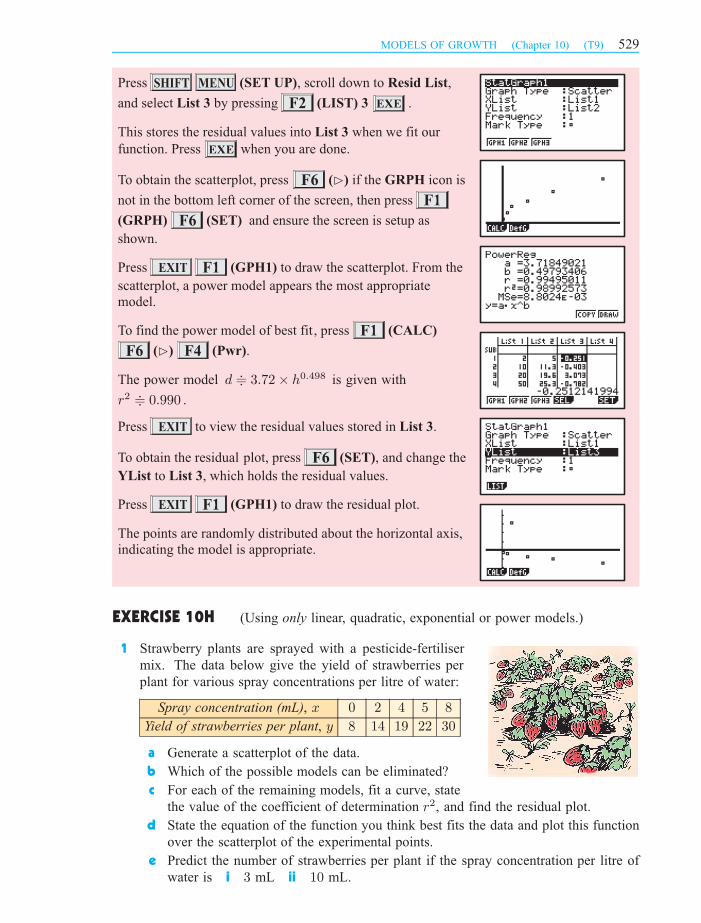
(Using only linear, quadratic, exponential or power models.)
1 Strawberry plants are sprayed with a pesticide-fertiliser
mix. The data below give the yield of strawberries per
plant for various spray concentrations per litre of water:
Spray concentration (mL), x 0 2 4 5 8
Yield of strawberries per plant, y 8 14 19 22 30
a Generate a scatterplot of the data.
b Which of the possible models can be eliminated?
c For each of the remaining models, fit a curve, state
the value of the coefficient of determination r2, and find the residual plot.
d State the equation of the function you think best fits the data and plot this function
over the scatterplot of the experimental points.
e Predict the number of strawberries per plant if the spray concentration per litre of
water is i 3 mL ii 10 mL.
EXERCISE 10H
Press (SET UP), scroll down to Resid List,
and select List 3 by pressing (LIST) 3 .
This stores the residual values into List 3 when we fit our
function. Press when you are done.
To obtain the scatterplot, press (¤) if the GRPH icon is
not in the bottom left corner of the screen, then press
(GRPH) (SET) and ensure the screen is setup as
shown.
Press (GPH1) to draw the scatterplot. From the
scatterplot, a power model appears the most appropriate
model.
To find the power model of best fit, press (CALC)
(¤) (Pwr).
Press to view the residual values stored in List 3.
To obtain the residual plot, press (SET), and change the
YList to List 3, which holds the residual values.
Press (GPH1) to draw the residual plot.
The points are randomly distributed about the horizontal axis,
indicating the model is appropriate.
The power model d + 3:72 £ h0:498 is given with
r2 + 0:990 .
MODELS OF GROWTH (Chapter 10) (T9) 529
F4
SA_11APPmagentacyan yellow black
0 05 5
25
25
75
75
50
50
95
95
100
100 0 05 5
25
25
75
75
50
50
95
95
100
100
Y:\HAESE\SA_11APP-2ed\SA11APP-2_10\529SA11APP-2_10.CDR Friday, 14 September 2007 10:46:22 AM DAVID3

2 Pinkie’s Pizza Parlour prices pepperoni pizzas as
follows:
Size (in inches), x 9 12 15 18
Cost ($), y 5:70 8:70 12:70 17:70
a Generate a scatterplot of the data.
b Can any of the possible models be eliminated?
c For each of the remaining models, fit a curve,
state the value of the coefficient of determina-
tion r2, and find the residual plot.
d State the equation of the function you think best
fits the data and plot this function over the scatterplot of the data points.
e If Pinkie plans to make 23 inch pizzas, predict the possible price.
3
Years since 1980, x 5 10 15 20 25
Population, y 730 995 1365 1870 2560
a Generate a scatterplot of the data.
b Which of the possible models can be eliminated?
c For the possible models remaining, fit a curve, state the value of the coefficient of
determination r2, and find the residual plot.
d State the equation of the ‘function of best fit’ and plot this function over the scat-
terplot of the data points.
e Predict the population of the villiage in: i 2015 ii 1965:
f Suggest reasons why your prediction in e ii may be inaccurate.
4 The maximum speed of a Chinese ‘dragonboat’ with increasing numbers of paddlers is
recorded in the table:
Number of paddlers, x 4 6 10 18 30
Maximum speed (kmph), y 8:7 10:2 12:6 15:9 19:5
a Draw a scatterplot of the data.
b Which of the possible models can be
eliminated?
c For the possible models remaining, fit
a curve, state the value of the coeffi-
cient of determination r2, and find the
residual plot.
d State the equation of the function that
you think best fits the data and plot
this function over the scatterplot of the experimental points.
e Predict the maximum speed of a dragonboat if there are:
i 24 paddlers ii 40 paddlers.
A remote village of hill tribes people was discovered in and its populationrecorded every years after . The results were:
19805 1980
530 MODELS OF GROWTH (Chapter 10) (T9)
SA_11APPmagentacyan yellow black
0 05 5
25
25
75
75
50
50
95
95
100
100 0 05 5
25
25
75
75
50
50
95
95
100
100
Y:\HAESE\SA_11APP-2ed\SA11APP-2_10\530SA11APP-2_10.CDR Thursday, 6 September 2007 12:31:21 PM PETERDELL
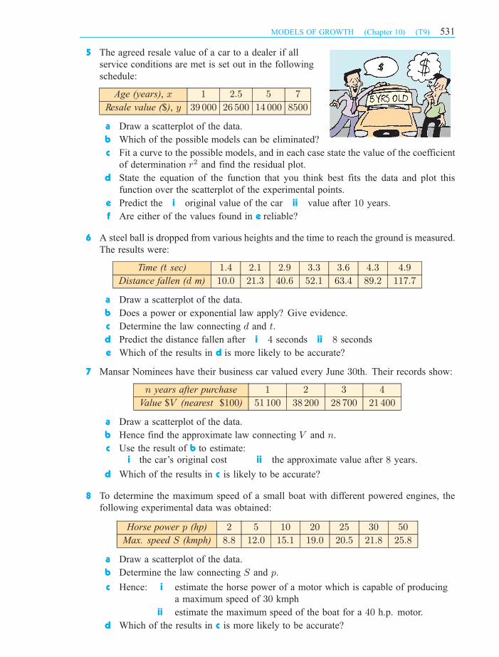
5 The agreed resale value of a car to a dealer if all
service conditions are met is set out in the following
schedule:
Age (years), x 1 2:5 5 7
Resale value ($), y 39 000 26 500 14 000 8500
a Draw a scatterplot of the data.
b Which of the possible models can be eliminated?
c Fit a curve to the possible models, and in each case state the value of the coefficient
of determination r2 and find the residual plot.
d State the equation of the function that you think best fits the data and plot this
function over the scatterplot of the experimental points.
e Predict the i original value of the car ii value after 10 years.
f Are either of the values found in e reliable?
6 A steel ball is dropped from various heights and the time to reach the ground is measured.
The results were:
Time (t sec) 1:4 2:1 2:9 3:3 3:6 4:3 4:9
Distance fallen (d m) 10:0 21:3 40:6 52:1 63:4 89:2 117:7
a Draw a scatterplot of the data.
b Does a power or exponential law apply? Give evidence.
c Determine the law connecting d and t.
d Predict the distance fallen after i 4 seconds ii 8 seconds
e Which of the results in d is more likely to be accurate?
7 Mansar Nominees have their business car valued every June 30th. Their records show:
n years after purchase 1 2 3 4
Value $V (nearest $100) 51 100 38 200 28 700 21 400
a Draw a scatterplot of the data.
b Hence find the approximate law connecting V and n.
c Use the result of b to estimate:i the car’s original cost ii the approximate value after 8 years.
d Which of the results in c is likely to be accurate?
8 To determine the maximum speed of a small boat with different powered engines, the
following experimental data was obtained:
Horse power p (hp) 2 5 10 20 25 30 50
Max. speed S (kmph) 8:8 12:0 15:1 19:0 20:5 21:8 25:8
a Draw a scatterplot of the data.
b Determine the law connecting S and p.
c Hence: i estimate the horse power of a motor which is capable of producing
a maximum speed of 30 kmph
ii estimate the maximum speed of the boat for a 40 h.p. motor.
d Which of the results in c is more likely to be accurate?
MODELS OF GROWTH (Chapter 10) (T9) 531
SA_11APPmagentacyan yellow black
0 05 5
25
25
75
75
50
50
95
95
100
100 0 05 5
25
25
75
75
50
50
95
95
100
100
Y:\HAESE\SA_11APP-2ed\SA11APP-2_10\531SA11APP-2_10.CDR Thursday, 6 September 2007 12:31:27 PM PETERDELL

PROJECT THE PENDULUM
9 The table below shows the concentration of chemical X in the blood at various times
after an injection was administered.
Time (t minutes) 10 20 30 40 50 60 70
Concentration of X
(C micrograms/cm3)104:6 36:5 12:7 4:43 1:55 0:539 0:188
a Draw a scatterplot of the data.
b Hence determine the approximate exponential law connecting C and t.
c If the injection is effective while the concentration of X is greater than
2 £ 10¡4 micrograms/cm3, how long will it take before the injection ‘wears off’?
10 The table below shows the temperature of a cup of coffee as it cools. Note that the
temperature T oC is the temperature above room temperature.
Time of cooling (t minutes) 5 10 15 20 25 30 35
Temperature (T oC aboveroom temperature)
31:5 13:3 5:6 2:3 1:0 0:41 0:17
a Draw a scatterplot of the data.
b
c If room temperature was constant at 20oC throughout the cooling, estimate the
temperature of the coffee when the experiment started.
d Estimate the temperature of the coffee after it has been cooling for 2 minutes.
1 Which of the following ideas have merit when finding the period of the pendulum for
a particular length?
² Several students should time one period using their stopwatches.
² Timing 8 complete swings and averaging is better than timing one complete swing.
² If several students do the timing, the highest and lowest scores should be removed
and the remaining scores should be averaged.
2 List possible factors which could lead to inaccurate results.
A can be made by tying an object such as a mobile phone to ashoe lace and allowing the object to swing back and forth when supportedby the string.
pendulum
We will find the , which is the time taken forone complete oscillation, back and forth, for variouslengths of the pendulum.
The maximum angle of the pendulum should be .The length of the pendulum is the distance from thepoint of support to the object’s centre of mass.
period
µ 15o
What to do:
The object of this investigation is to determine any rule which mayconnect the period of the pendulum ( secs) with its length ( cm).T l
l cm
point ofsupport
��
object
Determine the law connecting T and t.
532 MODELS OF GROWTH (Chapter 10) (T9)
SA_11APPmagentacyan yellow black
0 05 5
25
25
75
75
50
50
95
95
100
100 0 05 5
25
25
75
75
50
50
95
95
100
100
Y:\HAESE\SA_11APP-2ed\SA11APP-2_10\532SA11APP-2_10.CDR Friday, 14 September 2007 9:43:44 AM DAVID3

REVIEW SET 10
3 After deciding on a method for determining the
period, measure the period for pendulum lengths
of 20 cm, 30 cm, 40 cm, ...., 100 cm and record
your results in a table like the one alongside.
length (l cm) period (T s)
203040...4 Use technology to determine the law connecting
T and l.
1 A population of seals t years after a colony was noticed is given by Pt = 40£ 20:3t,t > 0. Find:
a the initial size of the population
b the population after
i 5 years ii 10 years iii 20 years.
c Sketch the graph of Pt against t using only your results from a and b.
d Use technology to graph Y1 = 40£ 20:3t and check your answers to a, b and c.
2 The weight of a radioactive substance after t years is given by the formula
Wt = 5 £ 3¡0:003t grams. Find:
a the initial weight of the radioactive substance
b the percentage remaining after
i 100 years ii 500 years iii 1000 years.
c Graph Wt against t.
3 a What is the total energy released by an earthquake of magnitude 7:2 on the
Richter scale?
b What increase in ground movement occurs between two earthquakes with mag-
nitudes 3:4 and 5:1?
4 How many times louder is a sound of 82 decibels than a sound of 42 decibels?
5 The figures below show the number of surviving beetles in a square metre of lawn
two days after it was sprayed with a new chemical.
Amount of chemical (x grams) 2 3 5 6 9
Number of lawn beetles (y) 11 8 6 4 3
a Draw a scatterplot for this data.
b Determine the r and r2 values for the linear model.
c Describe the association between the number of lawn beetles and the amount of
chemical sprayed.
d Use your technology to determine the equation of the line of best fit.
e Give an interpretation for the slope and vertical intercept of this line.
f Use your equation to predict the amount of chemical required to remove all lawn
beetles.
MODELS OF GROWTH (Chapter 10) (T9) 533
SA_11APPmagentacyan yellow black
0 05 5
25
25
75
75
50
50
95
95
100
100 0 05 5
25
25
75
75
50
50
95
95
100
100
Y:\HAESE\SA_11APP-2ed\SA11APP-2_10\533SA11APP-2_10.CDR Thursday, 6 September 2007 12:31:37 PM PETERDELL

The following table shows the profit figures for McKenzie Mattresses over a yearperiod:
76
a Use technology to draw a scatterplot for this data.
b Determine the r and r2 values for the linear model.
c Find the equation of the line of best fit and comment on its reliability to predict
future profits.
7 Write as a power of 3:
a 81 b 1 c 1
27d 1
243
8 Write as a power of 2:
a 1
4b 32 c
1p2
dp
8
9 Write as a single power of 2 or 3: a 4a £ 8 b4x+2
21¡xc
27
9a
10 Write without negative indices:
a mn¡2 b (mn)¡3 c³mn
´¡2
d (4m¡1n)2
11 Without using a calculator, write in simplest rational form:
a 843 b 27
43 c 32¡
25 d 25¡
32
12 On the same set of axes draw the graphs of:
a y = 2x and y = 2x + 2 b y = 2x and y = 2x+2
13 Sketch the graph of y = 2¡x ¡ 5:
14 Sketch the graph of y = 4 ¡ 2x.
15 Without using a calculator, solve for x: a 27x = 3 b 91¡x = 1
3
16 Solve for x, giving your answer correct to 3 significant figures:
a 5x = 7 b 20 £ 20:5x = 500 c 53¡x = 32x+1
17 The weight W grams, of radioactive substance remaining after t years is given by
W = 500 £ 2¡0:05t grams. Find the time taken for the weight to:
a halve b reach 50 grams
18
a Draw a scatterplot of the data
b Hence determine the law connecting P and t.
c Estimate the population number after i 18 months ii 8 years
d Which of the results in c is reliable?
The table below shows the population numbers of a colony of albatross years afterthe colony was established.
t
Year 2000 2001 2002 2003 2004 2005 2006
profit ($ £ 1000) 17 24 20 27 23 38 31
Time (t years) 0 1 2 3 4
Population (P ) 208 282 383 521 707
534 MODELS OF GROWTH (Chapter 10) (T9)
SA_11APPmagentacyan yellow black
0 05 5
25
25
75
75
50
50
95
95
100
100 0 05 5
25
25
75
75
50
50
95
95
100
100
Y:\HAESE\SA_11APP-2ed\SA11APP-2_10\534SA11APP-2_10.CDR Thursday, 6 September 2007 12:31:42 PM PETERDELL

19
Distance (d m) 10 20 30 40
Time (t sec) 1:43 2:02 2:47 2:86
a Generate a scatterplot of the data.
b Which of the possible function models can be eliminated?
c For each of the remaining models, fit a curve, calculate the value of the coefficient
of determination r2, and find the residual plot.
d State the equation of the ‘function of best fit’ and plot this function over the
scatterplot of experimental points.
e Predict the time taken for the stone to fall 25 m.
20 The concentration of chemical Y in the blood of an accident victim at various times
after an injection was administered is recorded in the table below:
a Generate a scatterplot of the data.
b Which of the possible function models can be
eliminated?
c For the possible function models, fit a curve,
calculate the value of the coefficient of deter-
mination r2, and find the residual plot.
d State the equation of the ‘function of best fit’
and plot this function over the scatterplot of
the experimental points.
e Predict the concentration of chemical Y after 40 minutes.
21 The value of a rare stamp t years after it was purchased is given by
V (t) = 100 £ 20:2t dollars.
a Sketch the graph of V (t) for t > 0.
b Find the value of the stamp (to the nearest dollar) 7 years after it was purchased.
c When will the value of the stamp reach $1000?
22 Alex sells cartons of milk in his store. In the past, he has altered the price of his
milk, and the table below shows the weekly profit received when the milk was sold
at various prices:
a Draw a scatterplot for this data.
b Which of the possible function models is the best fit for the data? Explain.
c Find the equation of the ‘function of best fit’, and state the value of r2.
d Predict Alex’s weekly profit if he sells his milk for: i $1:85 ii $2:35.
The time taken ( secs) for a stone to fall various distances ( m) was observed andrecorded in the given table.
t d
Price ($p) 1:75 2:10 1:90 1:60 2:25 2:00
Profit ($P / week) 129 135 140 105 113 138
Time (t minutes) 5 10 15 20 25 30 35
Concentration of Y
(C micrograms/cm3)29 18 12 7:3 4:7 2:9 1:8
MODELS OF GROWTH (Chapter 10) (T9) 535
SA_11APPmagentacyan yellow black
0 05 5
25
25
75
75
50
50
95
95
100
100 0 05 5
25
25
75
75
50
50
95
95
100
100
Y:\HAESE\SA_11APP-2ed\SA11APP-2_10\535SA11APP-2_10.CDR Thursday, 6 September 2007 12:31:48 PM PETERDELL

e Which of the predictions in d is likely to be more accurate?
f What price should Alex set for his milk to maximise his profit?
23 The pulse rate of a runner t minutes after he finishes
training is given by P (t) = 90£ 3¡0:25t + 50 beats
per minute.
a Sketch the graph of P (t) for t > 0.
b Find the runner’s pulse rate immediately after he
finished training.
c How long did it take for his pulse rate to drop to:
i 70 beats per minute ii 55 beats per minute?
24 The table below shows the amount of television watched per week by a group of
students, as well as their score (out of 100) in a recent examination.
a Draw a scatterplot for this data.
b Explain why a linear model appears most appropriate.
c Find the least squares ‘line of best fit’ for the data, and state the values of r and
r2.
d Describe the association between examination score and television watched.
e Predict the examination score for a student who watches television for
i 14 hours per week ii 25 hours per week?
25 Seven students, who live varying distances from their school, were asked how long it
takes them to get to school each morning. The results were:
a Draw a scatterplot for this data.
b Kevin thinks the data looks linear, but Caitlin thinks it looks like a power model.
Find the ‘function of best fit’, state the value of r2 and draw a residual plot for:
i a linear model ii a power model.
c Which model appears to fit the data better? Explain.
d Kevin lives 15 km from school. Using the model chosen in c, predict how long
it takes Kevin to get to school each morning.
Television watched (t hours/week) 5 20 8 2 16
Examination score (S) 87 62 81 91 70
Distance from school (d km) 13 2 17 8 28 3 10
Time (T min) 23 6 28 16 40 8 19
536 MODELS OF GROWTH (Chapter 10) (T9)
SA_11APPmagentacyan yellow black
0 05 5
25
25
75
75
50
50
95
95
100
100 0 05 5
25
25
75
75
50
50
95
95
100
100
Y:\HAESE\SA_11APP-2ed\SA11APP-2_10\536SA11APP-2_10.CDR Thursday, 6 September 2007 12:31:53 PM PETERDELL