1

Week 9MPLS: Multiprotocol Label

Switching

3

MPLS…What is it?

MPLS – Multi-protocol Label Switching can be applied for any layer 2 network

protocol

MPLS is a natural evolution of Internet It is based on IP and routing protocols such

as BGP-4,OSPF and IS-IS

Typically MPLS resides in service providers networks and not in private networks

4

MPLS Protocol Stack

Physical

Layer 2 (PPP, ATM, FR,..)

MPLS

IP or Multi-Service

Application

5

What is MPLS ?

MPLS provides connection oriented switching based on a label applied at the edge of an MPLS domain.

IP is used to signal MPLS connections. Major Applications are:

Network Scalability Traffic Engineering VPNs

6

MPLS - Best Of Both WorldsPACKETForwarding

PacketSWITCHING

MPLSIP ATM/FR

HYBRID

1. Scalable2. Flexible3. Easily Deployable4. Inexpensive5. Dynamic Routing

1. Performance2. Connection Oriented3. Traffic Engineering4. Security5. QoS

Route at the Edge & Switch at the Core

7

Why MPLS ?

MPLS converts connectionless IP to a connection- oriented mode

MPLS allows IP to be switched through the Internet instead of routed

With MPLS the first IP packet of a stream establishes a switched path for all subsequent packets to follow

The packets will only be switched at each hop and not routed.

8

Towards a connection-oriented IP.. MPLS is the evolution of current IP and

connection oriented protocols Strength and scalability of IP routing

PVC like connectivity

ATM like QoS

Explicit routing

Plus Path protection

Path optimization

9

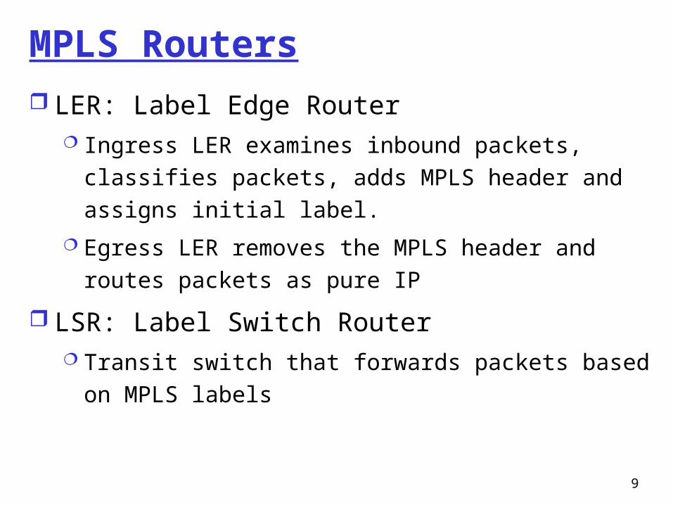
MPLS Routers LER: Label Edge Router

Ingress LER examines inbound packets, classifies packets, adds MPLS header and assigns initial label.

Egress LER removes the MPLS header and routes packets as pure IP

LSR: Label Switch Router Transit switch that forwards packets based on

MPLS labels

10

IP and MPLS Forwarding

IP packets are classified into FECs (Forwarding Equivalence Class) at each hop based on the destination address in conventional routing

IP packet forwarding works by assigning a packet to a FEC

determining the next-hop of each FEC

MPLS group Packets by assigning a label in to FEC

based on Class of Service (CoS) and forward fast in a defined path with the same forwarding treatment

11

Traditional IP Forwarding

47.1

47.247.3

IP 47.1.1.1

Dest Out

47.1 147.2 2

47.3 3

1

23

Dest Out

47.1 147.2 2

47.3 3

1

2

1

2

3

IP 47.1.1.1

IP 47.1.1.1IP 47.1.1.1

Dest Out

47.1 147.2 2

47.3 3

12

Label Switch Path (LSP) LSP: Label Switched Path

– Simplex L2 tunnel

– Equivalent of Virtual Circuit

4 Byte Label is inserted in to the IP Packet at egress MPLS node to Switch IP alone the created Label Switch Path (LSP)

Such MPLS nodes are called Label Switch Routers (LSR).

With Labels IP Packet header is analyzed only at ingress and egress LSRs where Labels are inserted and removed.

Labels only have a Local significance and change from hop to hop on the MPLS network. (Like DLCI in FR and VCI/VPI in ATM)

13

Label Swapping

Label Push: When an IP Packet enters the MPLS network the Label is inserted by ingress LSR

Label Pop: When the IP Packet exits the MPLS network the Label is removed by the egress LSR

The Label is swapped at each intermediate hop based on a Label mapping table

Label mapping table is called the Label Information Base (LIB)

14

MPLS Header

Label: Label value, 20 bits Exp: Experimental (CoS), 3 bits

ToS /DSCP to Exp mapping

S: Bottom of stack, 1 bit

TTL: Time to Live, 8 bit

– Ingress LER sets MPLS TTL to IP TTL

– Egress LER may set IP TTL to MPLS TTL or not

15

MPLS Operation

Egress LSR removes label beforeforwarding IP packets

outside MPLSnetwork

Standard Routing protocols

Labels are exchanged .

LSR LSRLSRLSR

IP ForwardingLABEL SWITCHINGIP Forwarding

LSRs forwardpackets based on

the label (no packet classification

in the core)

Ingress LSR receives IP packets, performs packet classification

(into FECs), assigns a label, &forwards the labeled packet

Label

IP Hdr

Payload +

Ingress Egress

16

MPLS Packet Flow

Step 1: Ingress LER classifies IP packet , adds MPLS header and assigns label

Step 2: Transit LSR forwards label packet using label swapping

Step 3: Egress LER removes MPLS header and performs IP processing

17

MPLS IP forwarding via LSP

IntfIn

LabelIn

Dest IntfOut

3 0.40 47.1 1

IntfIn

LabelIn

Dest IntfOut

LabelOut

3 0.50 47.1 1 0.40

47.1

47.247.3

1

2

31

2

1

2

3

3

IntfIn

Dest IntfOut

LabelOut

3 47.1 1 0.50

IP 47.1.1.1

IP 47.1.1.1

18

MPLS Terminology

LDP: Label Distribution Protocol

LSP: Label Switched Path

FEC: Forwarding Equivalence Class

LSR: Label Switching Router

LER: Label Edge Router (Useful term not in

standards)

19

Forwarding Equivalence Classes

• FEC = “A subset of packets that are all treated the same way by a router”

• The concept of FECs provides for a great deal of flexibility and scalability

• In conventional routing, a packet is assigned to a FEC at each hop (i.e. L3 look-up), in MPLS it is only done once at the network ingress

Packets are destined for different address prefixes, but can bemapped to common pathPackets are destined for different address prefixes, but can bemapped to common path

IP1

IP2

IP1

IP2

LSRLSRLER LER

LSP

IP1 #L1

IP2 #L1

IP1 #L2

IP2 #L2

IP1 #L3

IP2 #L3

20

#216

#612

#5#311

#14

#99

#963

#462

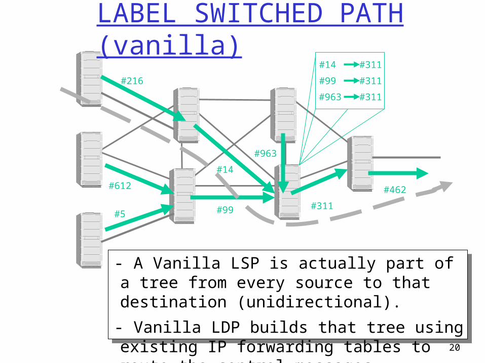
- A Vanilla LSP is actually part of a tree from every source to that destination (unidirectional).

- Vanilla LDP builds that tree using existing IP forwarding tables to route the control messages.

#963

#14

#99

#311

#311

#311

LABEL SWITCHED PATH (vanilla)

21

MPLS BUILT ON STANDARD IP

47.1

47.247.3

Dest Out

47.1 147.2 2

47.3 3

1

23

Dest Out

47.1 147.2 2

47.3 3

Dest Out

47.1 147.2 2

47.3 3

1

23

1

2

3

• Destination based forwarding tables as built by OSPF, IS-IS, RIP, etc.

22

IP FORWARDING USED BY HOP-BY-HOP CONTROL

47.1

47.247.3

IP 47.1.1.1

Dest Out

47.1 147.2 2

47.3 3

1

23

Dest Out

47.1 147.2 2

47.3 3

1

2

1

2

3

IP 47.1.1.1

IP 47.1.1.1IP 47.1.1.1

Dest Out

47.1 147.2 2

47.3 3

23

IntfIn

LabelIn

Dest IntfOut

3 0.40 47.1 1

IntfIn

LabelIn

Dest IntfOut

LabelOut

3 0.50 47.1 1 0.40

MPLS Label Distribution

47.1

47.247.3

1

2

31

2

1

2

3

3IntfIn

Dest IntfOut

LabelOut

3 47.1 1 0.50 Mapping: 0.40

Request: 47.1

Mapping: 0.50

Request: 47.1

24

Label Switched Path (LSP)

IntfIn

LabelIn

Dest IntfOut

3 0.40 47.1 1

IntfIn

LabelIn

Dest IntfOut

LabelOut

3 0.50 47.1 1 0.40

47.1

47.247.3

1

2

31

2

1

2

3

3IntfIn

Dest IntfOut

LabelOut

3 47.1 1 0.50

IP 47.1.1.1

IP 47.1.1.1

25

Label Distribution Protocols The network automatically builds the routing tables

by IGP protocols such as OSPF, IS-IS. The label distribution protocol (LDP) uses the established routing topology to route the LSP request path between adjacent LSRs.

A LDP is a set of procedures by which one LSR informs another LSR of the label to FEC bindings it has made.

The LDP also encompasses any negotiations in which two label distribution peers (Ingress LSR and egress LSR) need to engage in order to offer CoS to particular IP stream.

26

Hop-by-hop routed LSPA

C D

BE0 1

2

2

10

0

12

0

21

0

Incoming Label

Outgoing Label

Next hop Outgoing Interface

A 100 ? B 1

B 6 ? E 1

C 17 ? D 2

D 5 ? E 0

E 6 ? E 0

192.6/16

27

Example Contd

Incoming Label

Outgoing Label

Next hop Outgoing Interface

A 100 6 B 1

B 6 6 E 1

C 17 5 D 2

D 5 6 E 0

E 6 ? E 0

28

#216

#14

#462

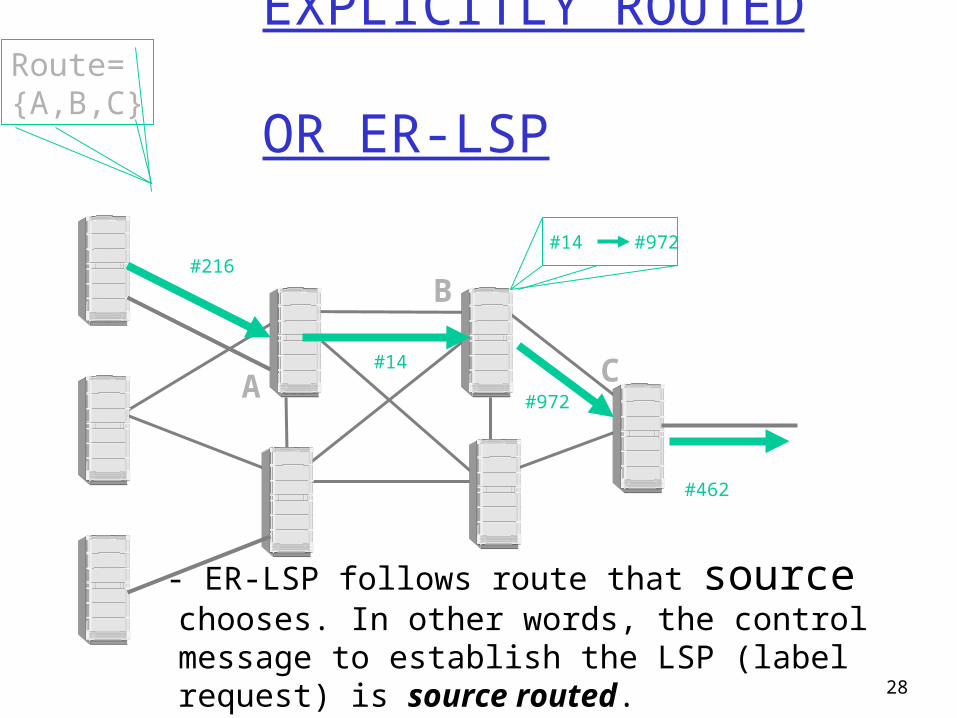
- ER-LSP follows route that source chooses. In other words, the control message to establish the LSP (label request) is source routed.

#972

#14 #972

A

B

C

Route={A,B,C}

EXPLICITLY ROUTED OR ER-LSP

29

IntfIn

LabelIn

Dest IntfOut

3 0.40 47.1 1

IntfIn

LabelIn

Dest IntfOut

LabelOut

3 0.50 47.1 1 0.40

47.1

47.247.3

1

2

31

2

1

2

3

3

IntfIn

Dest IntfOut

LabelOut

3 47.1.1 2 1.333 47.1 1 0.50

IP 47.1.1.1

IP 47.1.1.1

EXPLICITLY ROUTED LSP ER-LSP

30

ER LSP - advantages

•Operator has routing flexibility (policy-based, QoS-based)

•Can use routes other than shortest path

•Can compute routes based on constraints in exactly the same manner as ATM based on distributed topology database.(traffic engineering)

31

Routing Scalability via MPLS

Routing Domain A

Routing Domain B

Routing Domain C

V

T

X

Y

W Z

32

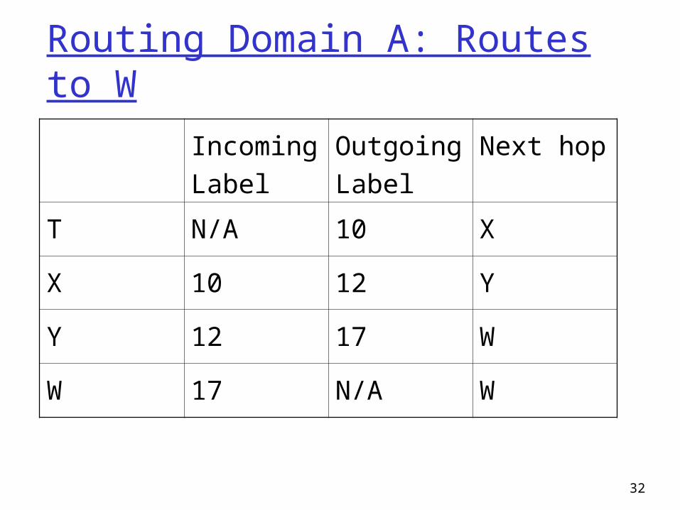
Routing Domain A: Routes to W

Incoming Label

Outgoing Label

Next hop

T N/A 10 X

X 10 12 Y

Y 12 17 W

W 17 N/A W

33

Example Contd – Label Stacking

Routing Domain A

Routing Domain B

Routing Domain C

V

T

X

Y

W Z5

102

122

172

6

34

Routing Transients

Routing transients happen due to failure detection (in the order of milliseconds)

LSP dissemination (in the order of propagation delays)

SPF tree calculation (in the order of several hundred milliseconds)

R1

R2

R3

R4

R5

35

MPLS Example

Setup: PATH (ERO = LSR1, LSR2, LSR4, LSR9)

LSR1

LSR8

LSR2

LSR6 LSR7

LSR4

LSR9

LSR5

Labels established on RESV message

Pop

14

37

36

Fast Reroute - Protection Path

Setup: PATH (LSR2, LSR6, LSR7, LSR4)

LSR1

LSR8

LSR2

LSR6 LSR7

LSR4

LSR9

LSR5

Labels established on RESV message

17

22

Pop

37

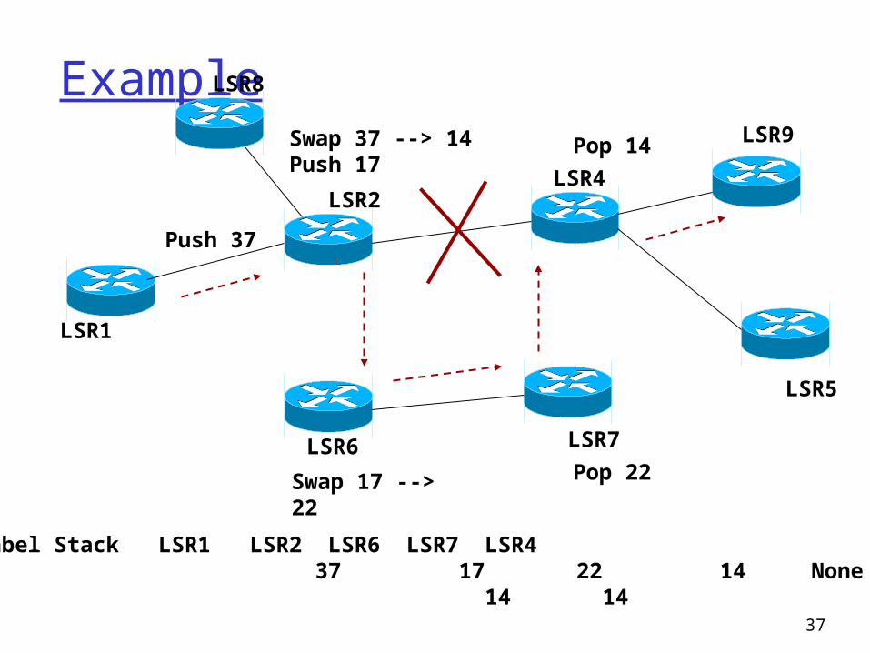
Example

LSR1

LSR8

LSR2

LSR6 LSR7

LSR4

LSR9

LSR5

Push 37

Swap 37 --> 14Push 17

Swap 17 --> 22 Pop 22

Pop 14

Label Stack LSR1 LSR2 LSR6 LSR7 LSR4 37 17 22 14 None 14 14

38

MPLS Protection May result in suboptimal forwarding but service

interruption is negligible

A single protection LSP could be used to fast-route not one but multiple LSPs

Protection on a per-LSP basis (end-to-end) rather than on a per-link basis is also possible better forwarding properties in case of failures

a single protection may not protect as many LSPs

handles both node and link failures

detection time may be larger

will require the computation of link and node disjoint paths

39

Label Encapsulation

ATM FR Ethernet

PPP

MPLS Encapsulation is specified over various media types. Top labels may use existing format, lower label(s) use a new “shim” label format.

VPI VCI DLCI “Shim Label”

L2

Label

“Shim Label” …….

IP | PAYLOAD

40

Traffic Engineering - Objectives

Performance optimization of operational networks. Reduce congestion hot spots. Improve resource utilization.

Why current IP routing is not sufficient from TE perspective? Fish problem. Destination-based Local optimization

R8

R2

R6

R3

R4

R7

R5

R1

IP Routing & “the Fish”

IP (Mostly) Uses Destination-Based Least-Cost RoutingFlows from R8 and R1 Merge at R2 and Become IndistinguishableFrom R2, Traffic to R3, R4, R5 Use Upper Route

Alternate Path Under-Utilized

6

42

Deficiencies in IP Routing

Chronic local congestion

Load balancing Across long haul links

Size of links Difficult to get IP to make good use unequal

size links without overloading the lower speed link

43

Peer Model

Peer model OSPF routing + link weights.

Key technique: weight setting.

Networks operate as it does today.

Much more scalable than overlay model.

44

Load Balancing

Making good use of expensive links simply by adjusting IGP metrics can be a frustrating exercise!

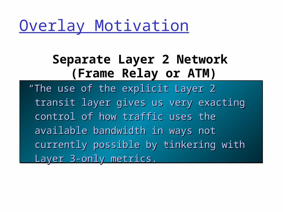
Overlay Motivation

Separate Layer 2 Network (Frame Relay or ATM)

““The use of the explicit Layer 2 transit The use of the explicit Layer 2 transit

layer gives us very exacting control of layer gives us very exacting control of

how traffic uses the available how traffic uses the available

bandwidth in ways not currently bandwidth in ways not currently

possible by tinkering with Layer 3-only possible by tinkering with Layer 3-only

metrics.”metrics.”

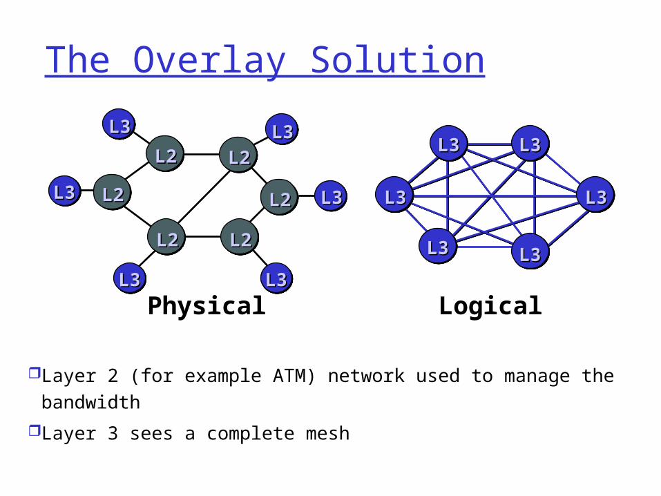
The Overlay Solution

Layer 2 (for example ATM) network used to manage the bandwidth

Layer 3 sees a complete mesh

L3L3

L3L3

L3L3

L3L3

L3L3

L3L3

L3L3

L2L2

L2L2

L2L2

L2L2

L2L2

L2L2

L3L3

L3L3

L3L3

L3L3 L3L3

Physical Logical

Overlay Drawbacks

Extra network devices (cost)

More complex network managementTwo-level network without integrated NM

Additional training, technical support, field engineering

IGP routing doesn’t scale for meshesNumber of LSPs generated for a failed router is O(n3); n = number of routers

48

Overlay Drawbacks Every router is permanently connected to every other

router (fullmesh) PVCs are provisioned with given bandwidths Delays are short Problem: scalability

• For N routers, N x (N-1)/2 ATM VCs• Also:• The IP link-state routing protocol (e.g. OSPF) has to handle a huge

number of links, and link State Advertisements packets are flooded on every link

Worse: when an ATM link fails, all VCs using that link fail, andmany IP routers have to update their routing tables at the same time

Amount of routing information can be as much as N^4 In practice, this solution does not scale beyond 100

routers (± 5000 PVCs)

Traffic Engineering & MPLS

MPLS fuses Layer 2 and Layer 3Layer 2 capabilities of MPLS can

be exploited for IP traffic engineering

Single box / network solution

+ oror=

Router ATM Switch MPLS Router

ATM MPLS Router

50

An LSP Tunnel

R8

R2

R6

R3

R4

R7

R5

R1

Normal Route R1->R2->R3->R4->R5

Tunnel: R1->R2->R6->R7->R4

Labels, like VCIs can be used to establish virtual circuits

51

Comprehensive Traffic Engineering Network design

Engineer the topology to fit the traffic

Traffic engineering Engineer the traffic to fit the topology

Given a fixedfixed topology and a traffic matrix, traffic matrix, what set of explicit routes offers the best overall network performance?

52

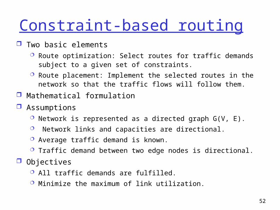
Constraint-based routing Two basic elements

Route optimization: Select routes for traffic demands subject to a given set of constraints.

Route placement: Implement the selected routes in the network so that the traffic flows will follow them.

Mathematical formulation Assumptions

Network is represented as a directed graph G(V, E). Network links and capacities are directional. Average traffic demand is known. Traffic demand between two edge nodes is directional.

Objectives All traffic demands are fulfilled. Minimize the maximum of link utilization.

53

Off-line Formulation

Notations G=(V,E) cij be the capacity of link (i,j), for all (i,j) in E. K: the set of traffic demands between a pair of

edge nodes. (dk,sk,tk): (bandwidth demand, source node,

destination node), for all k in K. Xij

k the percentage of k’s bandwidth demand satisfied by link (i,j).

α: the maximum of link utilization among all the links.

54

Off-line Formulation

55

On-line TE

Shortest path (SP) Link metric for link (i,j) is inversely

proportional to the bandwidth.

Minimize the total resource consumption per route. Minimum hop (MH)

Link metric is set to 1 uniformly for each hop.

Still run shortest path algorithm.

56

On-line TE

Shortest-widest path (SWP) Link metric is set to as bandwidth. Always selecting the path with largest bottleneck

bandwidth. The one with minimum hops or shortest distance is

chosen when multiple paths are available.

Hybrid algorithm Motivation. Solution: appropriate weight assignment, and link

utilization (instead of using link residual bandwidth). Metric: path cost + link utilization.

57

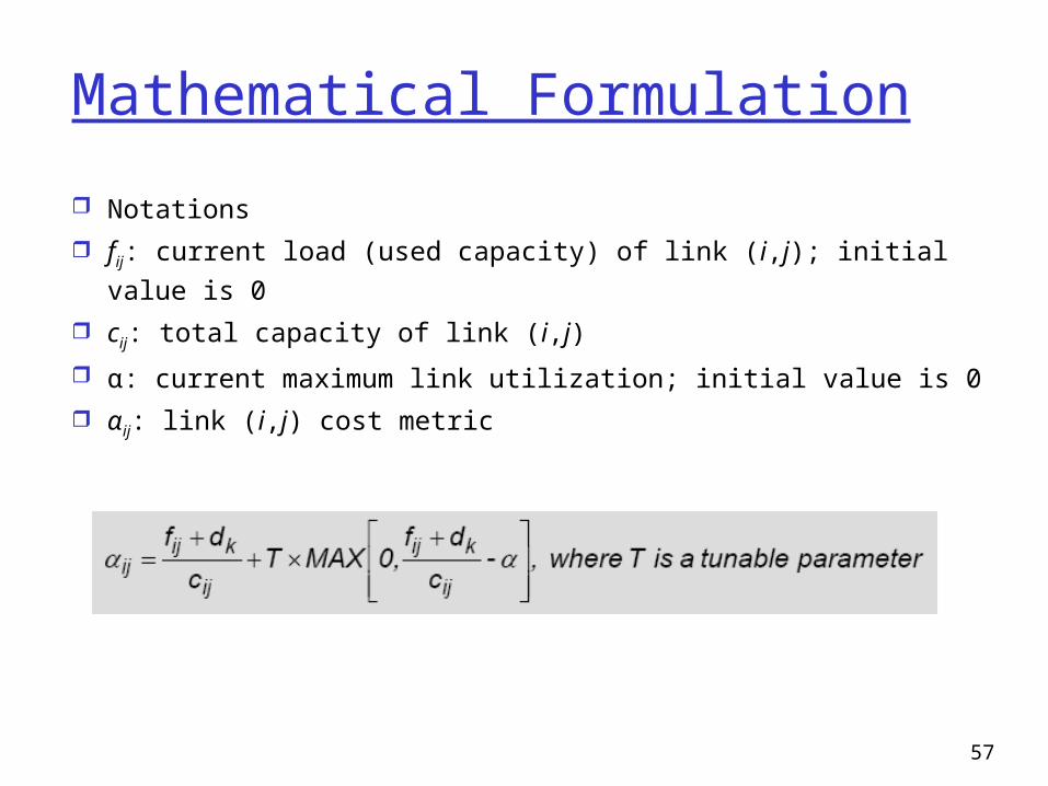
Mathematical Formulation

Notations

fij: current load (used capacity) of link (i,j); initial value is 0

cij: total capacity of link (i,j)

α: current maximum link utilization; initial value is 0

αij: link (i,j) cost metric

58

Multi-path Algorithms

TrafficSplitter

Incoming Traffic

Outgoing Traffic

L1

L2

59

Traffic Splitting

Basic requirements Traffic splitting is in the packet-forwarding path, and

executed for every packet.

To reduce implementation complexity, the system should preferably keep no or little state info.

Traffic-splitting schemes produce stable traffic distribution across multiple outgoing links with minimum fluctuation.

Traffic-splitting algorithms must maintain per-flow packet ordering.

60

Hashing

Direct hashing Hashing of destination address H(•)=DestIP mod N N: the number of outgoing links

Hashing using XOR folding of source/destination addresses

H(•)=(S1⊗S2⊗S3⊗S4⊗D1⊗D2⊗D3⊗D4) mod N ⊗: XOR operation Si: the ith octet of the source address Di: the ith octet of the destination address CRC 16 (16-bit cyclic redundant checksum)

H(•)=CRC16(5-tuple) mod N (−) distributing traffic load evenly

61

Hashing

Split a traffic stream into M bins.

The M bins are mapped to N outgoing links based on an allocation table, i.e., compute the corresponding hash value.

By changing the allocation of the bins to the outgoing links, we can distribute traffic in a predefined ratio.

1 N

2 1

3 1

4 N

M-1 3

M 1

1

N

62

• Introduction

• Traffic Engineering (TE)

• Problem Statement

• Our Proposed TE Architecture

• Path Establishment

• Queuing Models

• Feedback Mechanism and Rate Control

• Traffic Splitting Algorithm

• Simulations

• Conclusion

Bilkent’s Traffic Engineering

Onur Alparslan’s MS thesis work

63

Definition: The process of controlling how traffic flows through a network so as to optimize resource utilization and network performance, and reconfiguration of mapping in changing network conditions.

Advantages: • Provide ISPs precise control over the placement of traffic

flows.

• Balance the traffic load on the various links, routers, and switches in the network so that none of these components is overutilized or underutilized.

• Provide more efficient use of available aggregate bandwidth.

• Avoid hot spots in the network.

Traffic Engineering (TE)

64

Our Goal:

• Our main aim is to increase total amount of carried traffic and balance the load of links in the network by using two disjoint paths (multipath).

• No need for prior information on traffic matrix.

• Eliminate knock-on effect.

• Consider the load balancing performance of elastic TCP flows.

• Apply methods that are TCP friendly

• Capabilities to simulate a mesh network with thousands of TCP flows by using ns-2

Problem Statement

65

Our Approach:

• A primary and a disjoint secondary path are established from an ingress node to each egress node.

• Split TCP traffic between the primary and secondary paths using a distributed mechanism based on ECN marking and AIMD-based rate control.

• Primary paths have strict priority over the secondary paths with respect to packet forwarding

• TCP splitting mechanism operates on a per-flow basis in order to prevent packet reordering which can substantially reduce TCP performance

Problem Statement

66

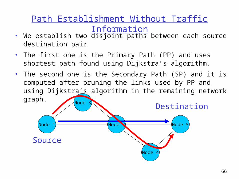
Path Establishment Without Traffic Information

• We establish two disjoint paths between each source destination pair

• The first one is the Primary Path (PP) and uses shortest path found using Dijkstra’s algorithm.

• The second one is the Secondary Path (SP) and it is computed after pruning the links used by PP and using Dijkstra’s algorithm in the remaining network graph.

Node 3

Node 2Node 1 Node 5

Node 4

Source

Destination

67

Queuing ModelBackbone Network

Per-egress queuing Per-class queuing

Egress Node 2

Egress Node 1

PP Queue

SP Queue

Silver Queue

Bronze Queue

Gold Queue

RM + TCP ACK

SP Queue

PP Queue

Egress Node 0

68

• Giving equal priority to PPs and SPs may decrease the performance of PPs since a SP may share links with PPs of other node pairs

• Traffic increase on a SP may force sources of PPs sharing links with this SP to move traffic to their own SPs

• This further decreases performance, because SPs typically use longer routes and can also force other PPs to move traffic to their SPs

Knock-on Effect

Edge 3

Edge 2Edge 1

69

Bistability in Single Overlay: Phone Network Phone network is an overlay

Logical link between each pair of switches

Phone call put on one-hop path, when possible

… and two-hop alternate path otherwise

Problem: inefficient path assignment Two-hop path for one phone call

… stops another call from using direct path

… forcing the use of a two-hop alternate path

busy

busy

70

Preventing Inefficient Routes: Trunk Reservation

Two stable states for the system Mostly one-hop calls with low blocking rate

Mostly two-hop calls with high blocking rate

Making the system stable Reserve a portion of each link for direct calls

When link load exceeds threshold…

• … disallow two-hop paths from using the link

Rejects some two-hop calls

• … to keep some spare capacity for future one-hop calls

Stability through trunk reservation Single efficient, stable state with right threshold

71

FIFO (First In First Out) Queuing• TCP data packets of PPs and SPs join the same silver queue and

we do not make use of the Bronze Queue at all

• ACK and Probe Packets (RM) join the Gold Queue

• Gold Queue has strict priority over Silver Queue.

Gold Silver

Core Router

ACK

Probe Packet (RM)

PP Data Packet

SP Data Packet

72

SP (Strict Priority) Queuing• Data packets of PPs enter Silver Queue. Data packets of SPs

enter Bronze Queue

• ACK and RM Packets join the Gold Queue

• Gold Queue has strict priority over other queues, Silver Queue has strict priority over Bronze Queue

Gold Silver Bronze

Core Router

ACK

Probe Packet (RM)

PP Data Packet

SP Data Packet

73

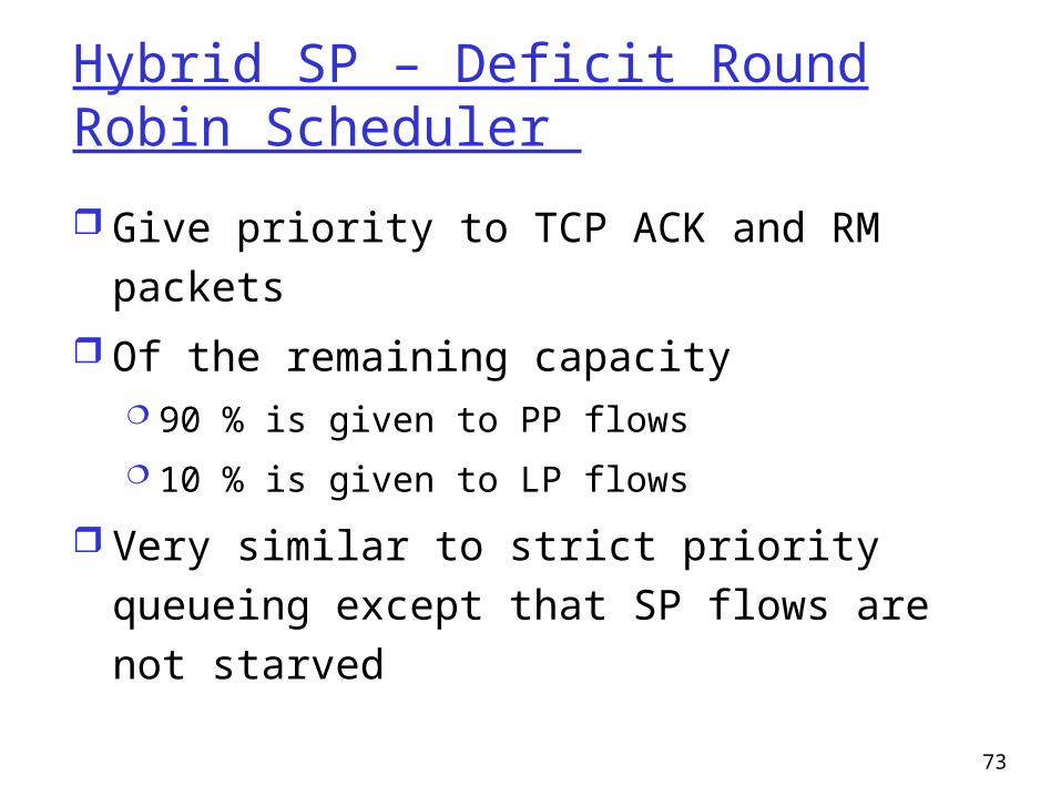
Hybrid SP – Deficit Round Robin Scheduler

Give priority to TCP ACK and RM packets

Of the remaining capacity 90 % is given to PP flows

10 % is given to LP flows

Very similar to strict priority queueing except that SP flows are not starved

74

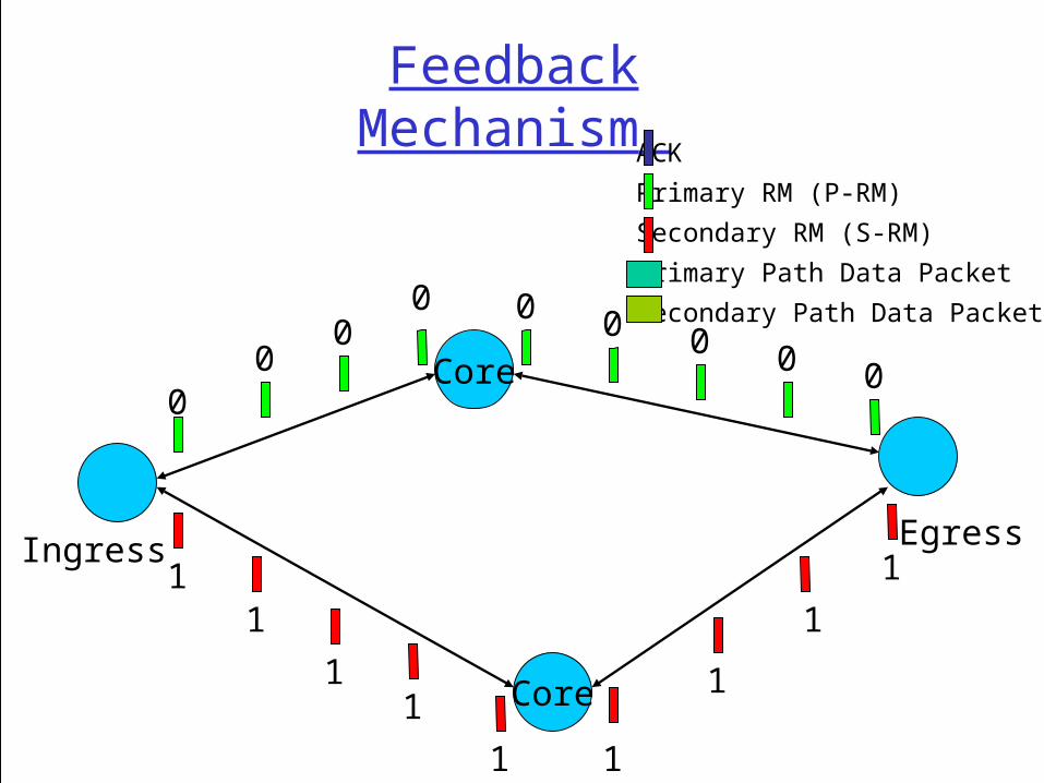
Feedback Mechanism

Core

ACK

Primary RM (P-RM)

Secondary RM (S-RM)

Primary Path Data Packet

Secondary Path Data Packet

Core

Ingress Egress

0

0

0

0

0

0

0

0

Gold Silver Bronze

0

0

1

0

1

0

1

Gold Silver Bronze

0

1

75

Feedback Mechanism

Core

ACK

Primary RM (P-RM)

Secondary RM (S-RM)

Primary Path Data Packet

Secondary Path Data Packet

Core

Ingress Egress

0

1

0

1

0

1

0

1

0

1

0

1

0

1

0

11

0

76

Rate Control • When the Ingress Node receives the congestion

information about the path, it will invoke an AIMD (Additive Increase Multiplicative Decrease) algorithm to compute the ATR (Allowed Transmission Rate) of the corresponding path.

ATR: Allowed Transmission Rate

RDF: Rate Decrease Factor

RIF: Rate Increase Factor

MTR: Minimum Transmission Rate

PTR: Peak Transmission Rate

77

Traffic Splitting

• When a new flow arrives at an ingress router, a decision on how to forward the packets of this new flow needs to be made.

• We compute the DPP and DSP delay estimates for the PP and SP queues at the Edge Node, respectively.

• Then calculate and update dn that is averaged (smoothed) difference, DPP - DSP, at the epoch of the nth packet arrival

Traffic Splitting Units Per-egress queuing Per-class queuing

PP Queue

SP Queue

Silver Queue

Bronze Queue

Gold Queue

RM + TCP ACK

DPP

DPPPP Queue

SP Queue

DSP

DSP

+

-

+

-

Incoming FlowsFor Destination 1

Incoming FlowsFor Destination 2

AIMD

78

Random Early Reroute

• By using the updated dn value, we decide whether to assign this new flow to PP or SP:

• Assign the new flow to PP with probability (1-p(dn))

• Assign the new flow to SP with probability (p(dn))

• We call this policy as Random Early Reroute (RER). It is used for controlling the delay difference of queues of PP and SP

• This policy gives priority to PP over SP on the edge nodes.

79

Simulation SettingThree Node Network Topology

Core 2

Core 3Core 1

Edge 2

Edge 1 Edge 3

• Flow size dist. = Bounded Pareto

• Flow interarrival dist. = Poisson

• Total traffic from each node = 70 Mb/s

• Speed of core links = 50 Mb/s

80

Simulation Parameters Mesh Network Topology

s f

la

s j

d e

c h

c l

ny

d c

s l

d a

h s

a t

• This topology and the traffic demand matrix T[i,j] are used from the data given in www.fictitious.org/omp.

• Each link is bi-directional and has 45 Mb/s capacity in both directions except the links between de-ch and ch-cl have 90 Mb/s capacity in both directions.

90Mb/s

90Mb/s

45Mb/s

81

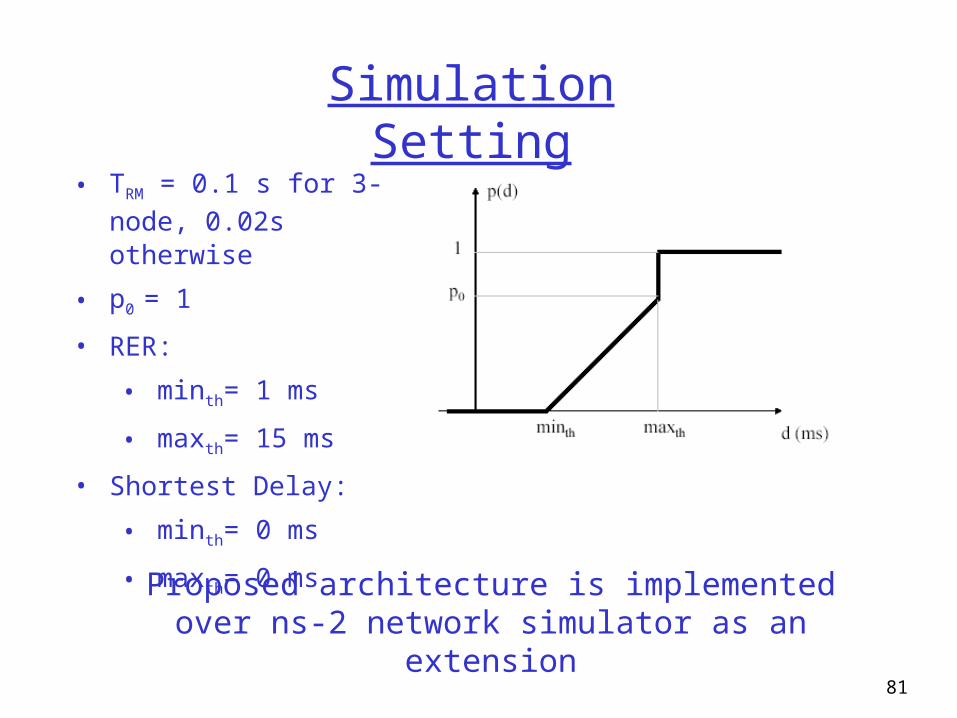
Simulation Setting

• TRM = 0.1 s for 3-node, 0.02s otherwise

• p0 = 1

• RER:

• minth= 1 ms

• maxth= 15 ms

• Shortest Delay:

• minth= 0 ms

• maxth= 0 ms

Proposed architecture is implemented over ns-2 network simulator as an extension

83

Results - 3 nodes

84

Results – Large topology

85

Triangle Effect – 3 Nodes

86

Large Topology