1 the disturbance term in logarithmic models thus far, nothing has been said about the disturbance...

1

THE DISTURBANCE TERM IN LOGARITHMIC MODELS

Thus far, nothing has been said about the disturbance term in nonlinear regression models.

uX

Y 21

XZ

1

uZY 21

2

For the regression results in a linearized model to have the desired properties, the disturbance term in the transformed model should be additive and it should satisfy the regression model conditions.


uX

Y 21

XZ

1

uZY 21

3

To be able to perform the usual tests, it should be normally distributed in the transformed model.


uX

Y 21

XZ

1

uZY 21

4

In the case of the first example of a nonlinear model, there was no problem. If the disturbance term had the required properties in the original model, it would have them in the regression model. It has not been affected by the transformation.

uX

Y 21

XZ

1

uZY 21


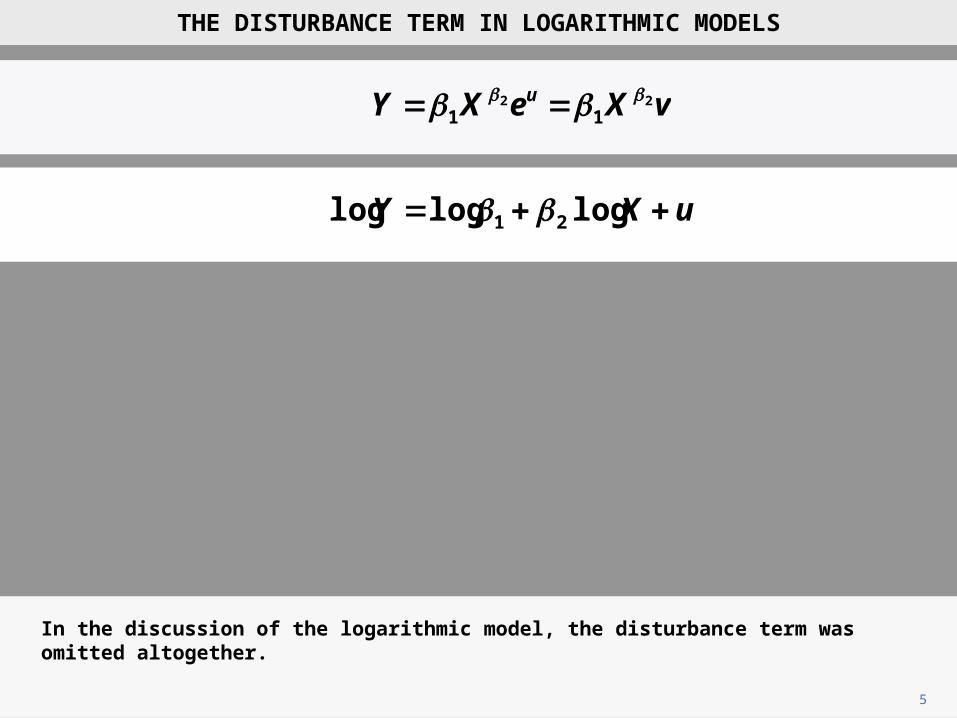
uXY logloglog 21

5

In the discussion of the logarithmic model, the disturbance term was omitted altogether.


vXeXY u 2211

6


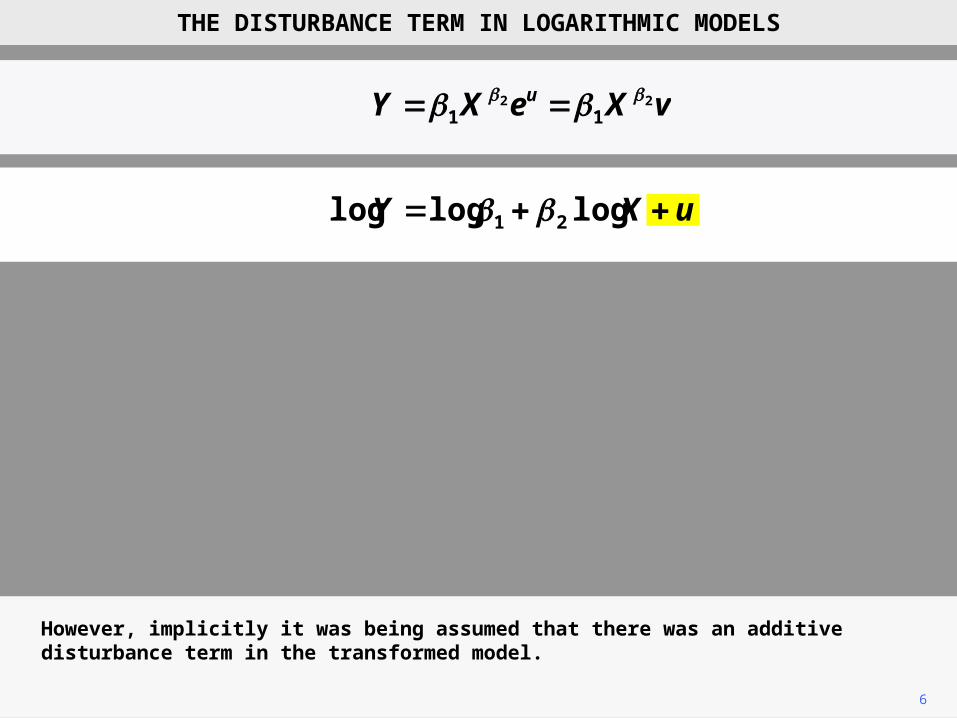
However, implicitly it was being assumed that there was an additive disturbance term in the transformed model.

vXeXY u 2211

uXY logloglog 21

7


For this to be possible, the random component in the original model must be a multiplicative term, eu.

vXeXY u 2211

uXY logloglog 21

8


We will denote this multiplicative term v.

vXeXY u 2211

uXY logloglog 21

9


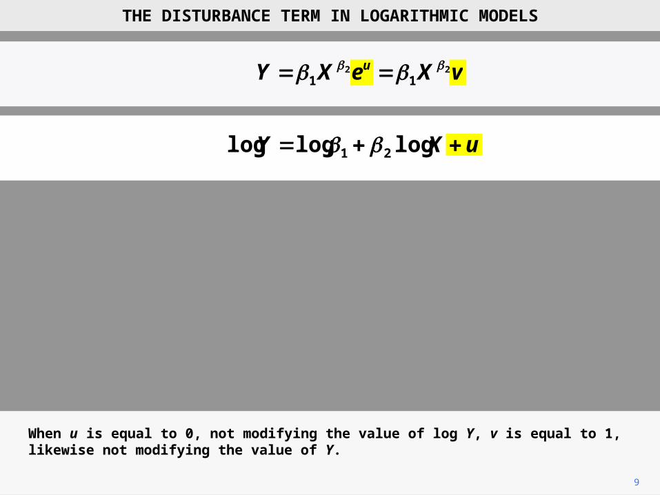
When u is equal to 0, not modifying the value of log Y, v is equal to 1, likewise not modifying the value of Y.

vXeXY u 2211

uXY logloglog 21

10


Positive values of u correspond to values of v greater than 1, the random factor having a positive effect on Y and log Y. Likewise negative values of u correspond to values of v between 0 and 1, the random factor having a negative effect on Y and log Y.

vXeXY u 2211

uXY logloglog 21

0.00

0.05

0.10

0.15

0.20

0.25

0.30

0.35

0.40

0.45

0 1 2 3 4 5 6 7 8 9 10 11 12 13 14 15 16v

f(v)

11

Besides satisfying the regression model conditions, we need u to be normally distributed if we are to perform t tests and F tests.


uXY logloglog 21

vXeXY u 2211

0.00

0.05

0.10

0.15

0.20

0.25

0.30

0.35

0.40

0.45

0 1 2 3 4 5 6 7 8 9 10 11 12 13 14 15 16v

f(v)

12


uXY logloglog 21

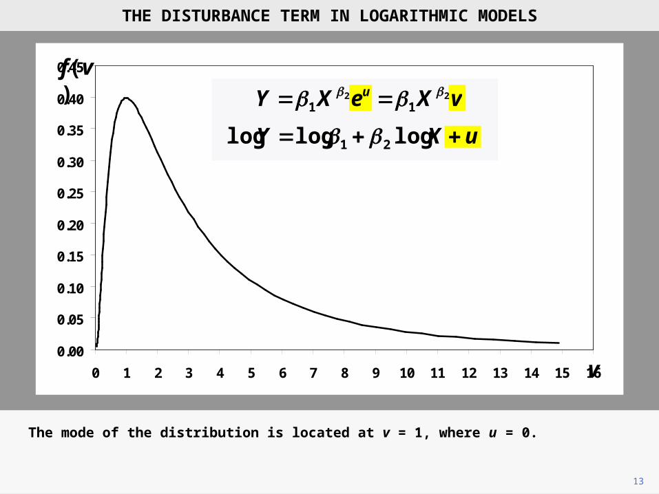
This will be the case if v has a lognormal distribution, shown above.

vXeXY u 2211

0.00

0.05

0.10

0.15

0.20

0.25

0.30

0.35

0.40

0.45

0 1 2 3 4 5 6 7 8 9 10 11 12 13 14 15 16v

f(v)

13


uXY logloglog 21

vXeXY u 2211

The mode of the distribution is located at v = 1, where u = 0.

0.00

0.05

0.10

0.15

0.20

0.25

0.30

0.35

0.40

0.45

0 1 2 3 4 5 6 7 8 9 10 11 12 13 14 15 16v

f(v)

14


The same multiplicative disturbance term is needed in the semilogarithmic model.

veeeY XuX 2211

uXY 21loglog

0.00

0.05

0.10

0.15

0.20

0.25

0.30

0.35

0.40

0.45

0 1 2 3 4 5 6 7 8 9 10 11 12 13 14 15 16v

f(v)

15


veeeY XuX 2211

uXY 21loglog

Note that, with this distribution, one should expect a small proportion of observations to be subject to large positive random effects.

16

Here is the scatter diagram for earnings and schooling using Data Set 21. You can see that there are several outliers, with the four most extreme highlighted.


-20

0

20

40

60

80

100

120

0 1 2 3 4 5 6 7 8 9 10 11 12 13 14 15 16 17 18 19 20

Ho

url

y ea

rnin

gs

($)

Years of schooling (highest grade completed)

17

Here is the scatter diagram for the semilogarithmic model, with its regression line. The same four observations remain outliers, but they do not appear to be so extreme.


0

1

2

3

4

5

0 1 2 3 4 5 6 7 8 9 10 11 12 13 14 15 16 17 18 19 20

Lo

gar

ith

m o

f h

ou

rly

earn

ing

s

Years of schooling (highest grade completed)

18

The histogram above compares the distributions of the residuals from the linear and semi-logarithmic regressions. The distributions have been standardized, that is, scaled so that they have standard deviation equal to 1, to make them comparable.

0–1–2–3 1 2 3


0

20

40

60

80

100

120

140

160

180

200

Linear Semilogarithmic

19

0–1–2–3 1 2 3


0

20

40

60

80

100

120

140

160

180

200


It can be shown that if the disturbance term in a regression model has a normal distribution, so will the residuals.

20

0–1–2–3 1 2 3


0

20

40

60

80

100

120

140

160

180

200


It is obvious that the residuals from the semilogarithmic regression are approximately normal, but those from the linear regression are not. This is evidence that the semi-logarithmic model is the better specification.

21

What would happen if the disturbance term in the logarithmic or semilogarithmic model were additive, rather than multiplicative?


uXY 21

22

If this were the case, we would not be able to linearize the model by taking logarithms. There is no way of simplifying log(b1Xb + u). We should have to use some nonlinear regression technique.

uXY 21

)log(log 21 uXY

2


Copyright Christopher Dougherty 2012.

These slideshows may be downloaded by anyone, anywhere for personal use.

Subject to respect for copyright and, where appropriate, attribution, they may be

used as a resource for teaching an econometrics course. There is no need to

refer to the author.

The content of this slideshow comes from Section 4.2 of C. Dougherty,

Introduction to Econometrics, fourth edition 2011, Oxford University Press.

Additional (free) resources for both students and instructors may be

downloaded from the OUP Online Resource Centre

http://www.oup.com/uk/orc/bin/9780199567089/.

Individuals studying econometrics on their own who feel that they might benefit

from participation in a formal course should consider the London School of

Economics summer school course

EC212 Introduction to Econometrics

http://www2.lse.ac.uk/study/summerSchools/summerSchool/Home.aspx

or the University of London International Programmes distance learning course

EC2020 Elements of Econometrics

www.londoninternational.ac.uk/lse.

2012.11.03

http://www.oup.com/uk/orc/bin/9780199567089/

http://www2.lse.ac.uk/study/summerSchools/summerSchool/Home.aspx

1 the disturbance term in logarithmic models thus far, nothing has been said about the disturbance...

Documents