1 simulating underwater sensor networks and...
TRANSCRIPT

1
SIMULATING UNDERWATER SENSOR NETWORKS AND ROUTINGALGORITHMS IN MATLAB
by
Michael J. O’Rourke
A Thesis Submitted to the
Office of Research and Graduate Studies
In Partial Fulfillment of the
Requirements for the Degree of
MASTER OF SCIENCE
School of Engineering and Computer ScienceEngineering Science
University of the PacificStockton, California
2013

2
SIMULATING UNDERWATER SENSOR NETWORKS AND ROUTINGALGORITHMS IN MATLAB
by
Michael J. O’Rourke
APPROVED BY:
Thesis Advisor: Elizabeth Basha, Ph.D.
Committee Member: Carrick Detweiler, Ph.D.
Committee Member: Ken Hughes, Ph.D.
Department Chairperson: Jennifer Ross, Ph.D.
Interim Dean of Graduate Studies: Bhaskara R. Jasti, Ph.D.

3
DEDICATION
This work is dedicated my family, friends, thesis committee, and the staff of the University
of the Pacific School of Engineering and Computer Science. The endless support I’ve
received from all parties allowed me to complete this and without their help I’d have given
up long ago.

4
ACKNOWLEDGMENTS
I’d like to acknowledge my committee: Dr. Basha, Dr. Detweiler, and Dr. Hughes. Dr.
Basha, chair of the committee and my advisor, regularly offered keen insight and gave me
freedom to approach this my own way. Her patience has been admirable, and I appreciate
that I had the opportunity to work with her. Dr. Detweiler challenged me to carry this
project forward and helped me identify ways to be more productive in development. Dr.
Hughes and Dr. Detweiler helped me understand where weak points have been, and with
the members of my committee I believe I’ve done something to be proud of.
I would also like to thank the National Science Foundation for supporting the research
(CSR #1217400 and CSR #1217428) as well as the School of Engineering and Computer
Science.
I’d also like to thank my friend Adam Yee. Whether it was talking through my ideas
late at night, explaining the system in different ways, or simply justifying my decisions,
Adam was always available. With his assistance, I was able to keep my goals realistic and
intentions clear.

5
Simulating Underwater Sensor Networks and Routing Algorithms in MATLAB
Abstract
by Michael J. O’Rourke
University of the Pacific
2013
Underwater networks are a field that has been gathering attention. Land-based meth-
ods of network construction from discovery to advanced routing are all well established.
Due to the unique constraints of operating in an underwater environment, many of these
tried-and-true approaches need modification if they function at all. Peer discovery and low-
level networking have been dealt with by previous research. In this thesis we describe and
evaluate eight possible routing schemes with different system-knowledge requirements. We
show that with a minimal set of information it is possible to achieve near-optimal results
with energy costs considerably lower than centralized optimal algorithms.
We demonstrate this by constructing and evaluating a custom simulation environment
in MATLAB. This is implemented in a mixed procedural and array-centric approach. Sim-
ulated networks are structured on a line topology. All nodes a spaced along the horizontal
axis at a random depth. It is assumed that neighbor-discovery has been completed before
the simulation starts, and all nodes have access to a global list of connected neighbors. We
6
demonstrate the effectiveness of distributed algorithms in an ideal environment, leading to
the conclusion that near-optimal results can be achieved with local information only.

7
TABLE OF CONTENTS
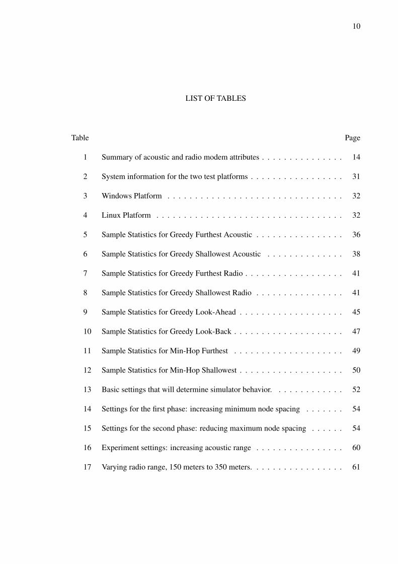
LIST OF TABLES . . . . . . . . . . . . . . . . . . . . . . . . . . . . . . . . . . . . . . 10
LIST OF FIGURES . . . . . . . . . . . . . . . . . . . . . . . . . . . . . . . . . . . . . 11
CHAPTER
1 Introduction . . . . . . . . . . . . . . . . . . . . . . . . . . . . . . . . . . . . 14
1.1 The Problem and Approach . . . . . . . . . . . . . . . . . . . . . . 15
1.2 Overview of Experiments . . . . . . . . . . . . . . . . . . . . . . . . 18
1.3 Thesis Outline . . . . . . . . . . . . . . . . . . . . . . . . . . . . . . 19
2 Related Work . . . . . . . . . . . . . . . . . . . . . . . . . . . . . . . . . . . 20
2.1 Wireless Underwater Networks . . . . . . . . . . . . . . . . . . . . 20
2.2 Multimodal Communication . . . . . . . . . . . . . . . . . . . . . . 21
3 The Simulation Environment . . . . . . . . . . . . . . . . . . . . . . . . . . 23
3.1 MATLAB . . . . . . . . . . . . . . . . . . . . . . . . . . . . . . . . . 23
3.1.1 Object Oriented Environment. . . . . . . . . . . . . . . . 24
3.1.2 Procedural Environment. . . . . . . . . . . . . . . . . . . 26
3.2 Simulation Structure . . . . . . . . . . . . . . . . . . . . . . . . . . 28
3.3 Environment Performance Metrics . . . . . . . . . . . . . . . . . . 30
3.3.1 How Time is Measured. . . . . . . . . . . . . . . . . . . . 30
3.3.2 How Memory is Measured. . . . . . . . . . . . . . . . . . 30
3.4 Performance Results . . . . . . . . . . . . . . . . . . . . . . . . . . 31
3.4.1 Environment Performance. . . . . . . . . . . . . . . . . . 31
4 Algorithms Implemented . . . . . . . . . . . . . . . . . . . . . . . . . . . . . 33
4.1 Acoustic-Centric Algorithms . . . . . . . . . . . . . . . . . . . . . . 34
8
4.1.1 Greedy Furthest Acoustic. . . . . . . . . . . . . . . . . . 34
4.1.2 Greedy Shallowest Acoustic. . . . . . . . . . . . . . . . . 37
4.2 Radio-Centric Algorithms . . . . . . . . . . . . . . . . . . . . . . . 38
4.2.1 Greedy Furthest Radio. . . . . . . . . . . . . . . . . . . . 39
4.2.2 Greedy Shallowest Radio. . . . . . . . . . . . . . . . . . 41
4.2.3 Greedy Look-Ahead. . . . . . . . . . . . . . . . . . . . . 42
4.2.4 Greedy Look-Back. . . . . . . . . . . . . . . . . . . . . . 45
4.2.5 Min-Hop Furthest. . . . . . . . . . . . . . . . . . . . . . . 47
4.2.6 Min-Hop Shallowest. . . . . . . . . . . . . . . . . . . . . 49
5 Experiments and Results . . . . . . . . . . . . . . . . . . . . . . . . . . . . . 51
5.1 Experiments . . . . . . . . . . . . . . . . . . . . . . . . . . . . . . . 51
5.1.1 Basic System, All Algorithms. . . . . . . . . . . . . . . . 51
5.1.2 Varying Node Placement. . . . . . . . . . . . . . . . . . . 54
5.1.3 Varying Acoustic Range, Fixed Radio Range. . . . . . . 60
5.1.4 Varying Radio Range, Fixed Acoustic Range. . . . . . . 61
5.2 Discussion . . . . . . . . . . . . . . . . . . . . . . . . . . . . . . . . 62
6 Conclusions . . . . . . . . . . . . . . . . . . . . . . . . . . . . . . . . . . . . 66
6.1 Summary In Brief . . . . . . . . . . . . . . . . . . . . . . . . . . . . 66
6.2 Contributions . . . . . . . . . . . . . . . . . . . . . . . . . . . . . . . 67
6.3 Future Work . . . . . . . . . . . . . . . . . . . . . . . . . . . . . . . 68
REFERENCES . . . . . . . . . . . . . . . . . . . . . . . . . . . . . . . . . . . . . . . 69
APPENDICES
A. MATLAB CODE . . . . . . . . . . . . . . . . . . . . . . . . . . . . . . . . . 72
A.1 Initializers . . . . . . . . . . . . . . . . . . . . . . . . . . . . . . . . 72
9
A.2 Main Body . . . . . . . . . . . . . . . . . . . . . . . . . . . . . . . . 76
A.3 Helper Functions . . . . . . . . . . . . . . . . . . . . . . . . . . . . 81
10
LIST OF TABLES
Table Page
1 Summary of acoustic and radio modem attributes . . . . . . . . . . . . . . . 14
2 System information for the two test platforms . . . . . . . . . . . . . . . . . 31
3 Windows Platform . . . . . . . . . . . . . . . . . . . . . . . . . . . . . . . . 32
4 Linux Platform . . . . . . . . . . . . . . . . . . . . . . . . . . . . . . . . . . 32
5 Sample Statistics for Greedy Furthest Acoustic . . . . . . . . . . . . . . . . 36
6 Sample Statistics for Greedy Shallowest Acoustic . . . . . . . . . . . . . . 38
7 Sample Statistics for Greedy Furthest Radio . . . . . . . . . . . . . . . . . . 41
8 Sample Statistics for Greedy Shallowest Radio . . . . . . . . . . . . . . . . 41
9 Sample Statistics for Greedy Look-Ahead . . . . . . . . . . . . . . . . . . . 45
10 Sample Statistics for Greedy Look-Back . . . . . . . . . . . . . . . . . . . . 47
11 Sample Statistics for Min-Hop Furthest . . . . . . . . . . . . . . . . . . . . 49
12 Sample Statistics for Min-Hop Shallowest . . . . . . . . . . . . . . . . . . . 50
13 Basic settings that will determine simulator behavior. . . . . . . . . . . . . 52
14 Settings for the first phase: increasing minimum node spacing . . . . . . . 54
15 Settings for the second phase: reducing maximum node spacing . . . . . . 54
16 Experiment settings: increasing acoustic range . . . . . . . . . . . . . . . . 60
17 Varying radio range, 150 meters to 350 meters. . . . . . . . . . . . . . . . . 61

11
LIST OF FIGURES
Figure Page
1 Picture of an AquaNode [5] . . . . . . . . . . . . . . . . . . . . . . . . . . . 15
2 AquaNodes finding a radio path . . . . . . . . . . . . . . . . . . . . . . . . . 17
3 Chart of Simulation Structure . . . . . . . . . . . . . . . . . . . . . . . . . . 27
4 Graph of Start and End positions for Greedy Furthest Acoustic . . . . . . . 36
5 Graph of Start and End positions for Greedy Shallowest Acoustic . . . . . 39
6 Graph of Start and End positions for Greedy Furthest Radio . . . . . . . . . 40
7 Graph of Start and End positions for Greedy Shallowest Radio . . . . . . . 42
8 Graph of Start and End positions for Greedy Look-Ahead . . . . . . . . . . 43
9 Graph of Start and End positions for Greedy Look-Back . . . . . . . . . . . 47
10 Graph of Start and End positions for Min-Hop Furthest . . . . . . . . . . . 49
11 Graph of Start and End positions for Min-Hop Shallowest . . . . . . . . . . 50
12 Graph of Start and End positions for Greedy Furthest Acoustic . . . . . . . 53
13 Graph of Energy Consumed by Four Algorithms . . . . . . . . . . . . . . . 53
14 The Effect Separating Nodes Further on Distance . . . . . . . . . . . . . . . 55
15 The Effect on 50 Nodes Being Separated Further . . . . . . . . . . . . . . . 56
16 The Effect Separating Nodes Further on Energy Use . . . . . . . . . . . . . 56
17 The Effect on Power Consumption Increased Separation has on 50 Nodes . 57
18 The Effect Placing Nodes Closer Together on Distance . . . . . . . . . . . 57
12
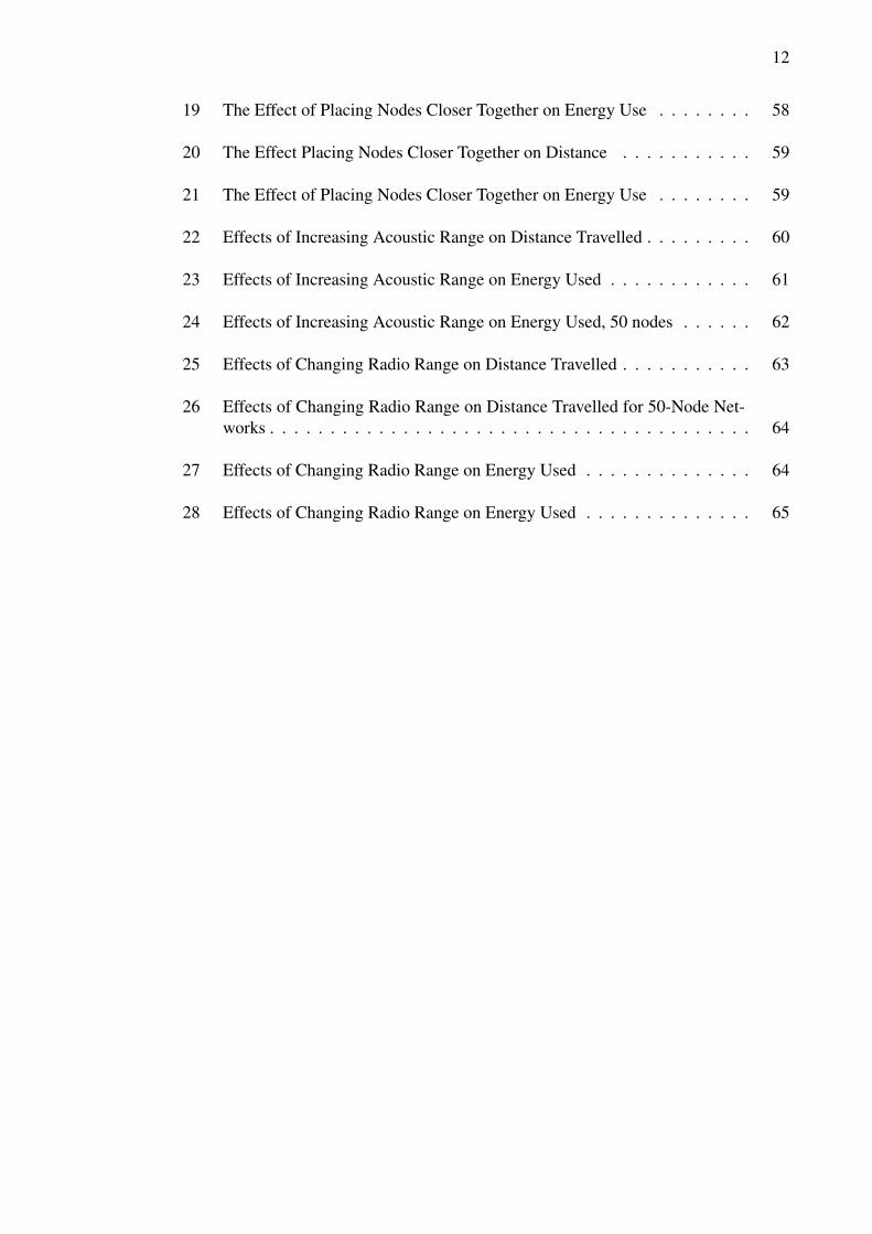
19 The Effect of Placing Nodes Closer Together on Energy Use . . . . . . . . 58
20 The Effect Placing Nodes Closer Together on Distance . . . . . . . . . . . 59
21 The Effect of Placing Nodes Closer Together on Energy Use . . . . . . . . 59
22 Effects of Increasing Acoustic Range on Distance Travelled . . . . . . . . . 60
23 Effects of Increasing Acoustic Range on Energy Used . . . . . . . . . . . . 61
24 Effects of Increasing Acoustic Range on Energy Used, 50 nodes . . . . . . 62
25 Effects of Changing Radio Range on Distance Travelled . . . . . . . . . . . 63
26 Effects of Changing Radio Range on Distance Travelled for 50-Node Net-works . . . . . . . . . . . . . . . . . . . . . . . . . . . . . . . . . . . . . . . . 64
27 Effects of Changing Radio Range on Energy Used . . . . . . . . . . . . . . 64
28 Effects of Changing Radio Range on Energy Used . . . . . . . . . . . . . . 65
13
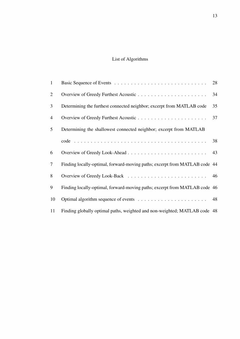
List of Algorithms
1 Basic Sequence of Events . . . . . . . . . . . . . . . . . . . . . . . . . . . . 28
2 Overview of Greedy Furthest Acoustic . . . . . . . . . . . . . . . . . . . . . 34
3 Determining the furthest connected neighbor; excerpt from MATLAB code 35
4 Overview of Greedy Furthest Acoustic . . . . . . . . . . . . . . . . . . . . . 37
5 Determining the shallowest connected neighbor; excerpt from MATLAB
code . . . . . . . . . . . . . . . . . . . . . . . . . . . . . . . . . . . . . . . . 38
6 Overview of Greedy Look-Ahead . . . . . . . . . . . . . . . . . . . . . . . . 43
7 Finding locally-optimal, forward-moving paths; excerpt from MATLAB code 44
8 Overview of Greedy Look-Back . . . . . . . . . . . . . . . . . . . . . . . . 46
9 Finding locally-optimal, forward-moving paths; excerpt from MATLAB code 46
10 Optimal algorithm sequence of events . . . . . . . . . . . . . . . . . . . . . 48
11 Finding globally optimal paths, weighted and non-weighted; MATLAB code 48
14
Chapter 1: Introduction
Just over 70% of the planet is covered in water. Very little of that is explored, and
we likely understand even less. One way researchers are approaching this is by innovating
with underwater robots and networks. In this thesis we define a simulation environment that
describes an underwater network where nodes are able to efficiently surface to use radio
communication. Using this environment we determine paths for radio communication on
a line topology in a multimodal system. We implement a total of eight different algorithms
to facilitate decisions about communication.
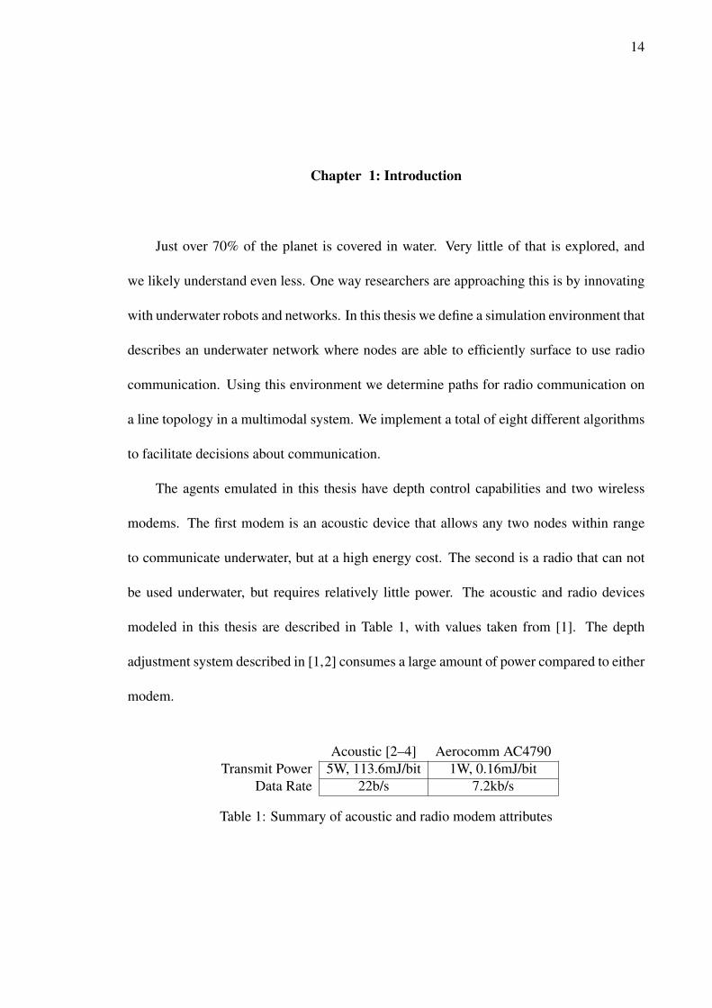
The agents emulated in this thesis have depth control capabilities and two wireless
modems. The first modem is an acoustic device that allows any two nodes within range
to communicate underwater, but at a high energy cost. The second is a radio that can not
be used underwater, but requires relatively little power. The acoustic and radio devices
modeled in this thesis are described in Table 1, with values taken from [1]. The depth
adjustment system described in [1,2] consumes a large amount of power compared to either
modem.
Acoustic [2–4] Aerocomm AC4790Transmit Power 5W, 113.6mJ/bit 1W, 0.16mJ/bit
Data Rate 22b/s 7.2kb/s
Table 1: Summary of acoustic and radio modem attributes
15
Our primary concern is then: how do we pass a message across the network in an
efficient way? As shown in [1, 5], there is a clear cutoff of when the cost of rising will
be less than the cost of forwarding a large message acoustically. In reference to that, the
algorithms defined in Chapter 4 provide a method of selecting who will rise and participate
in radio-message forwarding. We determine that distributed algorithms using only local
information can perform at or near the level globally optimal algorithms for determining
members of the radio path. This thesis contributes to the field of underwater networks
by demonstrating the effectiveness of greedy routing schemes that use locally available
information, and by providing a simulator in which they can be tested.
1.1 The Problem and Approach
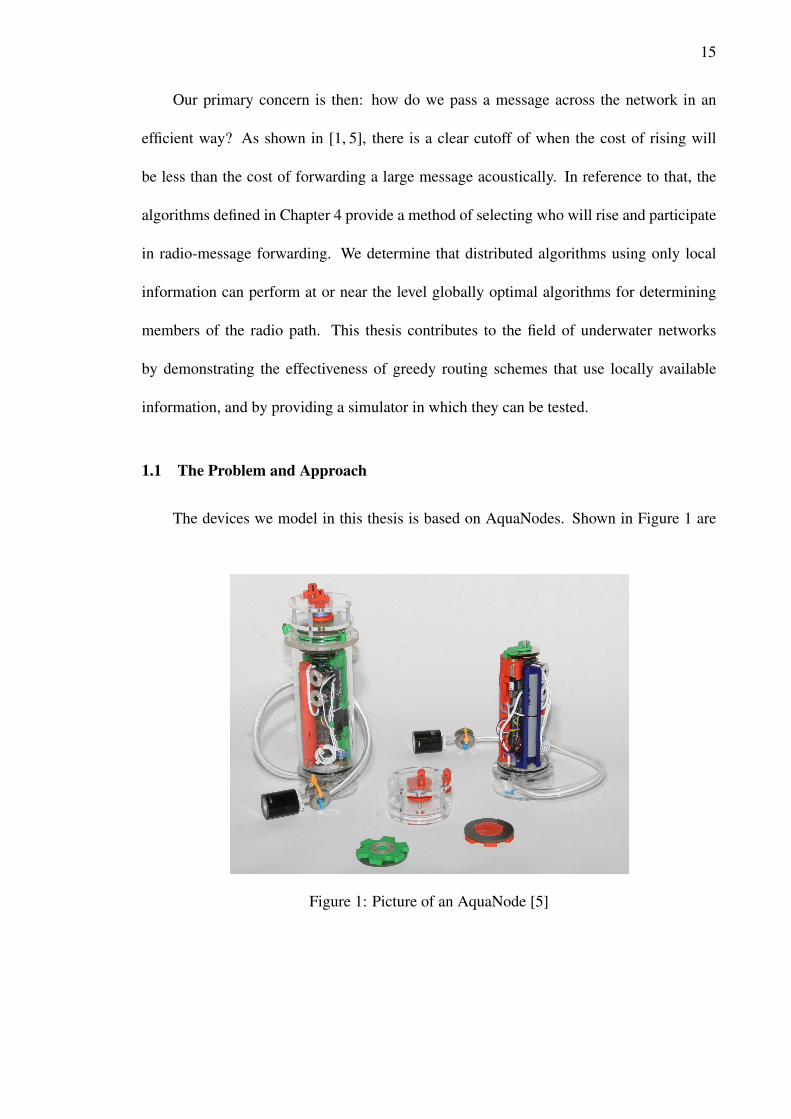
The devices we model in this thesis is based on AquaNodes. Shown in Figure 1 are
Figure 1: Picture of an AquaNode [5]
16
two AquaNodes, one complete in its water-proof casing and one exposed. In addition to
the modems mentioned earlier, these devices have multiple processors, a range of sensors,
and a depth control system. We simplify this by assuming the more power-consuming
processor is always on; the sensors are not implemented within this thesis.
The radio on each system is not usable underwater. As presented in Table 1, radio
communication is both faster and less expensive. In our context, the problem with radio
communication is the cost of surfacing; using the depth adjustment system. The average
cost of motion, ascending or descending, is determined to be 15000mJ/m or 15 Joules/me-
ter. All other energy costs are in the mJ, or in some cases µJ range. Rising then dominates
cost until message size increases above a threshold.
We assume in this thesis that a large collection of data, well exceeding the point at
which sending it all acoustically is more expensive than the average cost of rising, is ready
to be forwarded. It is thus our task to determine which nodes in the network will surface to
participate in forwarding radio messages.
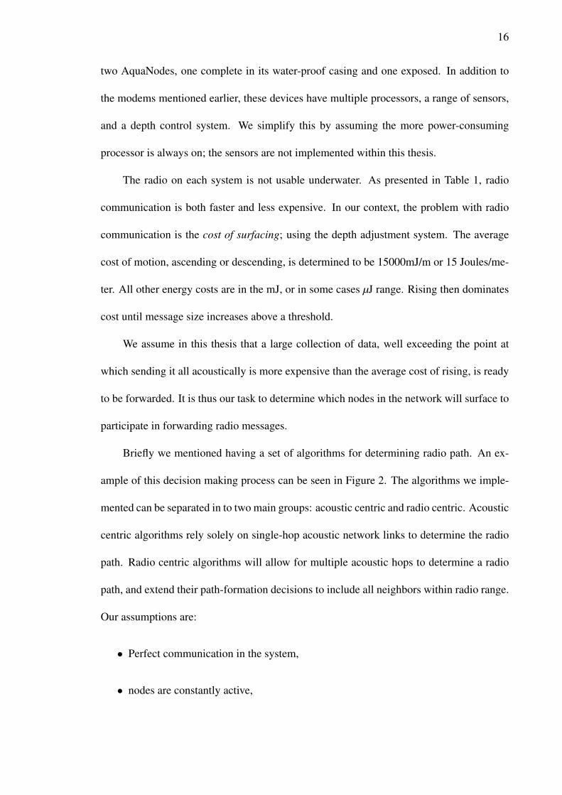
Briefly we mentioned having a set of algorithms for determining radio path. An ex-
ample of this decision making process can be seen in Figure 2. The algorithms we imple-
mented can be separated in to two main groups: acoustic centric and radio centric. Acoustic
centric algorithms rely solely on single-hop acoustic network links to determine the radio
path. Radio centric algorithms will allow for multiple acoustic hops to determine a radio
path, and extend their path-formation decisions to include all neighbors within radio range.
Our assumptions are:
• Perfect communication in the system,
• nodes are constantly active,
17
Figure 2: AquaNodes finding a radio path
18
• limitless power for each node,
• peer discovery is completed before the simulation starts,
• and that nodes will only move vertically.
We then seek to determine the best method of choosing a radio path. All of the algorithms
are described in detail in Chapter 4, and the experiments we conduct to determine the best
methods are discussed at length in Chapter 5.
1.2 Overview of Experiments
There are a total of four basic experiments for testing network models, and two for
characterizing the environment. For characterizing the environment we run a single-algorithm
at default system settings on two different systems. The first system is running Windows
XP, and demonstrates performance on previous generation systems. The second system is
running Ubuntu Linux and has much higher capabilities (memory, processing, etc.). The
systems and experiments are presented in further detail in 3.4.
The four algorithm/model tests are: all default settings, default settings but changing
node-placement rules, default settings and changing acoustic range, and default settings
while changing radio range. The first experiment details typical behavior of the system
across all algorithms. The second experiment explains the effect of node placement on
algorithm performance.
In acoustic-range testing, the range is set to the minimum placement between nodes
and then expanded several times beyond maximum distance between neighbors. A similar
track is followed for radio-range testing. Radio testing constrains itself to default acoustic
range, expands out beyond to typical range, and is finally set to several times typical range.

19
All of the range testing relies on typical node placement which has a random aspect to it,
but guarantees that all nodes have at least two acoustic neighbors (and at most six).
The basic all-algorithm test and node placement tests are run on all algorithms. The
range tests are run on a subset including Greedy Furthest Radio (4.2.1), Greedy Shallowest
Radio (4.2.2), Greedy Look-Ahead (4.2.3), and Min-Hop Shallowest (4.2.6).
1.3 Thesis Outline
This thesis is composed of five additional chapters. In chapter 2 we discuss prelimi-
nary work in underwater networks. With chapter 3 we describe and characterize the custom
simulation environment we created to support this work. The inner workings of the environ-
ment are discussed there, and data are presented that describes environment performance
on different platforms. Going to chapter 4 all eight algorithms are described, characterized
over one-thousand unique topologies on sizes ranging from 25 to 100 nodes. Basic statis-
tics are presented as well as sample graphs demonstrating the behavior of each algorithm
on a ten-node network.
Chapter 5 describes all experiments at length and presents the results. Concluding
remarks are offered in 6, and followed by an appendix containing the code for all algorithms
and the environment.
20
Chapter 2: Related Work
Our system takes advantage of multiple communication methods to within an under-
water network. We develop an idealized simulation environment that eliminates many of
the challenges of networking, and assume peer discovery has already been completed. As
we function on an abstract level rather than handling specific issues of implementing net-
worked systems, we draw from algorithmic studies and rely on values from work done with
physical systems.
2.1 Wireless Underwater Networks
It is common for sensor networks to rely on gateway nodes to handle large amounts of
data over long ranges [6–8]. An example of this is the SeaWeb [9] system. SeaWeb used
nodes at the surface to support communication with the outside world, and for localization
within its own network via GPS. Research has been done that demonstrates the practical
nature of using gateways in underwater networks [10]. Zhou et al. used linear programming
to optimize the placement of these gateways to minimize power and delay [11].
What could be considered a flaw of these surface-gateway systems is that the acoustic
modem limits communication. All nodes must transmit acoustically to have data forwarded
out of the underwater part of the network. This places a natural limit on the rate at which
data can be extricated; in an ideal system data could be retrieved at the maximum rate of the
modem, but a real system would face packet loss. To mitigate this problem, work has been
21
done to introduce underwater vehicles to these systems and retrieve data as policy dictates.
These vehicles collect data along a path and occasionally rise to send data via radio [1,12].
The system we implement is different in that each node is capable of surfacing to
send its own data or relay transmissions from its neighbors. Issues associated with acoustic
gateways are removed in this scenario. The drawback of this approach is that nodes could
be moved from their correct location for sensing, and the power-cost of rising needs to
be factored in to routing decisions. For this paper we explore different approaches for
determining radio paths on a line topology, attempting to minimizing energy consumption.
To that end we implement optimal path finding algorithms, examine greedy approaches,
and compare the results of these. The greedy approaches are similar to greedy geographic
routing in land-based systems which are near-optimal in dense networks, and varying im-
plementations have been demonstrated to improve performance in challenging and dy-
namic environments [13, 14]. Given the high performance of greedy methods in land-
environments, we are motivated to explore their loose analogues in the underwater arena.
2.2 Multimodal Communication
Land-based sensor networks have been exploring multimodal communication for years.
For example, in [15,16] the authors describe gateway devices that combine short range and
long range communication. Just like underwater systems, the in-network modem and gate-
ways become choke-points. Chen and Ma describe MEMOSEN [6], and demonstrate the
effectiveness of mobile multimodal systems in sensor networks. MEMOSEN uses cluster-
ing to structure networks. Within a cluster, a low-power radio such as bluetooth is used to
facilitate data transfer. Between clusters and out of the system use a longer-range/higher-
power device, with designated gateways.

22
Our system does not deal with gateways, and intentionally allows for any node to rise
and send its own data. In that regard, we see the idea of opportunistic mode changes in [17].
Chumkamon et al. explore vehicular networks that arbitrate between modems based on
convenience and availability. We see the greatest connection with our own research by
combining the works of [18] and [6]. Lin et al. use a decentralized system of low-power
communication coordinators to determine which network agents will use higher-power de-
vices to send or relay data. MEMOSEN describes a distributed mobile system without
strict rules on who will engage in high-throughput communication.
We differ from and extend these by: moving to underwater systems, changing com-
munication parameters (i.e., our high-throughput is our low-power device), and we have a
set decision policy for determining who will participate in “elevated” communication.
23
Chapter 3: The Simulation Environment
In this chapter we discuss the software we developed to simulate aquatic networks.
We start be explaining why we chose to develop in MATLAB. Then we discuss the two
versions of the simulator we implemented, an object-oriented approach and a procedural
approach respectively. Originally we used the object oriented approach, but abandoned it
in favor of the procedural approach due to the difficulties introduced into the debug process
that were not relevant to this thesis. Then we detail the basic structure of the system,
define performance metrics of the environment and models, and close with a discussion of
simulation performance on two platforms.
3.1 MATLAB
The environment is implemented as a set of MATLAB scripts and functions. There
are a several benefits to this decision including: ease of development, industry acceptance,
native support for large numbers, and efficient storage and handling of large data sets.
Using a high level environment like MATLAB makes development easier through simple
syntax and advanced libraries. For example: functions for determining distance between all
points in a set already exist, and so do an entire suite of statistical analysis tools. We did not
have to implement any of these fundamental background tasks. With the tools provided and
high level interface, MATLAB was the natural choice as it allowed for rapid prototyping
and analysis. Our only concern of development was the functionality of the system itself.

24
The rest of this section describes the two implementations of the simulation environment,
their weaknesses, and strengths.
3.1.1 Object Oriented Environment. The first implementation of the environ-
ment used MATLAB’s object-oriented (OO) paradigm. This was a natural choice as it
allowed for storing private meta-data and associating actions with the agents performing
them. The environment was described in four basic classes. Those classes were:
• Sensor
A skeleton class that contained an ID string, a value read from the environment,
and basic functions to poll for new data. The intention was that a more specific
subclass would be made that could properly emulate the behavior of a given sensor,
including the power requirements and format in which it provides data.
• Communicator
A basic implementation of a communication modem. This included send and
receive queues, power requirements for sending and receiving, and success rates that
served as a proxy for the type of device and medium through which it transmitted.
• Node
The Node class was a container of Communicators and Sensors, and represented
the basic ”agent” in the simulation. Nodes stored information on position, a list of
neighbors and their positions, their ID value, and their three-dimensional coordinates.
The algorithm being run to make routing decisions was stored within each node, and
all necessary support functions for the decision making progress. Nodes provided
information on messages sent and power consumed to external classes and scripts.
25
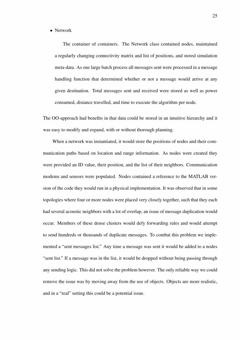
• Network
The container of containers. The Network class contained nodes, maintained
a regularly changing connectivity matrix and list of positions, and stored simulation
meta-data. As one large batch process all messages sent were processed in a message
handling function that determined whether or not a message would arrive at any
given destination. Total messages sent and received were stored as well as power
consumed, distance travelled, and time to execute the algorithm per node.
The OO-approach had benefits in that data could be stored in an intuitive hierarchy and it
was easy to modify and expand, with or without thorough planning.
When a network was instantiated, it would store the positions of nodes and their com-
munication paths based on location and range information. As nodes were created they
were provided an ID value, their position, and the list of their neighbors. Communication
modems and sensors were populated. Nodes contained a reference to the MATLAB ver-
sion of the code they would run in a physical implementation. It was observed that in some
topologies where four or more nodes were placed very closely together, such that they each
had several acoustic neighbors with a lot of overlap, an issue of message duplication would
occur. Members of these dense clusters would defy forwarding rules and would attempt
to send hundreds or thousands of duplicate messages. To combat this problem we imple-
mented a “sent messages list.” Any time a message was sent it would be added to a nodes
“sent list.” If a message was in the list, it would be dropped without being passing through
any sending logic. This did not solve the problem however. The only reliable way we could
remove the issue was by moving away from the use of objects. Objects are more realistic,
and in a “real” setting this could be a potential issue.
26
This work is abstract, not a low-level system that needs to precisely follow real-world
issues. It was not possible to reliably obtain data and ensure a fair comparison between
algorithms using this approach. Out of necessity the OO environment was abandoned.
3.1.2 Procedural Environment. The final version of the environment is procedu-
ral with data in correlation arrays. The strengths of the implementation are its simplicity,
ease of adding features, improved maintainability, and a gain in performance acquired by
reducing the number of references. A collection of scripts establish and run the system with
helper functions where non-damaging change simplifies calculations. We separate scripts
and functions into three categories as follows:
• Initializers
These are single purpose scripts. They initialize a data field (node positions, mes-
sage queues) and define a constants, such as radio range, that will be used throughout
the simulation.
• Modifiers
Generally implemented as functions, they make temporary partial-copies of ma-
trices and return the result. A prime example of this is the handling of messages
queues. There is a function called add2buffer that takes as parameters the message
queue, its read and write pointers, and the new message. Returned is the modified
queue and pointers. Modifiers are helper functions, and sometimes scripts, that ma-
nipulate storage structures rather than just using them.
• Run-Time
27
Running the simulation and the algorithmic-helpers. The process of generating
messages, determining how to respond, and constructing the path radio messages
will follow, are all run-time tasks. Along with the aptly named Sim Run script, are
the scripts for the routing algorithms.
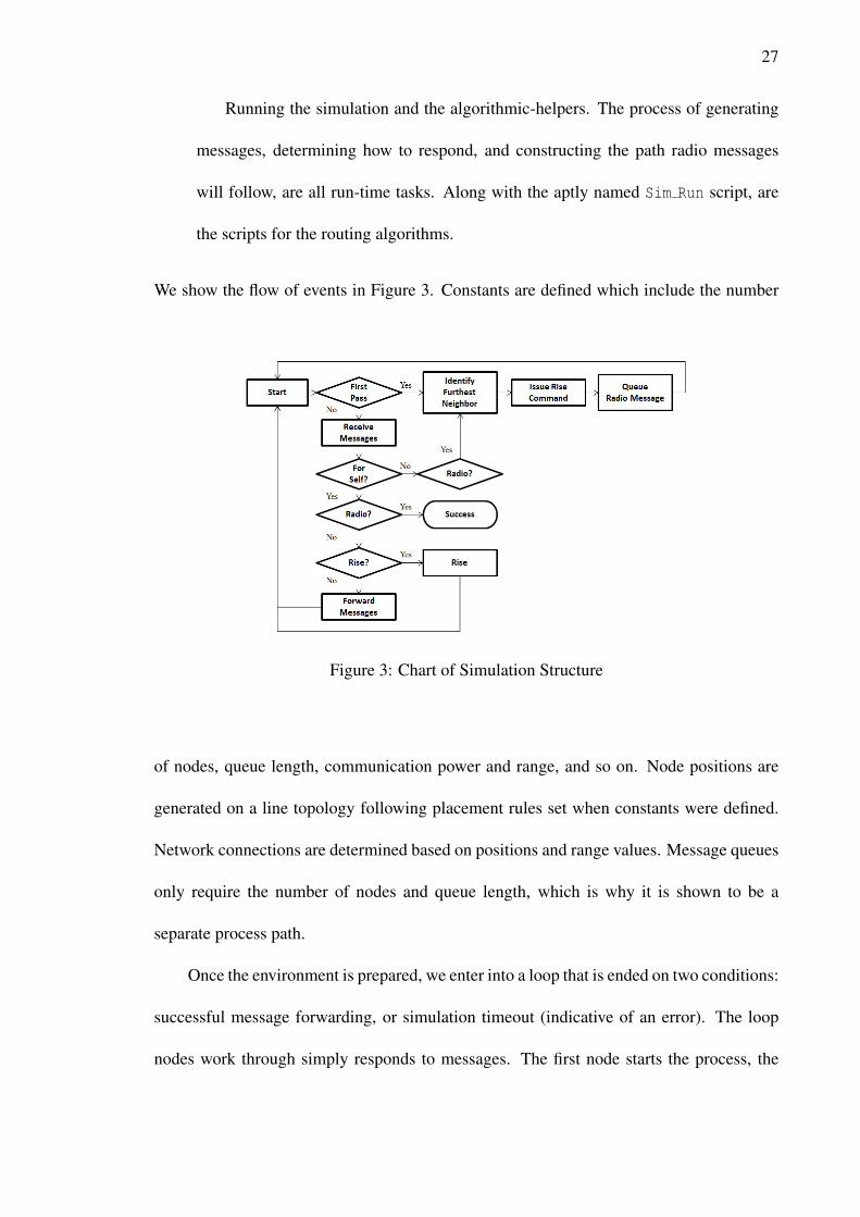
We show the flow of events in Figure 3. Constants are defined which include the number
Figure 3: Chart of Simulation Structure
of nodes, queue length, communication power and range, and so on. Node positions are
generated on a line topology following placement rules set when constants were defined.
Network connections are determined based on positions and range values. Message queues
only require the number of nodes and queue length, which is why it is shown to be a
separate process path.
Once the environment is prepared, we enter into a loop that is ended on two conditions:
successful message forwarding, or simulation timeout (indicative of an error). The loop
nodes work through simply responds to messages. The first node starts the process, the
28
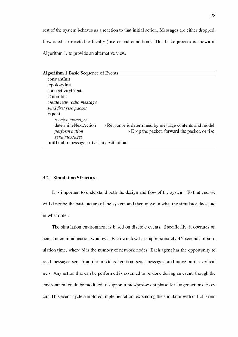
rest of the system behaves as a reaction to that initial action. Messages are either dropped,
forwarded, or reacted to locally (rise or end-condition). This basic process is shown in
Algorithm 1, to provide an alternative view.
Algorithm 1 Basic Sequence of EventsconstantInittopologyInitconnectivityCreateCommInitcreate new radio messagesend first rise packetrepeat
receive messagesdetermineNextAction . Response is determined by message contents and model.perform action . Drop the packet, forward the packet, or rise.send messages
until radio message arrives at destination
3.2 Simulation Structure
It is important to understand both the design and flow of the system. To that end we
will describe the basic nature of the system and then move to what the simulator does and
in what order.
The simulation environment is based on discrete events. Specifically, it operates on
acoustic-communication windows. Each window lasts approximately 4N seconds of sim-
ulation time, where N is the number of network nodes. Each agent has the opportunity to
read messages sent from the previous iteration, send messages, and move on the vertical
axis. Any action that can be performed is assumed to be done during an event, though the
environment could be modified to support a pre-/post-event phase for longer actions to oc-
cur. This event-cycle simplified implementation; expanding the simulator with out-of-event

29
processing would restore some realism to the system. Armed with this understanding of
what the simulator does, and the description is basic components, we move on to simulation
flow.
As shown in Algorithm 1, the simulator initializes the environment and launches a
run script. The result of the simulation is a collection of matrices that contain data on
position, messages sent and received, energy consumed, and time taken. The process of
running the simulation requires information on position, message queues, and communica-
tion modems (range, power). Initialization is separated across four files: constantInit,
topologyInit, connectivityCreate, and CommInit.
The script constantInit checks to see if required constants have been defined al-
ready, and sets them if they do not exist. These values include but are not limited to the
range and power of the radio and acoustic modems, the maximum length of a message
queue, the energy cost of different actions, and the number of nodes to generate. Topolo-
gies are either generated or imported using the topologyInit script. This script checks to
see if positions have been defined, and if not it generates a random line topology within de-
fined constraints. From the topology, connectivityCreate uses modem ranges to create
a connectivity matrix for each communication modem. The connectivity matrix is an NxN
logical matrix, where true represents a connection. CommInit creates message queues,
implemented as ring buffers, using the number of nodes and the queue length.
After initialization Sim Run uses constants defined in constantInit and the struc-
tures from the other initializers to determine the radio path, simulate the message-passing
process, and generally emulate idealized behavior of individual nodes.
30
3.3 Environment Performance Metrics
In this section we define how we measure environment performance. Aside from
whether the result is correct or not, we can determine performance by how much time is
required for networks of different size, and how much memory the system uses. Naturally,
when comparing implementations the better choice is the one that minimizes necessary
resources. If two have identical spatial requirements yet one is clearly faster, it is the
superior implementation, mutatis mutandi for fixed time and differing space. Following is
a description of how we measure time and memory requirements in MATLAB on Windows
and Linux platforms.
3.3.1 How Time is Measured. Built in to MATLAB are the functions tic and
toc. These respectively start a timer and calculate the approximate number of seconds that
have elapsed since the timer was started. This is the simplest way in which to monitor
the performance on a given system. It is platform independent, which makes it a natural
choice.
3.3.2 How Memory is Measured. MATLAB has two methods of reporting mem-
ory usage. One is a Windows-only command called memory, and the other is whos. The
former reports out byte-usage of the entire platform, and will provide information relating
to memory pages and other low level information. The latter iterates through all variables
in the current workspace and reports the number of bytes each item consumes. We use
whos for this project. Using memory or using an operating system tool such as top on
Linux provides information about the entire system. For a true comparison, we use whos,
as this will avoid any background tasks that MATLAB undertakes during simulation.
31
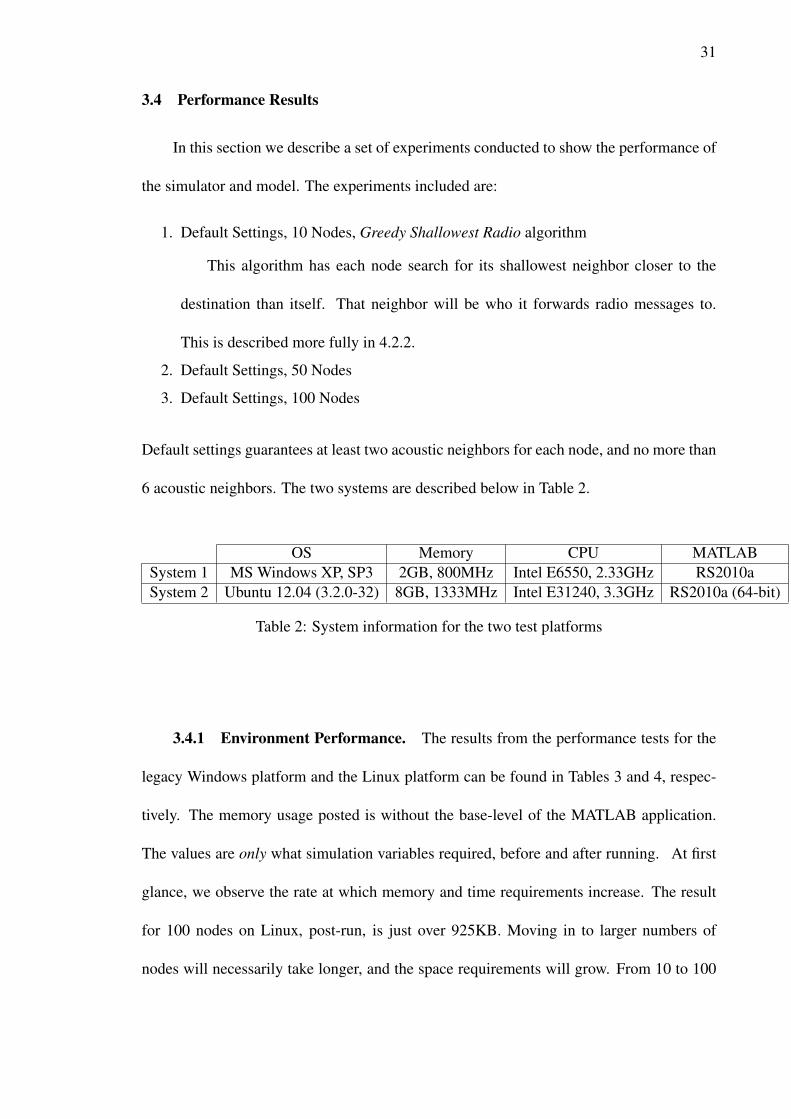
3.4 Performance Results
In this section we describe a set of experiments conducted to show the performance of
the simulator and model. The experiments included are:
1. Default Settings, 10 Nodes, Greedy Shallowest Radio algorithm
This algorithm has each node search for its shallowest neighbor closer to the
destination than itself. That neighbor will be who it forwards radio messages to.
This is described more fully in 4.2.2.
2. Default Settings, 50 Nodes
3. Default Settings, 100 Nodes
Default settings guarantees at least two acoustic neighbors for each node, and no more than
6 acoustic neighbors. The two systems are described below in Table 2.
OS Memory CPU MATLABSystem 1 MS Windows XP, SP3 2GB, 800MHz Intel E6550, 2.33GHz RS2010aSystem 2 Ubuntu 12.04 (3.2.0-32) 8GB, 1333MHz Intel E31240, 3.3GHz RS2010a (64-bit)
Table 2: System information for the two test platforms
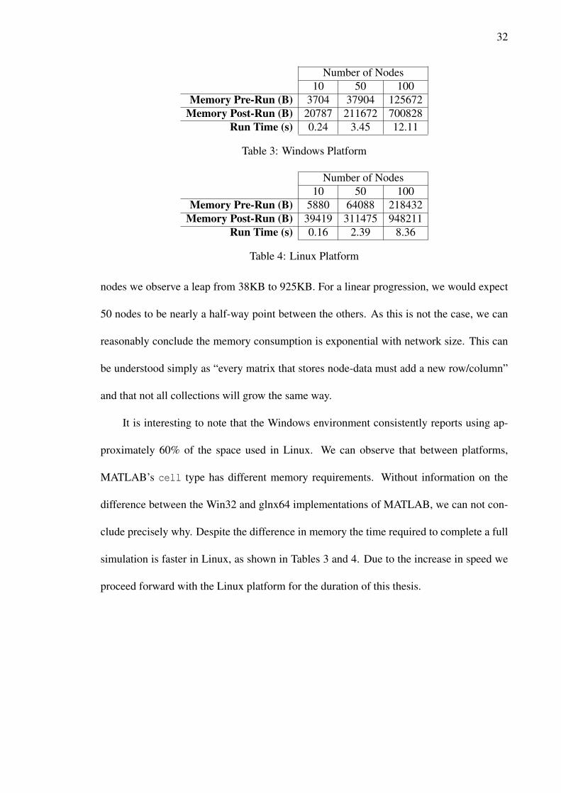
3.4.1 Environment Performance. The results from the performance tests for the
legacy Windows platform and the Linux platform can be found in Tables 3 and 4, respec-
tively. The memory usage posted is without the base-level of the MATLAB application.
The values are only what simulation variables required, before and after running. At first
glance, we observe the rate at which memory and time requirements increase. The result
for 100 nodes on Linux, post-run, is just over 925KB. Moving in to larger numbers of
nodes will necessarily take longer, and the space requirements will grow. From 10 to 100
32
Number of Nodes10 50 100
Memory Pre-Run (B) 3704 37904 125672Memory Post-Run (B) 20787 211672 700828
Run Time (s) 0.24 3.45 12.11
Table 3: Windows Platform
Number of Nodes10 50 100
Memory Pre-Run (B) 5880 64088 218432Memory Post-Run (B) 39419 311475 948211
Run Time (s) 0.16 2.39 8.36
Table 4: Linux Platform
nodes we observe a leap from 38KB to 925KB. For a linear progression, we would expect
50 nodes to be nearly a half-way point between the others. As this is not the case, we can
reasonably conclude the memory consumption is exponential with network size. This can
be understood simply as “every matrix that stores node-data must add a new row/column”
and that not all collections will grow the same way.
It is interesting to note that the Windows environment consistently reports using ap-
proximately 60% of the space used in Linux. We can observe that between platforms,
MATLAB’s cell type has different memory requirements. Without information on the
difference between the Win32 and glnx64 implementations of MATLAB, we can not con-
clude precisely why. Despite the difference in memory the time required to complete a full
simulation is faster in Linux, as shown in Tables 3 and 4. Due to the increase in speed we
proceed forward with the Linux platform for the duration of this thesis.
33
Chapter 4: Algorithms Implemented
In this chapter we discuss the algorithms we implemented. There are a total of eight
different algorithms separated into two categories. The categories are “acoustic-centric”
and “radio-centric” algorithms. An algorithm is considered acoustic-centric if routing de-
cisions are made from information on acoustic neighbors. So, naturally, a radio-centric
method is one that makes decisions based off of radio neighbors.
All of these algorithms rely on the connectivity matrix defined in 3.2. In short, a log-
ical matrix where true represents a connection, and the connections are determined by the
distance between nodes and the range of the active modem. Further, all of the algorithms
assume radio range is greater than or equal to acoustic range. This is not a requirement of
the environment, it is only a detail of how they were implemented. This was done to sim-
plify implementation, and with relatively minor changes each algorithm could be modified
to be range-agnostic. The final requirement imposed, that is necessary for a successful sim-
ulation, is that each node have at least one acoustic neighbor. This automatically guarantees
a minimum of one radio neighbor because if two nodes are within acoustic range, they are
guaranteed to be within radio range. For any algorithm, the general sequence of events
is: receive a radio message, identify the next-hop in the path, issue a rise command, and
forward the radio message after a short delay. An example of this can be seen in Algorithm
1, which shows the generic process from start to finish.
The rest of this chapter is separated as discussions of acoustic algorithms and radio
34
algorithms respectively. The algorithms are discussed and sample data for each is provided.
4.1 Acoustic-Centric Algorithms
There are two acoustic-centric algorithms. A furthest-neighbor approach and a shallowest-
neighbor approach. These are called Greedy Furthest Acoustic and Greedy Shallowest
Acoustic, respectively.
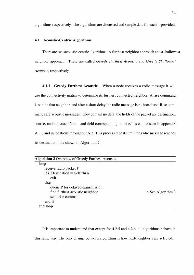
4.1.1 Greedy Furthest Acoustic. When a node receives a radio message it will
use the connectivity matrix to determine its furthest connected neighbor. A rise command
is sent to that neighbor, and after a short delay the radio message is re-broadcast. Rise com-
mands are acoustic messages. They contain no data; the fields of the packet are destination,
source, and a protocol/command field corresponding to “rise,” as can be seen in appendix
A.3.3 and in locations throughout A.2. This process repeats until the radio message reaches
its destination, like shown in Algorithm 2.
Algorithm 2 Overview of Greedy Furthest Acousticloop
receive radio packet Pif P.Destination ≡ Self then
exitelse
queue P for delayed-transmissionfind furthest acoustic neighbor . See Algorithm 3send rise command
end ifend loop
It is important to understand that except for 4.2.5 and 4.2.6, all algorithms behave in
this same way. The only change between algorithms is how next-neighbor’s are selected.
35
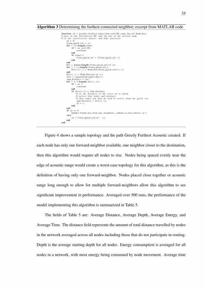
Algorithm 3 Determining the furthest connected neighbor; excerpt from MATLAB codef u n c t i o n i d = g r e e d y f a r t h e s t a l g o r i t h m ( s e l f I D , conn , d s t i d , Node Pos )
% pass i n t h e d e s t i n a t i o n ID , and t h e row o f t h e p r e s e n t node% i n t h e c o n n e c t i v i t y ma t r i x , and node p o s i t i o n s
i d = 0 ;C o n n q u i c k r e f = [ ] ;f o r i =1 : l e n g t h ( conn )
i f i == s e l f I D ;c o n t i n u e
endi f conn ( i )
C o n n q u i c k r e f = [ C o n n q u i c k r e f i ] ;end
endPos = z e r o s ( l e n g t h ( C o n n q u i c k r e f ) + 1 , 1 ) ;f o r i = 1 : ( l e n g t h ( C o n n q u i c k r e f ) )
Pos ( i + 1 , : ) = Node Pos ( C o n n q u i c k r e f ( i ) , 1 ) ;endPos ( 1 , : ) = Node Pos ( d s t i d , 1 ) ;d i s t = s q u a r e f o r m ( p d i s t ( Pos ) ) ;t m p d i s t a n c e = i n f ;f o r i = 1 : l e n g t h ( d i s t ( : , 1 ) )
i f i == 1c o n t i n u e
endi f d i s t ( i , 1 ) < t m p d i s t a n c e
% i f t h e d i s t a n c e i s t h e l e a s t we ’ ve found% s e l e c t t h a t i n d e x and d i s t a n c e% t h a t i n d e x can t h e n be used t o s e l e c t from t h e q u i c k r e f .t m p d i s t a n c e = d i s t ( i , 1 ) ;i d = i ;
endendi f i d == 0
error ( ’ Could n o t f i n d any n e i g h b o r s , which i s n o t l i k e l y . \ n ’ )e l s e
i d = C o n n q u i c k r e f ( i d − 1 ) ;end
end
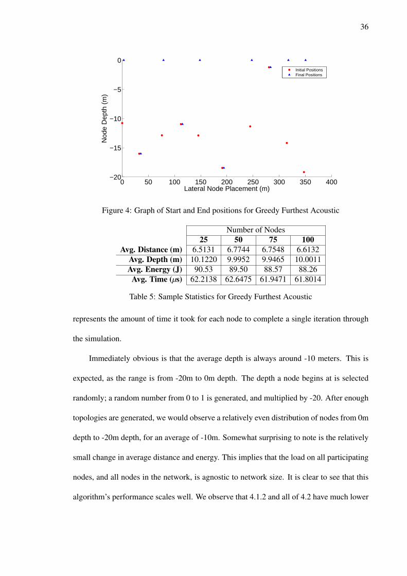
Figure 4 shows a sample topology and the path Greedy Furthest Acoustic created. If
each node has only one forward-neighbor available, one neighbor closer to the destination,
then this algorithm would require all nodes to rise. Nodes being spaced evenly near the
edge of acoustic range would create a worst-case topology for this algorithm, as this is the
definition of having only one forward-neighbor. Nodes placed close together or acoustic
range long enough to allow for multiple forward-neighbors allow this algorithm to see
significant improvement in performance. Averaged over 500 runs, the performance of the
model implementing this algorithm is summarized in Table 5.
The fields of Table 5 are: Average Distance, Average Depth, Average Energy, and
Average Time. The distance field represents the amount of total distance travelled by nodes
in the network averaged across all nodes including those that do not participate in routing.
Depth is the average starting depth for all nodes. Energy consumption is averaged for all
nodes in a network, with most energy being consumed by node movement. Average time
36
0 50 100 150 200 250 300 350 400−20
−15
−10
−5
0
Lateral Node Placement (m)
Nod
e D
epth
(m
)
Initial PositionsFinal Positions
Figure 4: Graph of Start and End positions for Greedy Furthest Acoustic
Number of Nodes25 50 75 100
Avg. Distance (m) 6.5131 6.7744 6.7548 6.6132Avg. Depth (m) 10.1220 9.9952 9.9465 10.0011Avg. Energy (J) 90.53 89.50 88.57 88.26
Avg. Time (µs) 62.2138 62.6475 61.9471 61.8014
Table 5: Sample Statistics for Greedy Furthest Acoustic
represents the amount of time it took for each node to complete a single iteration through
the simulation.
Immediately obvious is that the average depth is always around -10 meters. This is
expected, as the range is from -20m to 0m depth. The depth a node begins at is selected
randomly; a random number from 0 to 1 is generated, and multiplied by -20. After enough
topologies are generated, we would observe a relatively even distribution of nodes from 0m
depth to -20m depth, for an average of -10m. Somewhat surprising to note is the relatively
small change in average distance and energy. This implies that the load on all participating
nodes, and all nodes in the network, is agnostic to network size. It is clear to see that this
algorithm’s performance scales well. We observe that 4.1.2 and all of 4.2 have much lower
37
energy requirements than Greedy Furthest Acoustic.
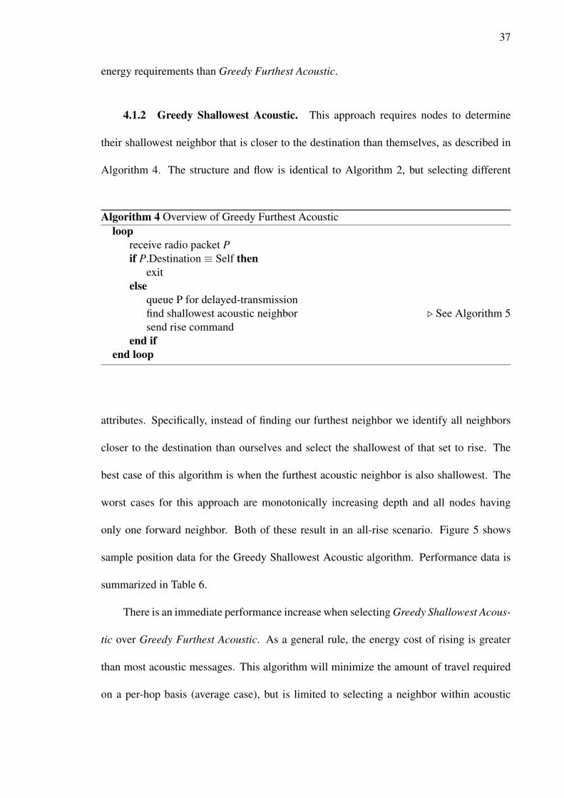
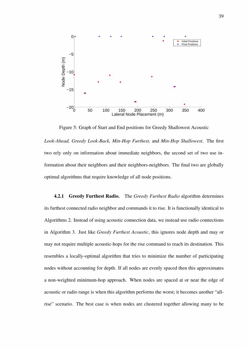
4.1.2 Greedy Shallowest Acoustic. This approach requires nodes to determine
their shallowest neighbor that is closer to the destination than themselves, as described in
Algorithm 4. The structure and flow is identical to Algorithm 2, but selecting different
Algorithm 4 Overview of Greedy Furthest Acousticloop
receive radio packet Pif P.Destination ≡ Self then
exitelse
queue P for delayed-transmissionfind shallowest acoustic neighbor . See Algorithm 5send rise command
end ifend loop
attributes. Specifically, instead of finding our furthest neighbor we identify all neighbors
closer to the destination than ourselves and select the shallowest of that set to rise. The
best case of this algorithm is when the furthest acoustic neighbor is also shallowest. The
worst cases for this approach are monotonically increasing depth and all nodes having
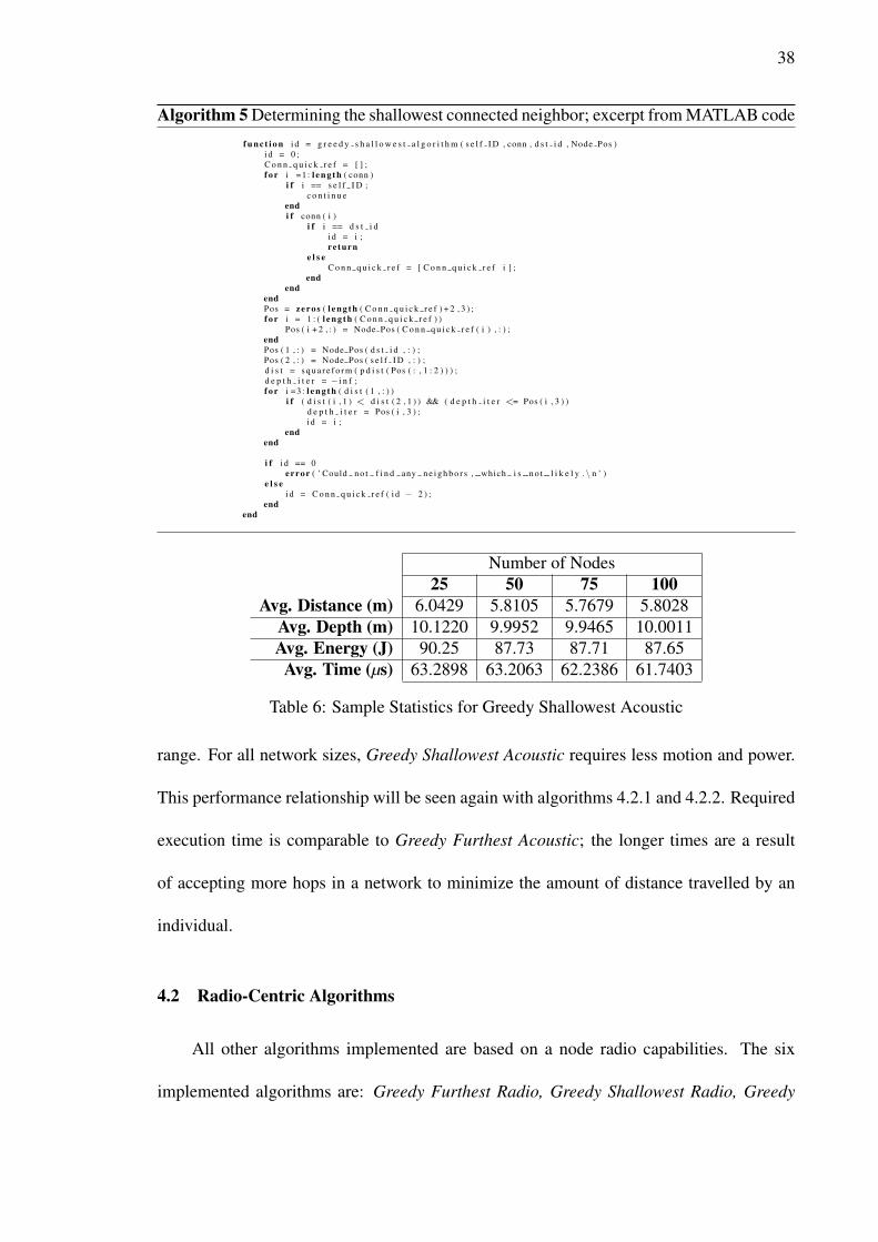
only one forward neighbor. Both of these result in an all-rise scenario. Figure 5 shows
sample position data for the Greedy Shallowest Acoustic algorithm. Performance data is
summarized in Table 6.
There is an immediate performance increase when selecting Greedy Shallowest Acous-
tic over Greedy Furthest Acoustic. As a general rule, the energy cost of rising is greater
than most acoustic messages. This algorithm will minimize the amount of travel required
on a per-hop basis (average case), but is limited to selecting a neighbor within acoustic
38
Algorithm 5 Determining the shallowest connected neighbor; excerpt from MATLAB codef u n c t i o n i d = g r e e d y s h a l l o w e s t a l g o r i t h m ( s e l f I D , conn , d s t i d , Node Pos )
i d = 0 ;C o n n q u i c k r e f = [ ] ;f o r i =1 : l e n g t h ( conn )
i f i == s e l f I D ;c o n t i n u e
endi f conn ( i )
i f i == d s t i di d = i ;re turn
e l s eC o n n q u i c k r e f = [ C o n n q u i c k r e f i ] ;
endend
endPos = z e r o s ( l e n g t h ( C o n n q u i c k r e f ) + 2 , 3 ) ;f o r i = 1 : ( l e n g t h ( C o n n q u i c k r e f ) )
Pos ( i + 2 , : ) = Node Pos ( C o n n q u i c k r e f ( i ) , : ) ;endPos ( 1 , : ) = Node Pos ( d s t i d , : ) ;Pos ( 2 , : ) = Node Pos ( s e l f I D , : ) ;d i s t = s q u a r e f o r m ( p d i s t ( Pos ( : , 1 : 2 ) ) ) ;d e p t h i t e r = − i n f ;f o r i =3 : l e n g t h ( d i s t ( 1 , : ) )
i f ( d i s t ( i , 1 ) < d i s t ( 2 , 1 ) ) && ( d e p t h i t e r <= Pos ( i , 3 ) )d e p t h i t e r = Pos ( i , 3 ) ;i d = i ;
endend
i f i d == 0error ( ’ Could n o t f i n d any n e i g h b o r s , which i s n o t l i k e l y . \ n ’ )
e l s ei d = C o n n q u i c k r e f ( i d − 2 ) ;
endend
Number of Nodes25 50 75 100
Avg. Distance (m) 6.0429 5.8105 5.7679 5.8028Avg. Depth (m) 10.1220 9.9952 9.9465 10.0011Avg. Energy (J) 90.25 87.73 87.71 87.65
Avg. Time (µs) 63.2898 63.2063 62.2386 61.7403
Table 6: Sample Statistics for Greedy Shallowest Acoustic
range. For all network sizes, Greedy Shallowest Acoustic requires less motion and power.
This performance relationship will be seen again with algorithms 4.2.1 and 4.2.2. Required
execution time is comparable to Greedy Furthest Acoustic; the longer times are a result
of accepting more hops in a network to minimize the amount of distance travelled by an
individual.
4.2 Radio-Centric Algorithms
All other algorithms implemented are based on a node radio capabilities. The six
implemented algorithms are: Greedy Furthest Radio, Greedy Shallowest Radio, Greedy
39
0 50 100 150 200 250 300 350 400−20
−15
−10
−5
0
Lateral Node Placement (m)
Nod
e D
epth
(m
)
Initial PositionsFinal Positions
Figure 5: Graph of Start and End positions for Greedy Shallowest Acoustic
Look-Ahead, Greedy Look-Back, Min-Hop Furthest, and Min-Hop Shallowest. The first
two rely only on information about immediate neighbors, the second set of two use in-
formation about their neighbors and their neighbors-neighbors. The final two are globally
optimal algorithms that require knowledge of all node positions.
4.2.1 Greedy Furthest Radio. The Greedy Furthest Radio algorithm determines
its furthest connected radio neighbor and commands it to rise. It is functionally identical to
Algorithms 2. Instead of using acoustic connection data, we instead use radio connections
in Algorithm 3. Just like Greedy Furthest Acoustic, this ignores node depth and may or
may not require multiple acoustic-hops for the rise command to reach its destination. This
resembles a locally-optimal algorithm that tries to minimize the number of participating
nodes without accounting for depth. If all nodes are evenly spaced then this approximates
a non-weighted minimum-hop approach. When nodes are spaced at or near the edge of
acoustic or radio range is when this algorithm performs the worst; it becomes another “all-
rise” scenario. The best case is when nodes are clustered together allowing many to be
40
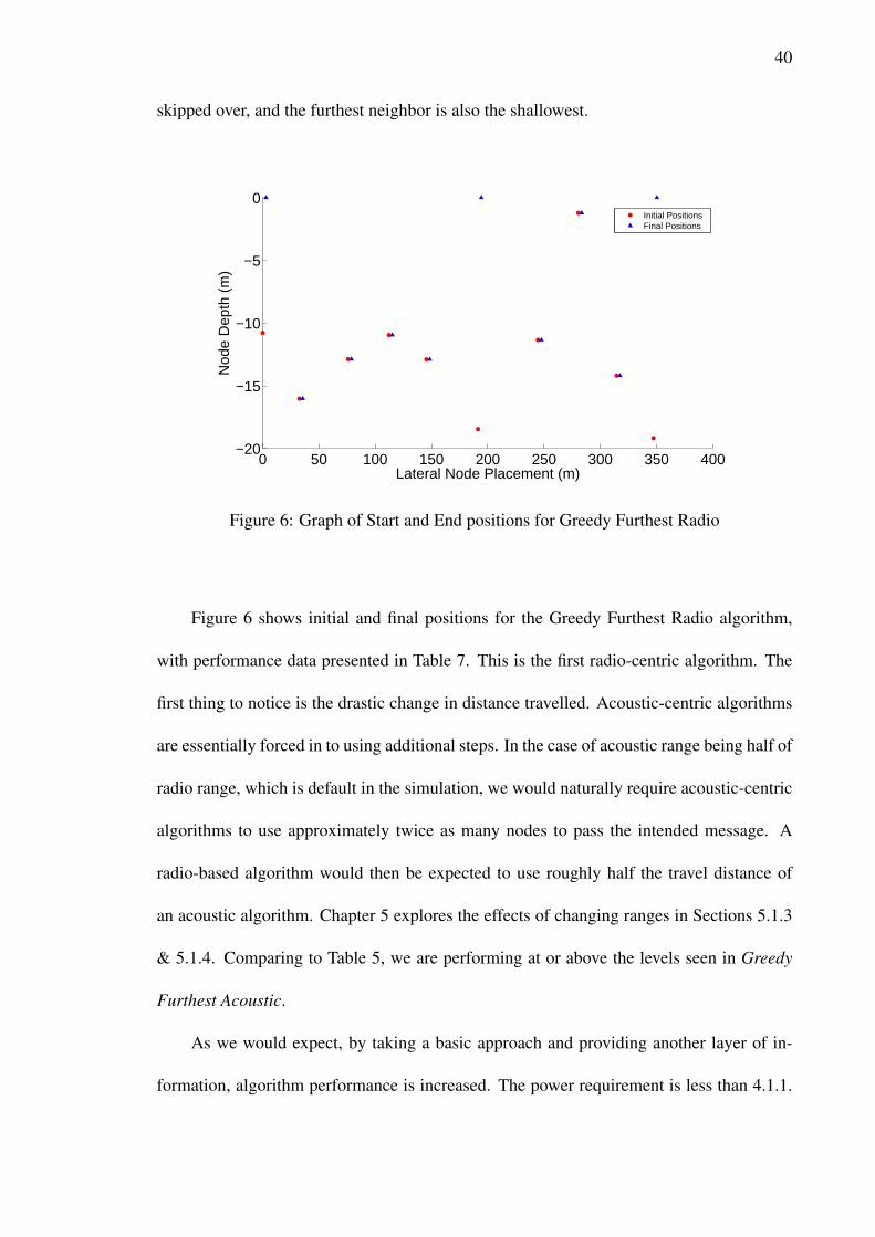
skipped over, and the furthest neighbor is also the shallowest.
0 50 100 150 200 250 300 350 400−20
−15
−10
−5
0
Lateral Node Placement (m)
Nod
e D
epth
(m
)
Initial PositionsFinal Positions
Figure 6: Graph of Start and End positions for Greedy Furthest Radio
Figure 6 shows initial and final positions for the Greedy Furthest Radio algorithm,
with performance data presented in Table 7. This is the first radio-centric algorithm. The
first thing to notice is the drastic change in distance travelled. Acoustic-centric algorithms
are essentially forced in to using additional steps. In the case of acoustic range being half of
radio range, which is default in the simulation, we would naturally require acoustic-centric
algorithms to use approximately twice as many nodes to pass the intended message. A
radio-based algorithm would then be expected to use roughly half the travel distance of
an acoustic algorithm. Chapter 5 explores the effects of changing ranges in Sections 5.1.3
& 5.1.4. Comparing to Table 5, we are performing at or above the levels seen in Greedy
Furthest Acoustic.
As we would expect, by taking a basic approach and providing another layer of in-
formation, algorithm performance is increased. The power requirement is less than 4.1.1.
41
This is solely due to the decreased number of nodes participating in routing. Fewer nodes
are required to participate, so less power is used in moving.
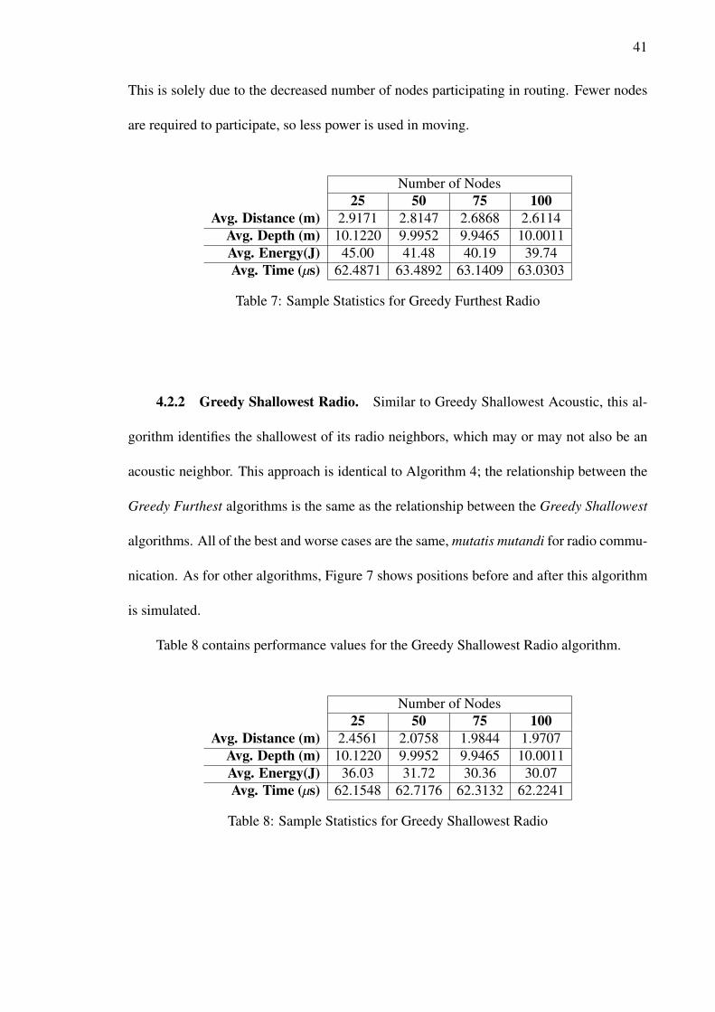
Number of Nodes25 50 75 100
Avg. Distance (m) 2.9171 2.8147 2.6868 2.6114Avg. Depth (m) 10.1220 9.9952 9.9465 10.0011Avg. Energy(J) 45.00 41.48 40.19 39.74Avg. Time (µs) 62.4871 63.4892 63.1409 63.0303
Table 7: Sample Statistics for Greedy Furthest Radio
4.2.2 Greedy Shallowest Radio. Similar to Greedy Shallowest Acoustic, this al-
gorithm identifies the shallowest of its radio neighbors, which may or may not also be an
acoustic neighbor. This approach is identical to Algorithm 4; the relationship between the
Greedy Furthest algorithms is the same as the relationship between the Greedy Shallowest
algorithms. All of the best and worse cases are the same, mutatis mutandi for radio commu-
nication. As for other algorithms, Figure 7 shows positions before and after this algorithm
is simulated.
Table 8 contains performance values for the Greedy Shallowest Radio algorithm.
Number of Nodes25 50 75 100
Avg. Distance (m) 2.4561 2.0758 1.9844 1.9707Avg. Depth (m) 10.1220 9.9952 9.9465 10.0011Avg. Energy(J) 36.03 31.72 30.36 30.07Avg. Time (µs) 62.1548 62.7176 62.3132 62.2241
Table 8: Sample Statistics for Greedy Shallowest Radio

42
0 50 100 150 200 250 300 350 400−20
−15
−10
−5
0
Lateral Node Placement (m)
Nod
e D
epth
(m
)
Initial PositionsFinal Positions
Figure 7: Graph of Start and End positions for Greedy Shallowest Radio
In comparison to 4.1.2 it is again made clear that with the increase in information,
performance is increased. Just as when 4.2.1 was found to perform at over twice the levels
of 4.1.1, so to does Greedy Shallowest Radio perform over twice as well as 4.1.2. Further-
more, as stated previously, Greedy Shallowest Radio out-performs Greedy Furthest Radio.
The relationship follows exactly the same as for their acoustic counterparts.
4.2.3 Greedy Look-Ahead. This is the first algorithm that requires the addition
of neighbor’s-neighbors positions. Greedy Look-Ahead uses connection information span-
ning out to the furthest radio neighbor’s furthest neighbor, and is described in Algorithm 7.
It then calculates the optimal next step using Dijkstra’s algorithm with link-costs being
weighted by node depth. The only requirements placed on the system are: no-backwards
traversals (messages always advance) and the path chosen must have a length greater than
two (not including the sender). The path length requirement is a safe-guard against be-
coming a purely shallowest-neighbor approach. The minimum weight path is selected, and
43
Algorithm 6 Overview of Greedy Look-Aheadloop
receive radio packet Pif P.Destination ≡ Self then
exitelse
queue P for delayed-transmissionConnections← connection data inlcuding furthest neighbor’s furthest neighborpaths← dijkstra(Positions, Connections, Self) . See Algorithm 7delete all paths from paths of length less than 2select lowest-cost pathsend rise command to next-hop
end ifend loop
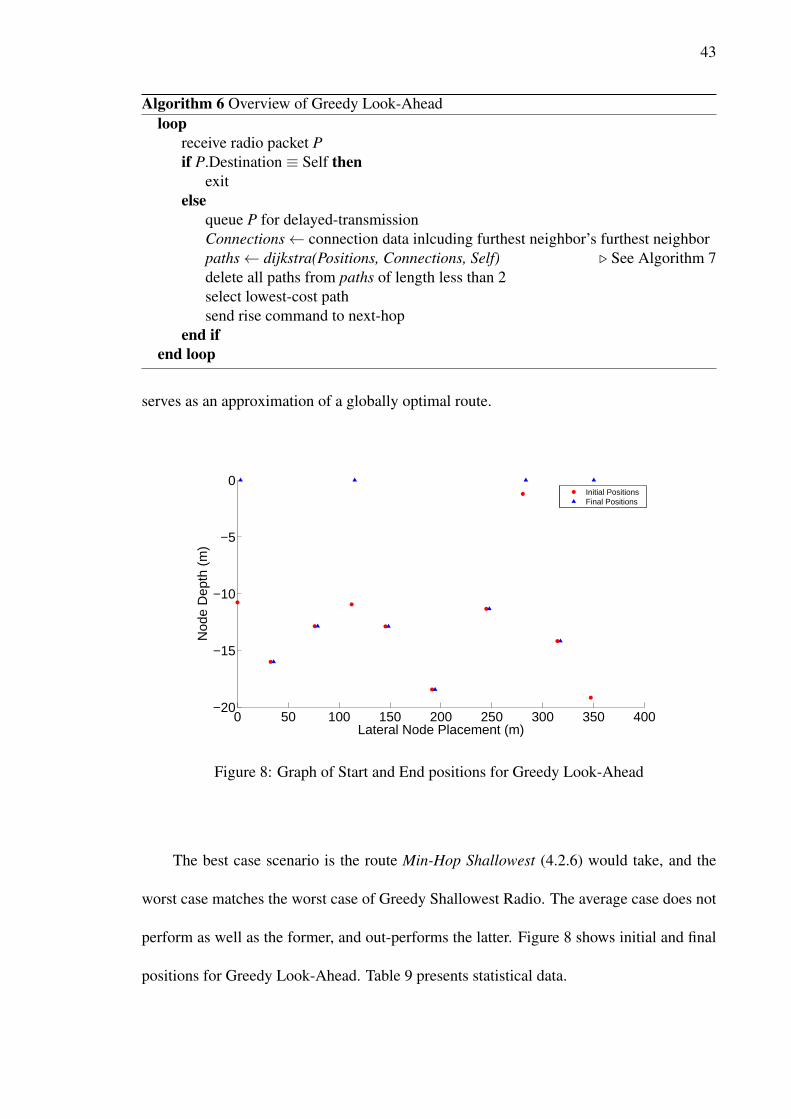
serves as an approximation of a globally optimal route.
0 50 100 150 200 250 300 350 400−20
−15
−10
−5
0
Lateral Node Placement (m)
Nod
e D
epth
(m
)
Initial PositionsFinal Positions
Figure 8: Graph of Start and End positions for Greedy Look-Ahead
The best case scenario is the route Min-Hop Shallowest (4.2.6) would take, and the
worst case matches the worst case of Greedy Shallowest Radio. The average case does not
perform as well as the former, and out-performs the latter. Figure 8 shows initial and final
positions for Greedy Look-Ahead. Table 9 presents statistical data.
44
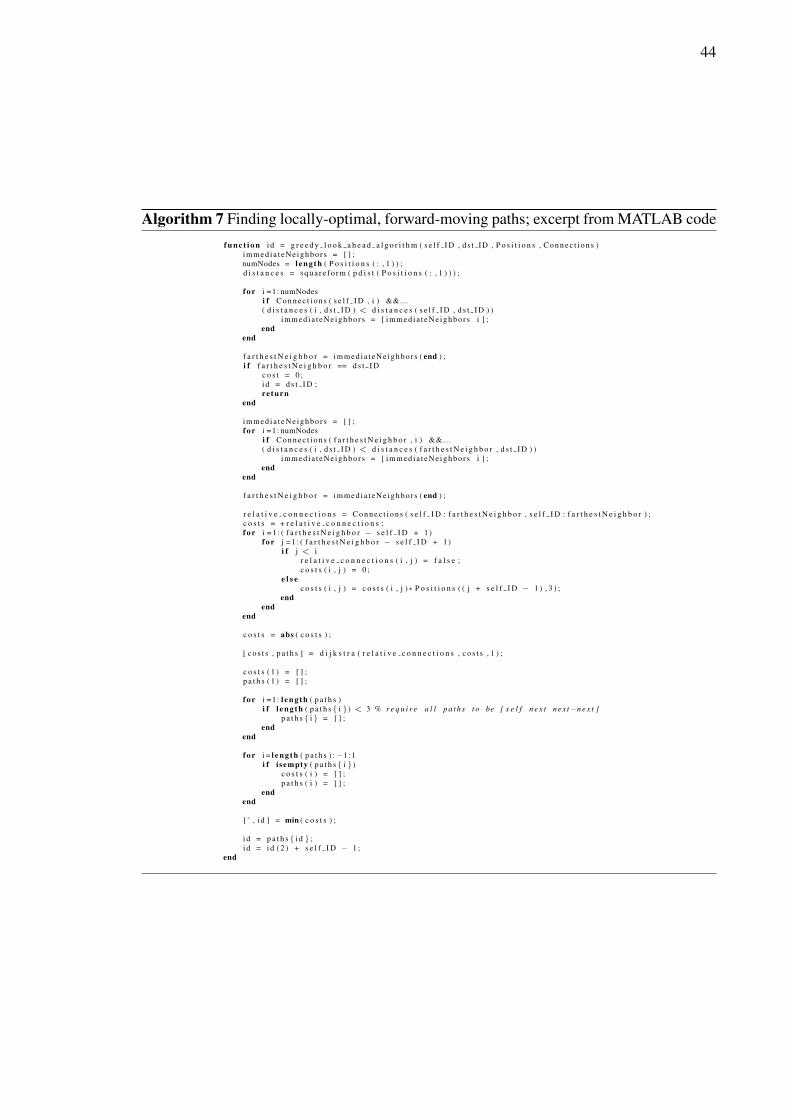
Algorithm 7 Finding locally-optimal, forward-moving paths; excerpt from MATLAB codef u n c t i o n i d = g r e e d y l o o k a h e a d a l g o r i t h m ( s e l f I D , d s t I D , P o s i t i o n s , C o n n e c t i o n s )
i m m e d i a t e N e i g h b o r s = [ ] ;numNodes = l e n g t h ( P o s i t i o n s ( : , 1 ) ) ;d i s t a n c e s = s q u a r e f o r m ( p d i s t ( P o s i t i o n s ( : , 1 ) ) ) ;
f o r i =1 : numNodesi f C o n n e c t i o n s ( s e l f I D , i ) &&. . .( d i s t a n c e s ( i , d s t I D ) < d i s t a n c e s ( s e l f I D , d s t I D ) )
i m m e d i a t e N e i g h b o r s = [ i m m e d i a t e N e i g h b o r s i ] ;end
end
f a r t h e s t N e i g h b o r = i m m e d i a t e N e i g h b o r s ( end ) ;i f f a r t h e s t N e i g h b o r == d s t I D
c o s t = 0 ;i d = d s t I D ;re turn
end
i m m e d i a t e N e i g h b o r s = [ ] ;f o r i =1 : numNodes
i f C o n n e c t i o n s ( f a r t h e s t N e i g h b o r , i ) &&. . .( d i s t a n c e s ( i , d s t I D ) < d i s t a n c e s ( f a r t h e s t N e i g h b o r , d s t I D ) )
i m m e d i a t e N e i g h b o r s = [ i m m e d i a t e N e i g h b o r s i ] ;end
end
f a r t h e s t N e i g h b o r = i m m e d i a t e N e i g h b o r s ( end ) ;
r e l a t i v e c o n n e c t i o n s = C o n n e c t i o n s ( s e l f I D : f a r t h e s t N e i g h b o r , s e l f I D : f a r t h e s t N e i g h b o r ) ;c o s t s = + r e l a t i v e c o n n e c t i o n s ;f o r i = 1 : ( f a r t h e s t N e i g h b o r − s e l f I D + 1)
f o r j = 1 : ( f a r t h e s t N e i g h b o r − s e l f I D + 1)i f j < i
r e l a t i v e c o n n e c t i o n s ( i , j ) = f a l s e ;c o s t s ( i , j ) = 0 ;
e l s ec o s t s ( i , j ) = c o s t s ( i , j )∗ P o s i t i o n s ( ( j + s e l f I D − 1 ) , 3 ) ;
endend
end
c o s t s = abs ( c o s t s ) ;
[ c o s t s , p a t h s ] = d i j k s t r a ( r e l a t i v e c o n n e c t i o n s , c o s t s , 1 ) ;
c o s t s ( 1 ) = [ ] ;p a t h s ( 1 ) = [ ] ;
f o r i =1 : l e n g t h ( p a t h s )i f l e n g t h ( p a t h s { i } ) < 3 % r e q u i r e a l l p a t h s t o be [ s e l f n e x t nex t−n e x t ]
p a t h s { i } = [ ] ;end
end
f o r i = l e n g t h ( p a t h s ) : −1 :1i f i sempty ( p a t h s { i } )
c o s t s ( i ) = [ ] ;p a t h s ( i ) = [ ] ;
endend
[ ˜ , i d ] = min ( c o s t s ) ;
i d = p a t h s { i d } ;i d = i d ( 2 ) + s e l f I D − 1 ;
end
45
Number of Nodes25 50 75 100
Avg. Distance (m) 2.2097 1.8510 1.7401 1.6957Avg. Depth (m) 10.1220 9.9952 9.9465 10.0011Avg. Energy(J) 32.57 27.86 26.27 25.97Avg. Time (µs) 79.3019 74.5612 68.6739 63.0941
Table 9: Sample Statistics for Greedy Look-Ahead
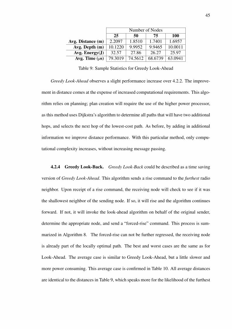
Greedy Look-Ahead observes a slight performance increase over 4.2.2. The improve-
ment in distance comes at the expense of increased computational requirements. This algo-
rithm relies on planning; plan creation will require the use of the higher power processor,
as this method uses Dijkstra’s algorithm to determine all paths that will have two additional
hops, and selects the next hop of the lowest-cost path. As before, by adding in additional
information we improve distance performance. With this particular method, only compu-
tational complexity increases, without increasing message passing.
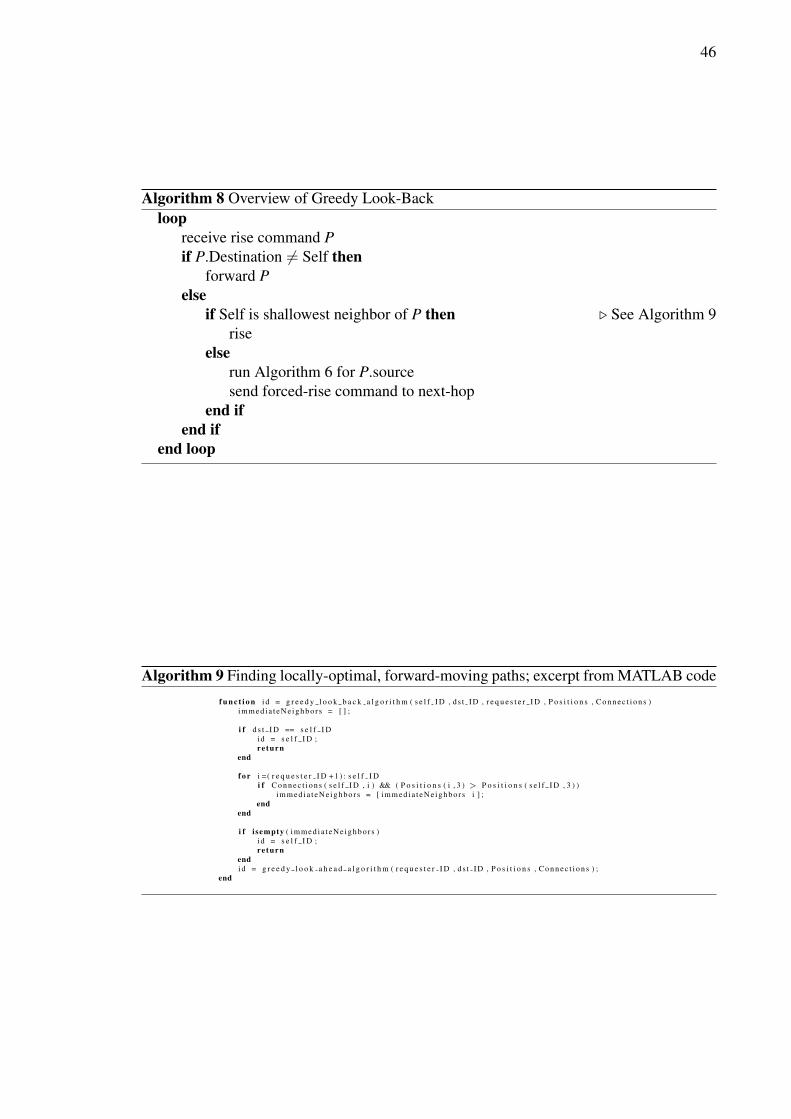
4.2.4 Greedy Look-Back. Greedy Look-Back could be described as a time saving
version of Greedy Look-Ahead. This algorithm sends a rise command to the furthest radio
neighbor. Upon receipt of a rise command, the receiving node will check to see if it was
the shallowest neighbor of the sending node. If so, it will rise and the algorithm continues
forward. If not, it will invoke the look-ahead algorithm on behalf of the original sender,
determine the appropriate node, and send a “forced-rise” command. This process is sum-
marized in Algorithm 8. The forced-rise can not be further regressed, the receiving node
is already part of the locally optimal path. The best and worst cases are the same as for
Look-Ahead. The average case is similar to Greedy Look-Ahead, but a little slower and
more power consuming. This average case is confirmed in Table 10. All average distances
are identical to the distances in Table 9, which speaks more for the likelihood of the furthest
46
Algorithm 8 Overview of Greedy Look-Backloop
receive rise command Pif P.Destination 6= Self then
forward Pelse
if Self is shallowest neighbor of P then . See Algorithm 9rise
elserun Algorithm 6 for P.sourcesend forced-rise command to next-hop
end ifend if
end loop
Algorithm 9 Finding locally-optimal, forward-moving paths; excerpt from MATLAB codef u n c t i o n i d = g r e e d y l o o k b a c k a l g o r i t h m ( s e l f I D , d s t I D , r e q u e s t e r I D , P o s i t i o n s , C o n n e c t i o n s )
i m m e d i a t e N e i g h b o r s = [ ] ;
i f d s t I D == s e l f I Di d = s e l f I D ;re turn
end
f o r i =( r e q u e s t e r I D + 1 ) : s e l f I Di f C o n n e c t i o n s ( s e l f I D , i ) && ( P o s i t i o n s ( i , 3 ) > P o s i t i o n s ( s e l f I D , 3 ) )
i m m e d i a t e N e i g h b o r s = [ i m m e d i a t e N e i g h b o r s i ] ;end
end
i f i sempty ( i m m e d i a t e N e i g h b o r s )i d = s e l f I D ;re turn
endi d = g r e e d y l o o k a h e a d a l g o r i t h m ( r e q u e s t e r I D , d s t I D , P o s i t i o n s , C o n n e c t i o n s ) ;
end
47
0 50 100 150 200 250 300 350 400−20
−15
−10
−5
0
Lateral Node Placement (m)
Nod
e D
epth
(m
)
Initial PositionsFinal Positions
Figure 9: Graph of Start and End positions for Greedy Look-Back
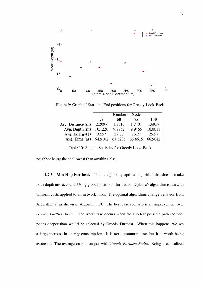
Number of Nodes25 50 75 100
Avg. Distance (m) 2.2097 1.8510 1.7401 1.6957Avg. Depth (m) 10.1220 9.9952 9.9465 10.0011Avg. Energy(J) 32.57 27.86 26.27 25.97Avg. Time (µs) 64.9102 67.6236 66.8615 66.5082
Table 10: Sample Statistics for Greedy Look-Back
neighbor being the shallowest than anything else.
4.2.5 Min-Hop Furthest. This is a globally optimal algorithm that does not take
node depth into account. Using global position information, Dijkstra’s algorithm is run with
uniform costs applied to all network links. The optimal algorithms change behavior from
Algorithm 2, as shown in Algorithm 10. The best case scenario is an improvement over
Greedy Furthest Radio. The worst case occurs when the shortest possible path includes
nodes deeper than would be selected by Greedy Furthest. When this happens, we see
a large increase in energy consumption. It is not a common case, but it is worth being
aware of. The average case is on par with Greedy Furthest Radio. Being a centralized
48
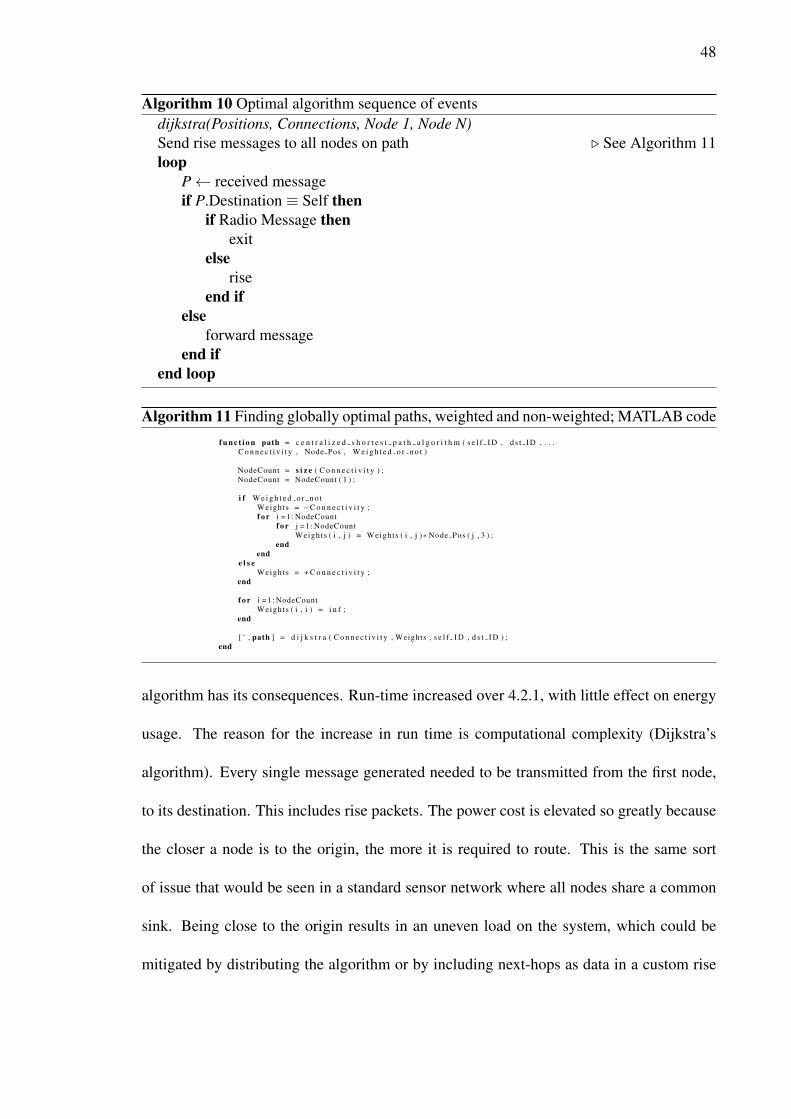
Algorithm 10 Optimal algorithm sequence of eventsdijkstra(Positions, Connections, Node 1, Node N)Send rise messages to all nodes on path . See Algorithm 11loop
P← received messageif P.Destination ≡ Self then
if Radio Message thenexit
elserise
end ifelse
forward messageend if
end loop
Algorithm 11 Finding globally optimal paths, weighted and non-weighted; MATLAB codef u n c t i o n path = c e n t r a l i z e d s h o r t e s t p a t h a l g o r i t h m ( s e l f I D , d s t I D , . . .
C o n n e c t i v i t y , Node Pos , W e i g h t e d o r n o t )
NodeCount = s i z e ( C o n n e c t i v i t y ) ;NodeCount = NodeCount ( 1 ) ;
i f W e i g h t e d o r n o tWeights = −C o n n e c t i v i t y ;f o r i =1 : NodeCount
f o r j =1 : NodeCountWeights ( i , j ) = Weights ( i , j )∗Node Pos ( j , 3 ) ;
endend
e l s eWeights = + C o n n e c t i v i t y ;
end
f o r i =1 : NodeCountWeights ( i , i ) = i n f ;
end
[ ˜ , path ] = d i j k s t r a ( C o n n e c t i v i t y , Weights , s e l f I D , d s t I D ) ;end
algorithm has its consequences. Run-time increased over 4.2.1, with little effect on energy
usage. The reason for the increase in run time is computational complexity (Dijkstra’s
algorithm). Every single message generated needed to be transmitted from the first node,
to its destination. This includes rise packets. The power cost is elevated so greatly because
the closer a node is to the origin, the more it is required to route. This is the same sort
of issue that would be seen in a standard sensor network where all nodes share a common
sink. Being close to the origin results in an uneven load on the system, which could be
mitigated by distributing the algorithm or by including next-hops as data in a custom rise

49
0 50 100 150 200 250 300 350 400−20
−15
−10
−5
0
Lateral Node Placement (m)
Nod
e D
epth
(m
)
Initial PositionsFinal Positions
Figure 10: Graph of Start and End positions for Min-Hop Furthest
Number of Nodes25 50 75 100
Avg. Distance (m) 3.0701 2.7676 2.6652 2.6415Avg. Depth (m) 10.1220 9.9952 9.9465 10.0011Avg. Energy(J) 44.44 41.58 40.66 39.95Avg. Time (µs) 65.6124 74.9882 80.8565 87.6294
Table 11: Sample Statistics for Min-Hop Furthest
command.
4.2.6 Min-Hop Shallowest. Using the global connectivity matrix and weighing
links in the matrix by node depth, Dijkstra’s algorithm determines the optimal weighted
path from start to finish, consistently guaranteeing the least node movement. This follows
the exact same approach as in Algorithm 10; when Algorithm 11 executes, the Weighted or not
flag is true. Similar to 4.2.5, there is an excessive energy burden based on the algorithm be-
ing centralized. Ignoring that component, we should turn our attention to distance travelled
and time, as shown in Table 12. The average distances travelled are lower than any other
algorithm. The closest approximations come from the two planning algorithms (4.2.3 and
50
0 50 100 150 200 250 300 350 400−20
−15
−10
−5
0
Lateral Node Placement (m)
Nod
e D
epth
(m
)
Initial PositionsFinal Positions
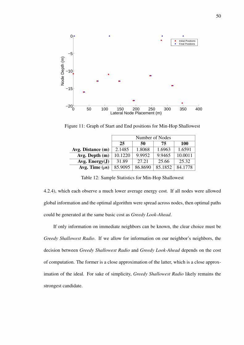
Figure 11: Graph of Start and End positions for Min-Hop Shallowest
Number of Nodes25 50 75 100
Avg. Distance (m) 2.1485 1.8068 1.6963 1.6591Avg. Depth (m) 10.1220 9.9952 9.9465 10.0011Avg. Energy(J) 31.89 27.21 25.66 25.32Avg. Time (µs) 85.9095 86.8690 85.1852 84.1778
Table 12: Sample Statistics for Min-Hop Shallowest
4.2.4), which each observe a much lower average energy cost. If all nodes were allowed
global information and the optimal algorithm were spread across nodes, then optimal paths
could be generated at the same basic cost as Greedy Look-Ahead.
If only information on immediate neighbors can be known, the clear choice must be
Greedy Shallowest Radio. If we allow for information on our neighbor’s neighbors, the
decision between Greedy Shallowest Radio and Greedy Look-Ahead depends on the cost
of computation. The former is a close approximation of the latter, which is a close approx-
imation of the ideal. For sake of simplicity, Greedy Shallowest Radio likely remains the
strongest candidate.
51
Chapter 5: Experiments and Results
In this chapter we discuss the set of experiments we conducted and their results. We
chose to conduct a total of four experiments. The first is using default simulation settings
and across all eight algorithms discussed in Chapter 4. The second explores the effect of
changing how nodes are placed; first by having a fixed maximum distance and moving
the minimum towards it, and then by using a fixed minimum distance and bringing the
maximum down to it. The third uses a fixed radio range, and increases acoustic range up
to the radio capabilities. Lastly, we use a fixed acoustic range, and demonstrate the effect
changes in radio ranges have. We end this chapter with a brief discussion of the results and
draw conclusions on which algorithms are optimal, and how this answer can change.
5.1 Experiments
The simulator requires several settings to be defined beyond the number of nodes and
length of message queues. These settings include minimum and maximum lateral node
placement (by default: 30 to 60 meters apart on the x-axis), minimum and maximum node
depth (ranging from -20m to 0m depth), and the range of the acoustic and radio modems.
It will be noted when these values are modified, the full set of features and default values
can be seen in Appendix A.1.1.
5.1.1 Basic System, All Algorithms. All default values are preserved in this ex-
periment, as described in Table 13. These settings ensure that each node has at least one
52
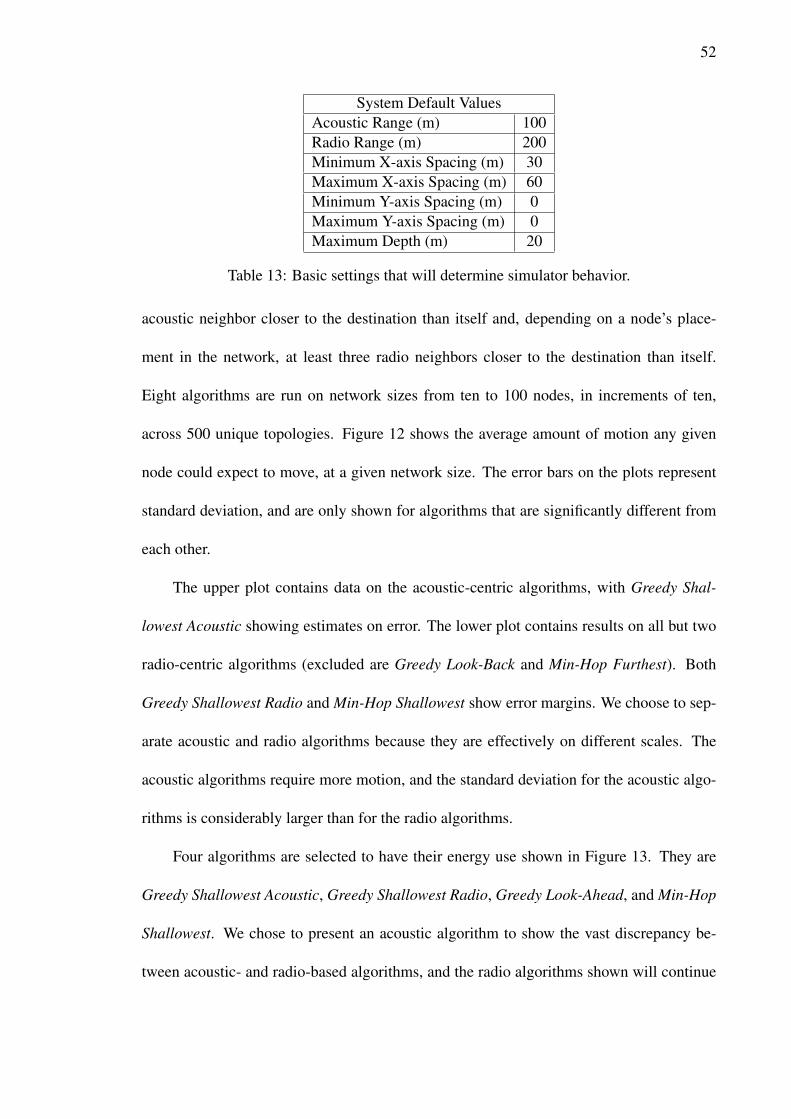
System Default ValuesAcoustic Range (m) 100Radio Range (m) 200Minimum X-axis Spacing (m) 30Maximum X-axis Spacing (m) 60Minimum Y-axis Spacing (m) 0Maximum Y-axis Spacing (m) 0Maximum Depth (m) 20
Table 13: Basic settings that will determine simulator behavior.
acoustic neighbor closer to the destination than itself and, depending on a node’s place-
ment in the network, at least three radio neighbors closer to the destination than itself.
Eight algorithms are run on network sizes from ten to 100 nodes, in increments of ten,
across 500 unique topologies. Figure 12 shows the average amount of motion any given
node could expect to move, at a given network size. The error bars on the plots represent
standard deviation, and are only shown for algorithms that are significantly different from
each other.
The upper plot contains data on the acoustic-centric algorithms, with Greedy Shal-
lowest Acoustic showing estimates on error. The lower plot contains results on all but two
radio-centric algorithms (excluded are Greedy Look-Back and Min-Hop Furthest). Both
Greedy Shallowest Radio and Min-Hop Shallowest show error margins. We choose to sep-
arate acoustic and radio algorithms because they are effectively on different scales. The
acoustic algorithms require more motion, and the standard deviation for the acoustic algo-
rithms is considerably larger than for the radio algorithms.
Four algorithms are selected to have their energy use shown in Figure 13. They are
Greedy Shallowest Acoustic, Greedy Shallowest Radio, Greedy Look-Ahead, and Min-Hop
Shallowest. We chose to present an acoustic algorithm to show the vast discrepancy be-
tween acoustic- and radio-based algorithms, and the radio algorithms shown will continue

53
10 20 30 40 50 60 70 80 90 1000
2
4
6
8
Greedy Furthest AcousticGreedy Shallowest Acoustic
10 20 30 40 50 60 70 80 90 1000
1
2
3
4
5
Number of Nodes
Dis
tanc
e T
rave
lled
(m)
Greedy Shallowest RadioGreedy Furthest RadioMin−Hop ShallowestGreedy Look−Ahead
Figure 12: Graph of Start and End positions for Greedy Furthest Acoustic
30 60 900
20
40
60
80
100
Number of Nodes
Ene
rgy
Con
sum
ed (
J)
Greedy Shallowest AcousticGreedy Shallowest RadioGreedy Look−AheadMin−Hop Shallowest
Figure 13: Graph of Energy Consumed by Four Algorithms
54
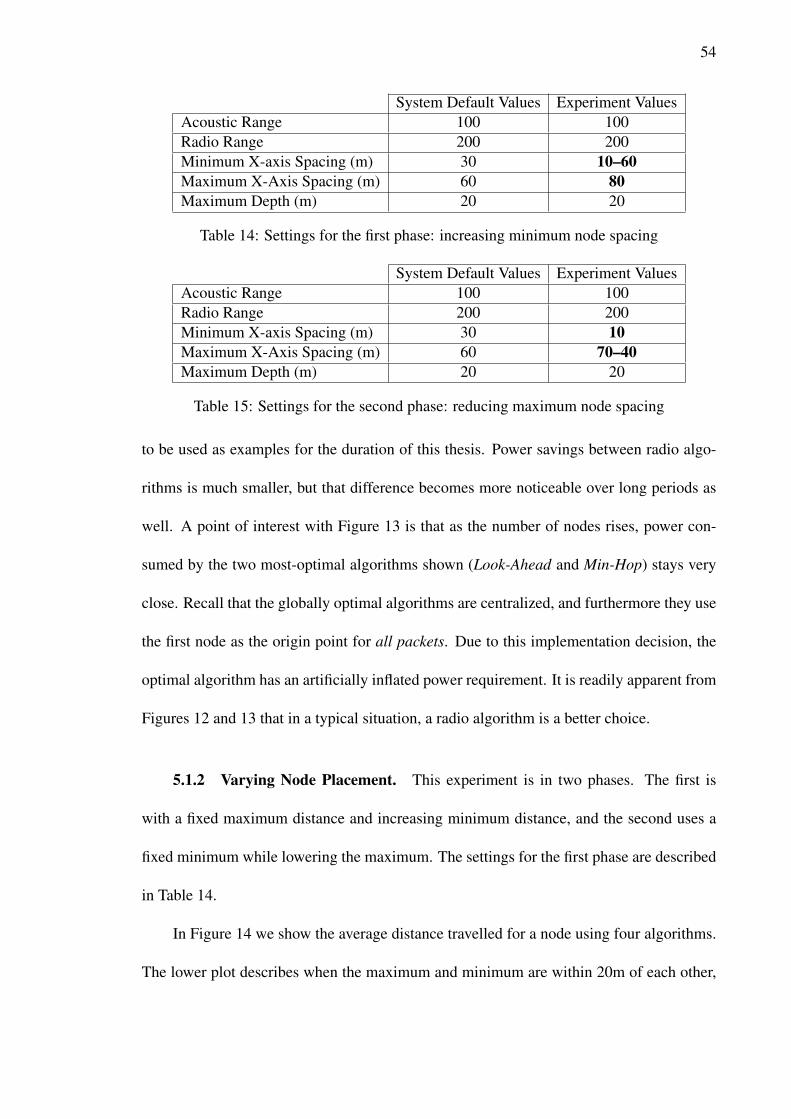
System Default Values Experiment ValuesAcoustic Range 100 100Radio Range 200 200Minimum X-axis Spacing (m) 30 10–60Maximum X-Axis Spacing (m) 60 80Maximum Depth (m) 20 20
Table 14: Settings for the first phase: increasing minimum node spacing
System Default Values Experiment ValuesAcoustic Range 100 100Radio Range 200 200Minimum X-axis Spacing (m) 30 10Maximum X-Axis Spacing (m) 60 70–40Maximum Depth (m) 20 20
Table 15: Settings for the second phase: reducing maximum node spacing
to be used as examples for the duration of this thesis. Power savings between radio algo-
rithms is much smaller, but that difference becomes more noticeable over long periods as
well. A point of interest with Figure 13 is that as the number of nodes rises, power con-
sumed by the two most-optimal algorithms shown (Look-Ahead and Min-Hop) stays very
close. Recall that the globally optimal algorithms are centralized, and furthermore they use
the first node as the origin point for all packets. Due to this implementation decision, the
optimal algorithm has an artificially inflated power requirement. It is readily apparent from
Figures 12 and 13 that in a typical situation, a radio algorithm is a better choice.
5.1.2 Varying Node Placement. This experiment is in two phases. The first is
with a fixed maximum distance and increasing minimum distance, and the second uses a
fixed minimum while lowering the maximum. The settings for the first phase are described
in Table 14.
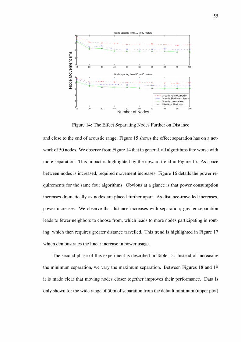
In Figure 14 we show the average distance travelled for a node using four algorithms.
The lower plot describes when the maximum and minimum are within 20m of each other,
55
10 20 30 40 50 60 70 80 90 1000
1
2
3
4Node spacing from 10 to 80 meters
10 20 30 40 50 60 70 80 90 1000
1
2
3
4
5Node spacing from 50 to 80 meters
Number of Nodes
Nod
e M
ovem
ent (
m)
Greedy Furthest RadioGreedy Shallowest RadioGreedy Look−AheadMin−Hop Shallowest
Figure 14: The Effect Separating Nodes Further on Distance
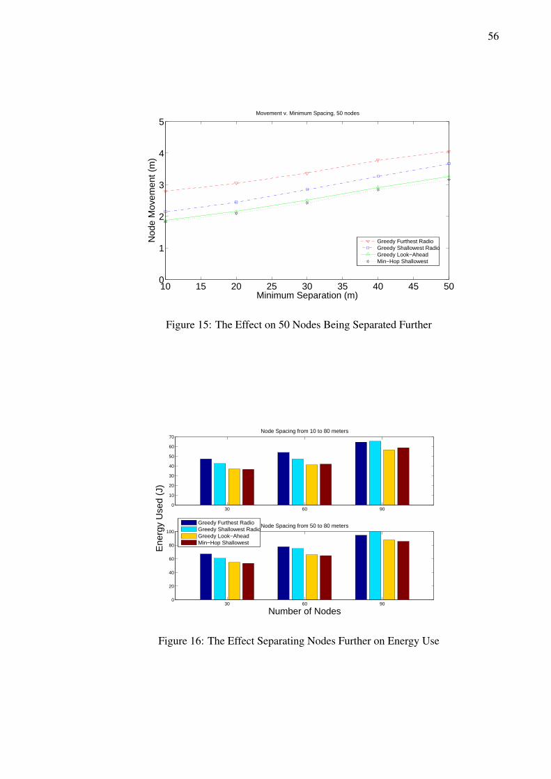
and close to the end of acoustic range. Figure 15 shows the effect separation has on a net-
work of 50 nodes. We observe from Figure 14 that in general, all algorithms fare worse with
more separation. This impact is highlighted by the upward trend in Figure 15. As space
between nodes is increased, required movement increases. Figure 16 details the power re-
quirements for the same four algorithms. Obvious at a glance is that power consumption
increases dramatically as nodes are placed further apart. As distance-travelled increases,
power increases. We observe that distance increases with separation; greater separation
leads to fewer neighbors to choose from, which leads to more nodes participating in rout-
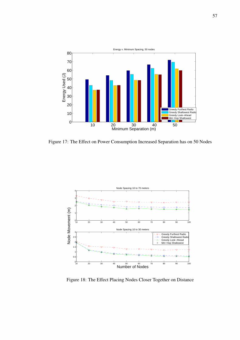
ing, which then requires greater distance travelled. This trend is highlighted in Figure 17
which demonstrates the linear increase in power usage.
The second phase of this experiment is described in Table 15. Instead of increasing
the minimum separation, we vary the maximum separation. Between Figures 18 and 19
it is made clear that moving nodes closer together improves their performance. Data is
only shown for the wide range of 50m of separation from the default minimum (upper plot)
56
10 15 20 25 30 35 40 45 500
1
2
3
4
5Movement v. Minimum Spacing, 50 nodes
Minimum Separation (m)
Nod
e M
ovem
ent (
m)
Greedy Furthest RadioGreedy Shallowest RadioGreedy Look−AheadMin−Hop Shallowest
Figure 15: The Effect on 50 Nodes Being Separated Further
30 60 900
10
20
30
40
50
60
70Node Spacing from 10 to 80 meters
30 60 900
20
40
60
80
100Node Spacing from 50 to 80 meters
Number of Nodes
Ene
rgy
Use
d (J
)
Greedy Furthest RadioGreedy Shallowest RadioGreedy Look−AheadMin−Hop Shallowest
Figure 16: The Effect Separating Nodes Further on Energy Use
57
10 20 30 40 500
10
20
30
40
50
60
70
80Energy v. Minimum Spacing, 50 nodes
Minimum Separation (m)
Ene
rgy
Use
d (J
)
Greedy Furthest RadioGreedy Shallowest RadioGreedy Look−AheadMin−Hop Shallowest
Figure 17: The Effect on Power Consumption Increased Separation has on 50 Nodes
10 20 30 40 50 60 70 80 90 1000
1
2
3
4Node Spacing 10 to 70 meters
10 20 30 40 50 60 70 80 90 1000
0.5
1
1.5
2
2.5
3
Node Spacing 10 to 30 meters
Number of Nodes
Nod
e M
ovem
ent (
m)
Greedy Furthest RadioGreedy Shallowest RadioGreedy Look−AheadMin−Hop Shallowest
Figure 18: The Effect Placing Nodes Closer Together on Distance
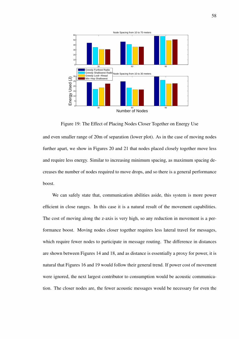
58
30 60 900
10
20
30
40
50
60Node Spacing from 10 to 70 meters
30 60 900
5
10
15
20
25
30Node Spacing from 10 to 30 meters
Number of Nodes
Ene
rgy
Use
d (J
)
Greedy Furthest RadioGreedy Shallowest RadioGreedy Look−AheadMin−Hop Shallowest
Figure 19: The Effect of Placing Nodes Closer Together on Energy Use
and even smaller range of 20m of separation (lower plot). As in the case of moving nodes
further apart, we show in Figures 20 and 21 that nodes placed closely together move less
and require less energy. Similar to increasing minimum spacing, as maximum spacing de-
creases the number of nodes required to move drops, and so there is a general performance
boost.
We can safely state that, communication abilities aside, this system is more power
efficient in close ranges. In this case it is a natural result of the movement capabilities.
The cost of moving along the z-axis is very high, so any reduction in movement is a per-
formance boost. Moving nodes closer together requires less lateral travel for messages,
which require fewer nodes to participate in message routing. The difference in distances
are shown between Figures 14 and 18, and as distance is essentially a proxy for power, it is
natural that Figures 16 and 19 would follow their general trend. If power cost of movement
were ignored, the next largest contributor to consumption would be acoustic communica-
tion. The closer nodes are, the fewer acoustic messages would be necessary for even the
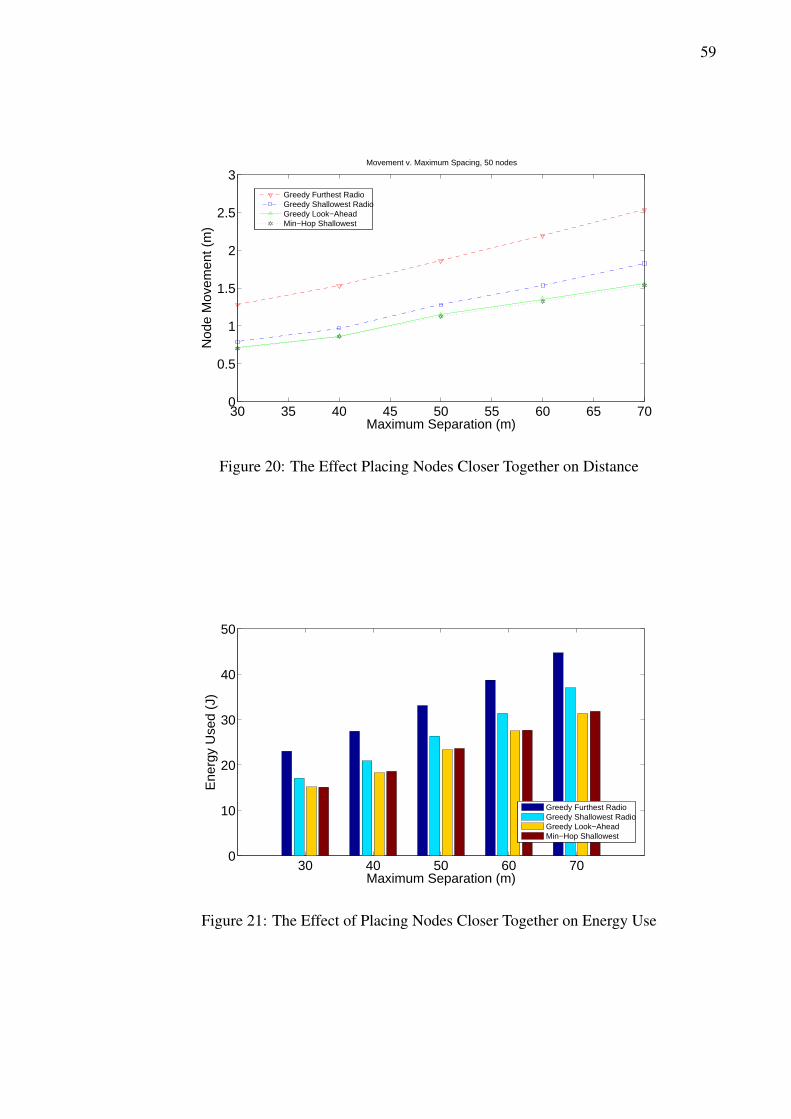
59
30 35 40 45 50 55 60 65 700
0.5
1
1.5
2
2.5
3
Maximum Separation (m)
Nod
e M
ovem
ent (
m)
Movement v. Maximum Spacing, 50 nodes
Greedy Furthest RadioGreedy Shallowest RadioGreedy Look−AheadMin−Hop Shallowest
Figure 20: The Effect Placing Nodes Closer Together on Distance
30 40 50 60 700
10
20
30
40
50
Maximum Separation (m)
Ene
rgy
Use
d (J
)
Greedy Furthest RadioGreedy Shallowest RadioGreedy Look−AheadMin−Hop Shallowest
Figure 21: The Effect of Placing Nodes Closer Together on Energy Use
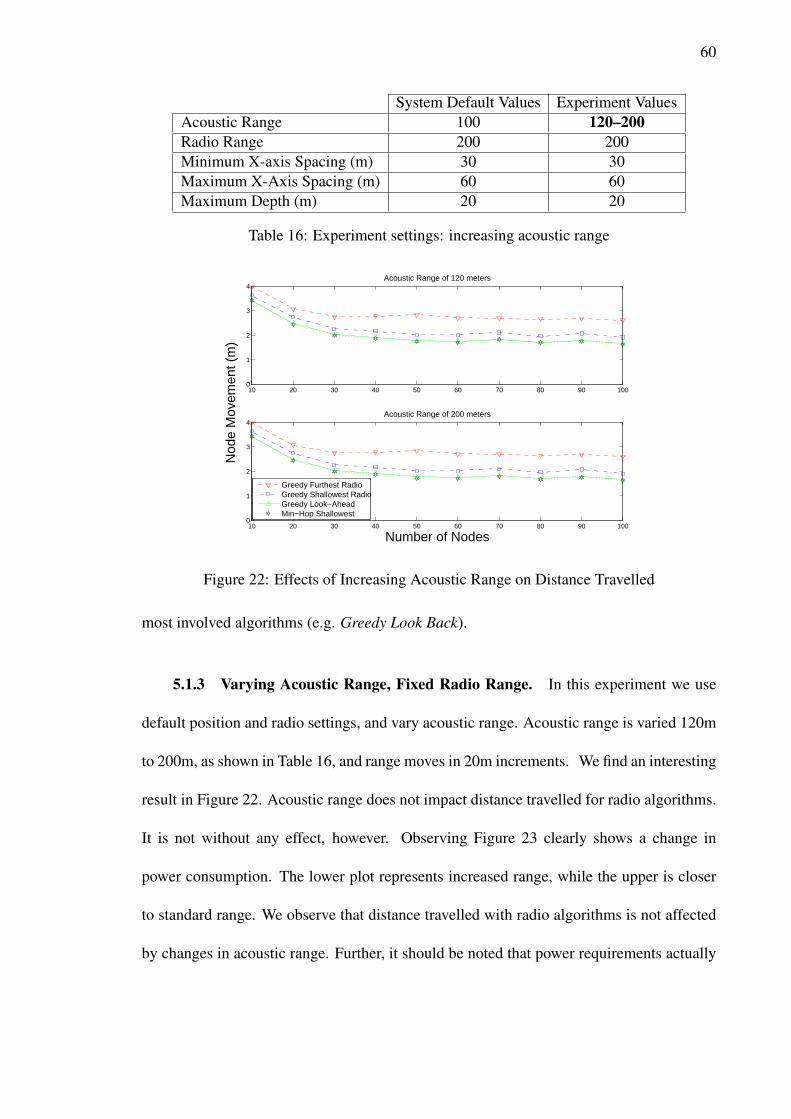
60
System Default Values Experiment ValuesAcoustic Range 100 120–200Radio Range 200 200Minimum X-axis Spacing (m) 30 30Maximum X-Axis Spacing (m) 60 60Maximum Depth (m) 20 20
Table 16: Experiment settings: increasing acoustic range
10 20 30 40 50 60 70 80 90 1000
1
2
3
4Acoustic Range of 120 meters
10 20 30 40 50 60 70 80 90 1000
1
2
3
4Acoustic Range of 200 meters
Number of Nodes
Nod
e M
ovem
ent (
m)
Greedy Furthest RadioGreedy Shallowest RadioGreedy Look−AheadMin−Hop Shallowest
Figure 22: Effects of Increasing Acoustic Range on Distance Travelled
most involved algorithms (e.g. Greedy Look Back).
5.1.3 Varying Acoustic Range, Fixed Radio Range. In this experiment we use
default position and radio settings, and vary acoustic range. Acoustic range is varied 120m
to 200m, as shown in Table 16, and range moves in 20m increments. We find an interesting
result in Figure 22. Acoustic range does not impact distance travelled for radio algorithms.
It is not without any effect, however. Observing Figure 23 clearly shows a change in
power consumption. The lower plot represents increased range, while the upper is closer
to standard range. We observe that distance travelled with radio algorithms is not affected
by changes in acoustic range. Further, it should be noted that power requirements actually
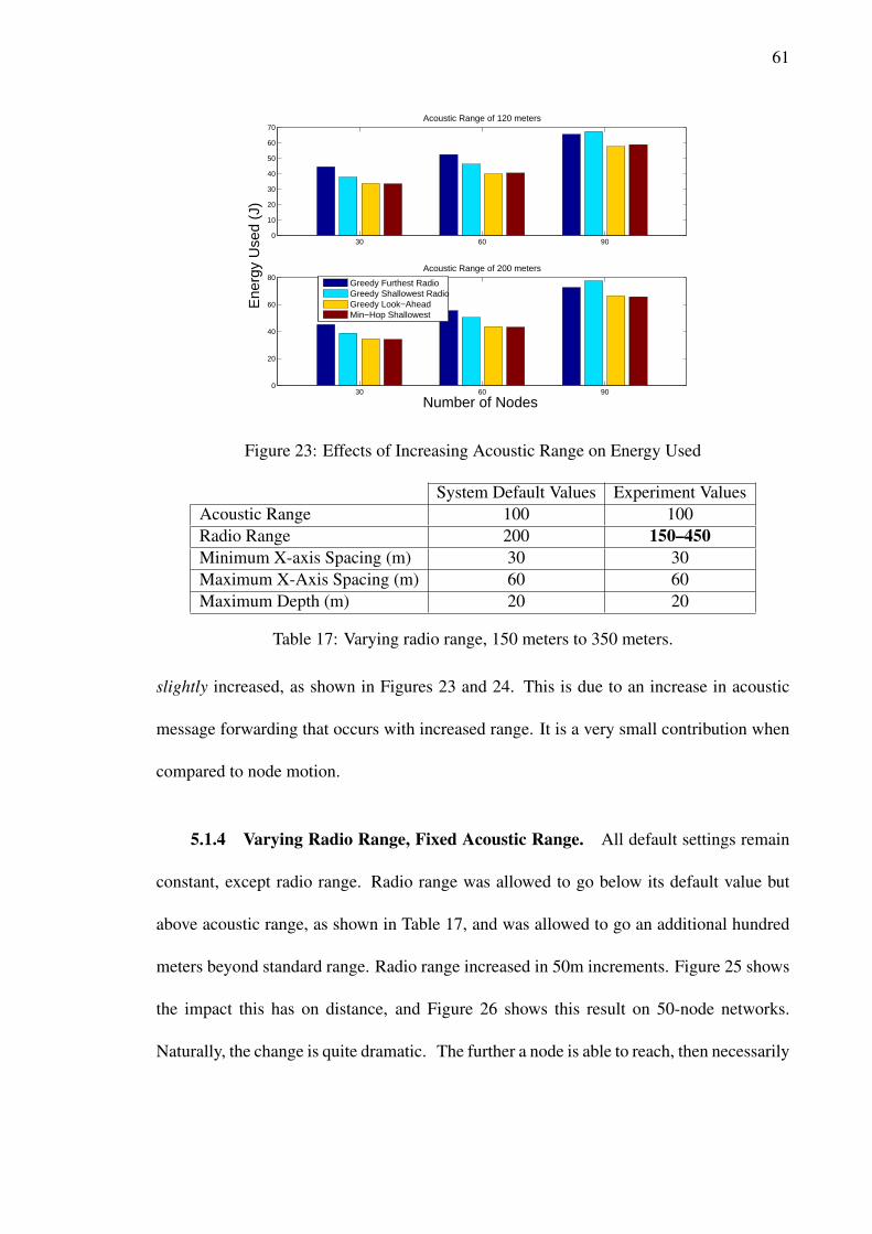
61
30 60 900
10
20
30
40
50
60
70Acoustic Range of 120 meters
Number of Nodes
Ene
rgy
Use
d (J
)
30 60 900
20
40
60
80Acoustic Range of 200 meters
Greedy Furthest RadioGreedy Shallowest RadioGreedy Look−AheadMin−Hop Shallowest
Figure 23: Effects of Increasing Acoustic Range on Energy Used
System Default Values Experiment ValuesAcoustic Range 100 100Radio Range 200 150–450Minimum X-axis Spacing (m) 30 30Maximum X-Axis Spacing (m) 60 60Maximum Depth (m) 20 20
Table 17: Varying radio range, 150 meters to 350 meters.
slightly increased, as shown in Figures 23 and 24. This is due to an increase in acoustic
message forwarding that occurs with increased range. It is a very small contribution when
compared to node motion.
5.1.4 Varying Radio Range, Fixed Acoustic Range. All default settings remain
constant, except radio range. Radio range was allowed to go below its default value but
above acoustic range, as shown in Table 17, and was allowed to go an additional hundred
meters beyond standard range. Radio range increased in 50m increments. Figure 25 shows
the impact this has on distance, and Figure 26 shows this result on 50-node networks.
Naturally, the change is quite dramatic. The further a node is able to reach, then necessarily
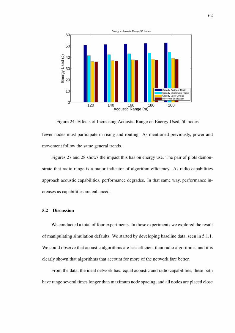
62
120 140 160 180 2000
10
20
30
40
50
60
Acoustic Range (m)
Ene
rgy
Use
d (J
)
Energy v. Acoustic Range, 50 Nodes
Greedy Furthest RadioGreedy Shallowest RadioGreedy Look−AheadMin−Hop Shallowest
Figure 24: Effects of Increasing Acoustic Range on Energy Used, 50 nodes
fewer nodes must participate in rising and routing. As mentioned previously, power and
movement follow the same general trends.
Figures 27 and 28 shows the impact this has on energy use. The pair of plots demon-
strate that radio range is a major indicator of algorithm efficiency. As radio capabilities
approach acoustic capabilities, performance degrades. In that same way, performance in-
creases as capabilities are enhanced.
5.2 Discussion
We conducted a total of four experiments. In those experiments we explored the result
of manipulating simulation defaults. We started by developing baseline data, seen in 5.1.1.
We could observe that acoustic algorithms are less efficient than radio algorithms, and it is
clearly shown that algorithms that account for more of the network fare better.
From the data, the ideal network has: equal acoustic and radio capabilities, these both
have range several times longer than maximum node spacing, and all nodes are placed close
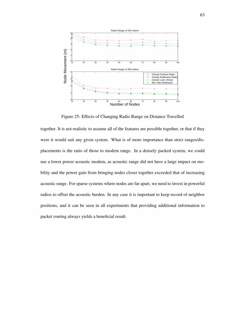
63
10 20 30 40 50 60 70 80 90 1000
1
2
3
4
5Radio Range of 150 meters
10 20 30 40 50 60 70 80 90 1000
1
2
3
4Radio Range of 350 meters
Number of Nodes
Nod
e M
ovem
ent (
m)
Greedy Furthest RadioGreedy Shallowest RadioGreedy Look−AheadMin−Hop Shallowest
Figure 25: Effects of Changing Radio Range on Distance Travelled
together. It is not realistic to assume all of the features are possible together, or that if they
were it would suit any given system. What is of more importance than strict ranges/dis-
placements is the ratio of those to modem range. In a densely packed system, we could
use a lower power acoustic modem, as acoustic range did not have a large impact on mo-
bility and the power gain from bringing nodes closer together exceeded that of increasing
acoustic range. For sparse systems where nodes are far apart, we need to invest in powerful
radios to offset the acoustic burden. In any case it is important to keep record of neighbor
positions, and it can be seen in all experiments that providing additional information to
packet routing always yields a beneficial result.

64
150 200 250 300 3500
0.5
1
1.5
2
2.5
3
3.5
4
Radio Range (m)
Nod
e M
ovem
ent (
m)
Movement v. Radio Range, 50 Nodes
Greedy Furthest RadioGreedy Shallowest RadioGreedy Look−AheadMin−Hop Shallowest
Figure 26: Effects of Changing Radio Range on Distance Travelled for 50-Node Networks
30 60 900
20
40
60
80
100Radio Range of 150 meters
30 60 900
10
20
30
40Radio Range of 350 meters
Number of Nodes
Ene
rgy
Use
d (J
)
Greedy Furthest RadioGreedy Shallowest RadioGreedy Look−AheadMin−Hop Shallowest
Figure 27: Effects of Changing Radio Range on Energy Used

65
150 200 250 300 3500
10
20
30
40
50
60
70Energy v. Radio Range, 50 Nodes
Radio Range (m)
Ene
rgy
Use
d (J
)
Greedy Furthest RadioGreedy Shallowest RadioGreedy Look−AheadMin−Hop Shallowest
Figure 28: Effects of Changing Radio Range on Energy Used
66
Chapter 6: Conclusions
Networking and routing are problems that have been solved on land years ago, but
due to the unique constraints of the underwater environment we must solve them again.
This is a fledgeling field, so we assist in this endeavor by developing an analytical tool
and describing who should participate in routing. To that end we developed a simulation
environment in MATLAB, and implemented eight algorithms to make the participation de-
cision. Between those algorithms and the behavior of the simulator, we provide suggested
approaches to managing radio use. A large number of test cases were required to verify the
accuracy as can be seen in chapter 5, but we are confident in our recommendations.
6.1 Summary In Brief
Using MATLAB we developed a set of scripts and functions that replicated the basic
functionality of an AquaNode [1] in an idealized environment. We assume perfect com-
munication, and we do not presently allow for a node to be temporarily or permanently
disabled. Within this ideal system, where energy is consumed and tracked but not limited,
we develop and test eight algorithms. Two of them were based on the acoustic capabili-
ties, the other six based on radio capabilities. The acoustic-algorithms and first two radio-
algorithms share the same decision process. They are ”furthest neighbor” and ”shallowest
neighbor” approaches. We show that using the radio approach is more effective as long
as the range of the radio is greater than acoustic range, and as their ranges come closer
67
together we see their performances converging.
The primary lesson learned is that radio-centric algorithms are generally more effi-
cient, and the more information available allows for more economic motion and power
consumption. If an agent only knows the positions of its neighbors, Greedy Shallowest
Radio is the best choice. If processing power is available and we have information on our
neighbors and their neighbors, Greedy Look-Ahead is the best choice, assuming we don’t
want a centralized approach. These two algorithms allow for a fully distributed approach
using local or semi-local information only.
6.2 Contributions
We have two main contributions. The first is the creation of an aquatic simulator that
allows for rapid prototyping and validation of algorithms. The second is the evaluation of
basic schemes that can be readily implemented on a physical system, while providing a
rough estimate of their efficacy.
As stated in Chapter 1, we developed an environment based on AquaNodes. The sys-
tem is implemented in MATLAB, so development times are very short. This allowed us
and can allow others to quickly create, test, and modify algorithms and simulator exten-
sions. We demonstrate this through the algorithms we implemented. Each of them were
implemented in an abstract fashion which allowed for proof of concept. The abstract imple-
mentation demonstrates how the real system should behave, and so provides a framework
to progress in more physical versions.

68
6.3 Future Work
There are two primary ways the work of this thesis can be extended. The first is by
extending the capabilities of the simulator itself. The second is through implementing the
algorithms on a physical system.
Some ways the simulator could be expanded are: allowing node sleep or power loss,
implementing the behavior of the AquaNode multiprocessor system (including variable
power requirements), and implementing communication interference. Sleeping nodes and
the multiprocessor system would allow for more realism in power consumption, and thus
the trends we show in chapter 5 would be more assuredly held to, and any power saving ef-
forts could be tested in a time-accelerated environment. Interference takes multiple forms.
The first is by varying the success rate of communication to serve as a proxy for general
conditions. Data for this is available in [1]. The simulator could be further expanded to
having environmental settings, such as the existence and persistence of thermoclines. A
truly accurate system would track the acoustic power of all relevant transmissions and de-
termine simple noise-interference from other nodes “talking” or messages reflecting off of
surfaces.
The goal of this thesis has been to develop a simulation environment and a sample set
of algorithms for evaluation. It is our sincere hope that this tool will be of use to researchers
working on wireless underwater networks. There are many new and exciting approaches to
the problems aquatic systems face, and we hope we’ve made the process of exploring these
approaches a little easier. It is critical we properly develop and leverage aquatic technology
so we can understand and make use of what the ocean provides.
69
REFERENCES
[1] C. Detweiler, Decentralized Sensor Placement and Mobile Localization on an Un-
derwater Sensor Network with Depth Adjustment Capabilities. PhD thesis, Mas-
sachusetts Institute of Technology, Cambridge, MA, USA, July 2010.
[2] C. Detweiler, M. Doniec, I. Vasilescu, E. Basha, and D. Rus, “Autonomous depth
adjustment for underwater sensor networks,” in Proc. of the Intl Workshop on Under-
Water Networks (WUWNet), p. 12:112:4, 2010.
[3] C. Detweiler, M. Doniec, I. Vasilescu, and D. Rus, “Autonomous depth adjustment
for underwater sensor networks: Design and applications,” IEEE Transactions on
Mechatronics, vol. 17, no. 1, pp. 16–24, 2012.
[4] I. Vasilescu, Using Light Underwater: Devices, Algorithms and Systems for Maritime
Persistent Surveillance. PhD thesis, MIT, 2009.
[5] M. O’Rourke, E. Basha, and C. Detweiler, “Multi-modal communications in under-
water sensor networks using depth adjustment,” (Los Angeles, CA, USA), 2012.
[6] C. Chen and J. Ma, “Mobile enabled large scale wireless sensor networks,” in Ad-
vanced Communication Technology, 2006. ICACT 2006. The 8th International Con-
ference, vol. 1, p. 333338, 2006.
[7] S. Krco, D. Cleary, and D. Parker, “P2P mobile sensor networks,” in System Sciences,
70
2005. HICSS’05. Proceedings of the 38th Annual Hawaii International Conference
on, p. 324c, 2005.
[8] I. F. Akyildiz, D. Pompili, and T. Melodia, “State-of-the-art in protocol research for
underwater acoustic sensor networks,” in Proc. of the 1st WUWNet, (Los Angeles,
CA, USA), p. 716, 2006.
[9] J. Rice, “SeaWeb acoustic communication and navigation networks,” in Proceedings
of the International Conference on Underwater Acoustic Measurements: Technolo-
gies and Results, 2005.
[10] J.-H. Cui, J. Kong, M. Gerla, and S. Zhou, “The challenges of building mobile under-
water wireless networks for aquatic applications,” Network, IEEE, vol. 20, p. 1218,
June 2006.
[11] Z. Zhou, H. Yan, S. Ibrahim, J.-H. Cui, Z. Shi, and R. Ammar, “Enhancing under-
water acoustic sensor networks using surface radios: Issues, challenges and solu-
tions,” in Sensor Networks (G. Ferrari, ed.), Signals and Communication Technology,
p. 283307, Springer Berlin Heidelberg, 2009.
[12] B. Chen, P. C. Hickey, and D. Pompili, “Trajectory-aware communication solution
for underwater gliders using WHOI micro-modems,” in Sensor Mesh and Ad Hoc
Communications and Networks (SECON), 2010 7th Annual IEEE Communications
Society Conference on, p. 19, 2010.
[13] N. Arad and Y. Shavitt, “Minimizing recovery state in geographic ad-hoc routing,” in
Proceedings of the 7th ACM international symposium on Mobile ad hoc networking
and computing, MobiHoc ’06, (New York, NY, USA), p. 1324, ACM, 2006.

71
[14] G. Tan, M. Bertier, and A.-M. Kermarrec, “Visibility-graph-based shortest-path ge-
ographic routing in sensor networks,” in INFOCOM 2009, IEEE, p. 17191727, Apr.
2009.
[15] Z.-Y. He and P. Jiang, “Design of wireless gateway based on ZigBee and GPRS tech-
nology,” in 2009 International Conference on Computational Intelligence and Soft-
ware Engineering, (Wuhan, China), pp. 1–4, Dec. 2009.
[16] H.-j. He, Z.-q. Yue, and X.-j. Wang, “Design and realization of wireless sensor net-
work gateway based on ZigBee and GPRS,” in 2009 Second International Conference
on Information and Computing Science, (Manchester, England, UK), pp. 196–199,
May 2009.
[17] S. Chumkamon, P. Tuvaphanthaphiphat, and P. Keeratiwintakorn, “The vertical hand-
off between GSM and zigbee networks for vehicular communication,” in Electrical
Engineering/Electronics Computer Telecommunications and Information Technology
(ECTI-CON), 2010 International Conference on, p. 603606, 2010.
[18] S. Lin, S. xiangquan, and L. Ming, “A wireless network based on the combination of
zigbee and GPRS,” in 2008 IEEE International Conference on Networking, Sensing
and Control, (Sanya, China), pp. 267–270, Apr. 2008.
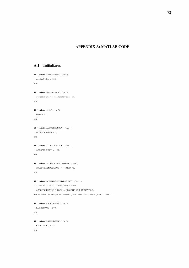
72
APPENDIX A: MATLAB CODE
A.1 Initializers
i f ˜ e x i s t ( ’ numberNodes ’ , ’ v a r ’ )
numberNodes = 100 ;
end
i f ˜ e x i s t ( ’ queueLength ’ , ’ v a r ’ )
queueLength = c e i l ( numberNodes / 2 ) ;
end
i f ˜ e x i s t ( ’mode ’ , ’ v a r ’ )
mode = 8 ;
end
i f ˜ e x i s t ( ’ACOUSTIC INDEX ’ , ’ v a r ’ )
ACOUSTIC INDEX = 2 ;
end
i f ˜ e x i s t ( ’ACOUSTIC RANGE ’ , ’ v a r ’ )
ACOUSTIC RANGE = 100 ;
end
i f ˜ e x i s t ( ’ACOUSTIC SEND ENERGY ’ , ’ v a r ’ )
ACOUSTIC SEND ENERGY= 0 . 1 1 3 6 / 1 0 0 0 ;
end
i f ˜ e x i s t ( ’ACOUSTIC RECEIVE ENERGY ’ , ’ v a r ’ )
% e s t i m a t e u n t i l I have r e a l v a l u e s
ACOUSTIC RECEIVE ENERGY = ACOUSTIC SEND ENERGY / 1 . 8 ;
end % based o f change i n c u r r e n t from D e t w e i l e r t h e s i s p . 7 1 , t a b l e 3 . 1
i f ˜ e x i s t ( ’RADIO RANGE ’ , ’ v a r ’ )
RADIO RANGE = 200 ;
end
i f ˜ e x i s t ( ’RADIO INDEX ’ , ’ v a r ’ )
RADIO INDEX = 1 ;
end
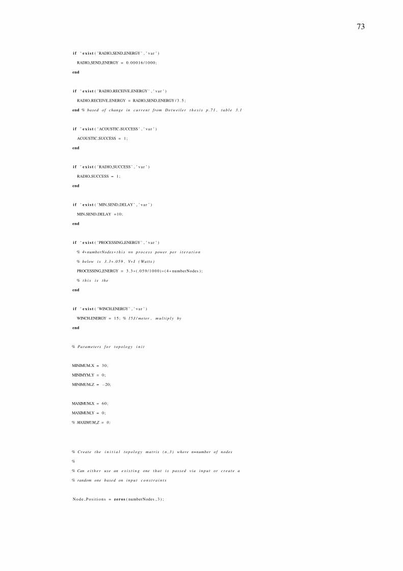
73
i f ˜ e x i s t ( ’RADIO SEND ENERGY ’ , ’ v a r ’ )
RADIO SEND ENERGY = 0 . 0 0 0 1 6 / 1 0 0 0 ;
end
i f ˜ e x i s t ( ’RADIO RECEIVE ENERGY ’ , ’ v a r ’ )
RADIO RECEIVE ENERGY = RADIO SEND ENERGY / 3 . 5 ;
end % based o f change i n c u r r e n t from D e t w e i l e r t h e s i s p . 7 1 , t a b l e 3 . 1
i f ˜ e x i s t ( ’ACOUSTIC SUCCESS ’ , ’ v a r ’ )
ACOUSTIC SUCCESS = 1 ;
end
i f ˜ e x i s t ( ’RADIO SUCCESS ’ , ’ v a r ’ )
RADIO SUCCESS = 1 ;
end
i f ˜ e x i s t ( ’MIN SEND DELAY ’ , ’ v a r ’ )
MIN SEND DELAY =10;
end
i f ˜ e x i s t ( ’PROCESSING ENERGY ’ , ’ v a r ’ )
% 4∗ numberNodes∗ t h i s == p r o c e s s power per i t e r a t i o n
% below i s 3 . 3∗ . 0 5 9 , V∗ I ( Wat t s )
PROCESSING ENERGY = 3 . 3 ∗ ( . 0 5 9 / 1 0 0 0 ) ∗ ( 4 ∗ numberNodes ) ;
% t h i s i s t h e
end
i f ˜ e x i s t ( ’WINCH ENERGY ’ , ’ v a r ’ )
WINCH ENERGY = 1 5 ; % 15 J / meter , m u l t i p l y by
end
% Parame ter s f o r t o p o l o g y i n i t
MINIMUM X = 3 0 ;
MINIMYM Y = 0 ;
MINIMUM Z = −20;
MAXIMUM X = 6 0 ;
MAXIMUM Y = 0 ;
% MAXIMUM Z = 0;
% Cr ea t e t h e i n i t i a l t o p o l o g y m a t r i x ( n , 3 ) where n=number o f nodes
%
% Can e i t h e r use an e x i s t i n g one t h a t i s p as sed v i a i n p u t or c r e a t e a
% random one based on i n p u t c o n s t r a i n t s
N o d e P o s i t i o n s = z e r o s ( numberNodes , 3 ) ;
74
i f e x i s t ( ’ N o d e P o s i t i o n s ’ , ’ v a r ’ )
numberNodes = l e n g t h ( N o d e P o s i t i o n s ( : , 1 ) ) ;
e l s e
N o d e P o s i t i o n s = z e r o s ( numberNodes , 3 ) ;
p r ev = [0 0 0 ] ;
f o r i =1 : numberNodes
x = 0 ;
y = 0 ;
z = 0 ;
whi le x < MINIMUM X | | x > MAXIMUM X
i f i == 1
x = 0 ;
break ;
end
x = rand ( 1 )∗MAXIMUM X;
end
x = x + prev ( 1 ) ;
% w h i l e y < MINIMYM Y | | y > MAXIMUM Y
% y = rand ( 1 )∗MAXIMUM Y;
% end
% y = y + prev ( 2 ) ;
y = 0 ;
%
% Z o p e r a t e s on n e g a t i v e s , so we go from max ( assumed 0) t o min
% T h i s means we go from a n e g a t i v e t o z e r o . J u s t l o o k a t t h e code !
z = rand ( 1 )∗MINIMUM Z ;
%
%
%
p rev = [ x y z ] ;
N o d e P o s i t i o n s ( i , : ) = p rev ;
end
end
c l e a r i x y z p rev
% c l e a r MAXIMUM X MAXIMUM Y %MAXIMUM Z
% c l e a r MINIMUM X MINIMYM Y MINIMUM Z
% Cr ea t e c o n n e c t i v i t y m a t r i x based on t o p o l o g y
%
<<<<<<< l o c a l
% I n p u t s : N o d e P o s i t i o n s , numberNodex
=======
% I n p u t s : N o d e P o s i t i o n s , ACOUSTIC RANGE , RADIO RANGE , RADIO INDEX , ACOUSTIC INDEX
>>>>>>> o t h e r
75
% O u t p u t s : C o n n e c t i v i t y M a t r i x
% Cr ea t e empty m a t r i x
C o n n e c t i v i t y M a t r i x = z e r o s ( numberNodes , numberNodes , 2 ) ;
% Fi gu re o u t n e i g h b o r s f o r bo th communica t ion t y p e s
C o n n e c t i v i t y M a t r i x ( : , : , RADIO INDEX ) = s q u a r e f o r m ( p d i s t ( N o d e P o s i t i o n s ( : , 1 ) ) ) ;
C o n n e c t i v i t y M a t r i x ( : , : , ACOUSTIC INDEX ) = s q u a r e f o r m ( p d i s t ( N o d e P o s i t i o n s ( : , 1 : 2 ) ) ) ;
f o r i = 1 : l e n g t h ( C o n n e c t i v i t y M a t r i x ( : , : , RADIO INDEX ) )
f o r j = 1 : l e n g t h ( C o n n e c t i v i t y M a t r i x ( : , : , RADIO INDEX ) )
i f ( C o n n e c t i v i t y M a t r i x ( i , j , RADIO INDEX ) > RADIO RANGE)
C o n n e c t i v i t y M a t r i x ( i , j , RADIO INDEX ) = 0 ;
end
i f ( C o n n e c t i v i t y M a t r i x ( i , j , ACOUSTIC INDEX ) > ACOUSTIC RANGE)
C o n n e c t i v i t y M a t r i x ( i , j , ACOUSTIC INDEX ) = 0 ;
end
end
end
% Ensure l o g i c a l form t o m a t r i x i n s t e a d o f numer ic
C o n n e c t i v i t y M a t r i x = l o g i c a l ( C o n n e c t i v i t y M a t r i x ) ;
c l e a r i j
% Hard w i r i n g f o r t h e s i s r i g h t now
%
%
% NOTE: Read p o i n t e r and w r i t e p o i n t e r are f o r b i d d e n from b e i n g t h e same
% e x c e p t a t t h e s t a r t where t h e y are bo th 1 . A f t e r t h a t , t h e y are n e v e r
% a l l o w e d t o have t h e same v a l u e . T h i s s i m p l i f i e s m o d i f i c a t i o n l o g i c
% b u t r e q u i r e s us t o have a queue l e n g t h 1 more than n e c e s s a r y t o make
% up f o r t h e ” l o s s ” o f a c e l l when t h e y c o u l d be e q u a l .
% Queue l e n g t h s u g g e s t e d t o be number o f nodes or g r e a t e r
i f ˜ ( e x i s t ( ’ queueLength ’ , ’ v a r ’ ) )
queueLength = numberNodes ;
end
% F o l l o w i n g Nick ’ s lead , p a c k e t s w i l l be r e p r e s e n t e d as
% a 1 x4 c e l l array , w i t h each f i e l d b e i n g : Dst , Src , P r o t o c l , Data
% P a c k e t s :
% Dst Src P r o t o c o l Data
% P ac ke t {1 x4} = {} {} {} {}
P a c k e t = c e l l ( 1 , 4 ) ;
76
% t h e f o l l o w i n g m a t r i c e s are ”two pages ” each . Page 1 i s rad io , page 2 i s
% a c o u s t i c .
txQueue = c e l l ( numberNodes , queueLength + 1 , 2 ) ;
rxQueue = c e l l ( numberNodes , queueLength + 1 , 2 ) ;
% I m p l e m e n t a t i o n o f b u f f e r i n g .
% e a v e r y node w i l l read from i t s rxQueue , and w r i t e t o i t s txQueue
% a n o t h e r s c r i p t w i l l h and l e t h e j u g g l i n g o f messages from t x t o rx .
t x Q u e u e P o i n t e r s = ones ( numberNodes , 2 , 2 ) ;
r x Q u e u e P o i n t e r s = ones ( numberNodes , 2 , 2 ) ;
% t h e s e a r r a y s w i l l s t o r e read and w r i t e p o i n t e r s
% as usua l , t h e row i n d i c a t e s t h e node b e i n g r e f e r e n c e d
% I s u g g e s t t h e c o n v e n t i o n o f [ read , w r i t e ] , t x Q u e u e P o i n t e r s [ 1 , 1 ] i s
% txQueue read p o i n t e r f o r node 1 .
% t h e r e i s n o t h i n g wrong w i t h l e a v i n g queues empty f o r now . C e l l s
% are b a s i c a l l y pre−a l l o c a t e d b l o c k s o f memory . F i l l i n g them now or l a t e r
% makes no d i f f e r e n c e . A v a r i a b l e may o n l y t a k e a few b y t e s , b u t t h e overhead
% r e q u i r e d o f a c e l l c o u l d make s t o r i n g t h a t v a l u e i n a c e l l a m a t t e r o f
% k i l o b y t e s .
messagesSen tAndRece ived = z e r o s ( numberNodes , 2 , 2 ) ;
A.2 Main Body
S t a r t P o s i t i o n s = N o d e P o s i t i o n s ;
energyUsed = z e r o s ( numberNodes , 7 ) ;
t i m e E l a p s e d = c e l l ( numberNodes , 1 ) ;
S i m u l a t i o n O v e r = f a l s e ;
s u c c e s s = f a l s e ;
f i r s t P a s s = t r u e ;
i f mode == 5
path = c e n t r a l i z e d s h o r t e s t p a t h a l g o r i t h m ( . . .
1 , numberNodes , C o n n e c t i v i t y M a t r i x ( : , : , RADIO INDEX ) , N o d e P o s i t i o n s , 0 ) ;
e l s e i f mode == 6
path = c e n t r a l i z e d s h o r t e s t p a t h a l g o r i t h m ( . . .
1 , numberNodes , C o n n e c t i v i t y M a t r i x ( : , : , RADIO INDEX ) , N o d e P o s i t i o n s , 1 ) ;
e l s e
path = modalGetNextNeighbor ( . . .
1 , numberNodes , C o n n e c t i v i t y M a t r i x , N o d e P o s i t i o n s , mode ) ;
end
77
s t e p = 0 ;
t i m e o u t = t i c ;
whi le ˜ S i m u l a t i o n O v e r
i f t o c ( t i m e o u t ) > numberNodes % a l l o w s f o r ˜8 m i n u t e s on 100 nodes
break % which i s m a s s i v e o v e r k i l l .
end
s t e p = s t e p + 1 ;
sendAndReceiveMessages ;
f o r i =1 : numberNodes
energyUsed ( i , 2 ) = energyUsed ( i , 2 ) + PROCESSING ENERGY ;
s ing leNodeTime = t i c ;
% Read Messages , node by node and
% Act on messages
% Node 1 needs t o send o u t r i s e commands i f pa th ˜= [ ]
i f i == 1 && ˜ i sempty ( path )
p a t h l e n g t h = l e n g t h ( path ) ;
q u e u e l e n g t h = l e n g t h ( txQueue ( 1 , : , 2 ) ) ;
i f p a t h l e n g t h < q u e u e l e n g t h
f o r j =1 : p a t h l e n g t h
r i s e p a c k e t = P a c k e t ;
r i s e p a c k e t {1} = path ( j ) ;
r i s e p a c k e t {2} = i ;
r i s e p a c k e t {3} = 2 ;
[ txQueue ( i , : , ACOUSTIC INDEX ) , t x Q u e u e P o i n t e r s ( i , 1 , ACOUSTIC INDEX ) , t x Q u e u e P o i n t e r s ( i , 2 , ACOUSTIC INDEX ) ] = . . .
a d d 2 b u f f e r ( txQueue ( i , : , ACOUSTIC INDEX ) , . . .
t x Q u e u e P o i n t e r s ( i , 1 , ACOUSTIC INDEX ) , . . .
t x Q u e u e P o i n t e r s ( i , 2 , ACOUSTIC INDEX ) , . . .
r i s e p a c k e t ) ;
energyUsed ( i , 6 ) = energyUsed ( i , 6 ) + 24∗ACOUSTIC SEND ENERGY ;
% no data , j u s t 3 b y t e s ( 3∗8 ) s e n t
% t h i s i g n o r e s any o v e r h e a r d
end
path = [ ] ;
e l s e
f o r j =1 : q u e u e l e n g t h
r i s e p a c k e t = P a c k e t ;
r i s e p a c k e t {1} = path ( j ) ;
r i s e p a c k e t {2} = i ;
r i s e p a c k e t {3} = 2 ;
[ txQueue ( i , : , ACOUSTIC INDEX ) , t x Q u e u e P o i n t e r s ( i , 1 , ACOUSTIC INDEX ) , t x Q u e u e P o i n t e r s ( i , 2 , ACOUSTIC INDEX ) ] = . . .
a d d 2 b u f f e r ( txQueue ( i , : , ACOUSTIC INDEX ) , . . .
t x Q u e u e P o i n t e r s ( i , 1 , ACOUSTIC INDEX ) , . . .
t x Q u e u e P o i n t e r s ( i , 2 , ACOUSTIC INDEX ) , . . .
r i s e p a c k e t ) ;
energyUsed ( i , 6 ) = energyUsed ( i , 6 ) + 24∗ACOUSTIC SEND ENERGY ;
end
path ( 1 : j ) = [ ] ;
78
end
end
f o r j =[RADIO INDEX ACOUSTIC INDEX ]
[ pkt , r x Q u e u e P o i n t e r s ( i , 1 , j ) , rxQueue ( i , : , j ) ] = . . .
r e a d F r o m B u f f e r ( rxQueue ( i , : , j ) , r x Q u e u e P o i n t e r s ( i , 1 , j ) , r x Q u e u e P o i n t e r s ( i , 2 , j ) ) ;
whi le ˜ i sempty ( p k t )
% ha nd le p a c k e t
s w i t c h j
c a s e RADIO INDEX
energyUsed ( i , j +2) = . . .
energyUsed ( i , j +2) + RADIO RECEIVE ENERGY∗ (3∗8 + 8∗ l e n g t h ( p k t { 4 } ) ) ;
c a s e ACOUSTIC INDEX
energyUsed ( i , j +2) = . . .
energyUsed ( i , j +2) + ACOUSTIC RECEIVE ENERGY∗ (3∗8 + 8∗ l e n g t h ( p k t { 4 } ) ) ;
end
s w i t c h d e t e r m i n e N e x t A c t i o n ( pkt , i )
c a s e 0 % Do n o t h i n g
c a s e 1 % r i s e
% d e t e r m i n e change needed , and l o g d e l t a−Z
i f ˜ ( N o d e P o s i t i o n s ( i , 3 ) == 0)
i f mode ˜= 8
energyUsed ( i , 7 ) = . . .
energyUsed ( i , 7 ) + abs ( N o d e P o s i t i o n s ( i , 3 ) ∗WINCH ENERGY ) ;
N o d e P o s i t i o n s ( i , 3 ) = 0 ;
e l s e
i f i == numberNodes
n e x t = i ;
e l s e
n e x t = g r e e d y l o o k b a c k a l g o r i t h m ( . . .
i , numberNodes , p k t {4} ( end ) , N o d e P o s i t i o n s , C o n n e c t i v i t y M a t r i x ( : , : , RADIO INDEX ) ) ;
end
i f i ˜= n e x t
r i s e p a c k e t = P a c k e t ;
r i s e p a c k e t {1} = n e x t ;
r i s e p a c k e t {2} = i ;
% r i s e p a c k e t {2} = p k t {4} ( end ) ; % f o r g e t h e message , b a s i c a l l y
r i s e p a c k e t {3} = 5 ;
[ txQueue ( i , : , ACOUSTIC INDEX ) , t x Q u e u e P o i n t e r s ( i , 1 , ACOUSTIC INDEX ) , t x Q u e u e P o i n t e r s ( i , 2 , ACOUSTIC INDEX ) ] = . . .
a d d 2 b u f f e r ( txQueue ( i , : , ACOUSTIC INDEX ) , . . .
t x Q u e u e P o i n t e r s ( i , 1 , ACOUSTIC INDEX ) , . . .
t x Q u e u e P o i n t e r s ( i , 2 , ACOUSTIC INDEX ) , . . .
r i s e p a c k e t ) ;
energyUsed ( i , 6 ) = energyUsed ( i , 6 ) + 24∗ACOUSTIC SEND ENERGY ;
e l s e
energyUsed ( i , 7 ) = . . .
energyUsed ( i , 7 ) + abs ( N o d e P o s i t i o n s ( i , 3 ) ∗WINCH ENERGY ) ;
N o d e P o s i t i o n s ( i , 3 ) = 0 ;
79
end
end
end
% mo di f y power consumed
c a s e 2 % forward
% t h i s case i s a bare ” pass i t on . ” R e b r o a d c a s t .
p k t {4} = [ p k t {2} p k t {4} ] ;
p k t {2} = i ;
% we ’ ve now s e t t h e f i e l d s f o r t h e packe t , and need t o add i t t o
% t h e a p p r o p r i a t e txQueue .
[ txQueue ( i , : , j ) , t x Q u e u e P o i n t e r s ( i , 1 , j ) , t x Q u e u e P o i n t e r s ( i , 2 , j ) ] = . . .
a d d 2 b u f f e r ( txQueue ( i , : , j ) , . . .
t x Q u e u e P o i n t e r s ( i , 1 , j ) , . . .
t x Q u e u e P o i n t e r s ( i , 2 , j ) , . . .
p k t ) ;
% t h e p a c k e t i s o f f i c i a l l y ” hand led ”
s w i t c h j
c a s e RADIO INDEX
energyUsed ( i , j +2) = . . .
energyUsed ( i , j +2) + RADIO SEND ENERGY∗ (3∗8 + 8∗ l e n g t h ( p k t { 4 } ) ) ;
c a s e ACOUSTIC INDEX
energyUsed ( i , j +2) = . . .
energyUsed ( i , j +2) + ACOUSTIC SEND ENERGY∗ (3∗8 + 8∗ l e n g t h ( p k t { 4 } ) ) ;
end
c a s e 3 % payload−forward , send r i s e command and s t o r e f o r s e n d i n g
i f ˜ ( mode == 5 | | mode == 6)
r i s e p k t = P a c k e t ;
r i s e p k t {1} = . . .
modalGetNextNeighbor ( i , p k t {1} , C o n n e c t i v i t y M a t r i x , N o d e P o s i t i o n s , mode ) ;
r i s e p k t {2} = i ;
r i s e p k t {3} = 2 ; % r i s e code
% we ’ ve now s e t t h e f i e l d s f o r t h e packe t , and need t o add i t t o
% t h e a p p r o p r i a t e txQueue .
[ txQueue ( i , : , ACOUSTIC INDEX ) , t x Q u e u e P o i n t e r s ( i , 1 , ACOUSTIC INDEX ) , t x Q u e u e P o i n t e r s ( i , 2 , ACOUSTIC INDEX ) ] = . . .
a d d 2 b u f f e r ( txQueue ( i , : , ACOUSTIC INDEX ) , . . .
t x Q u e u e P o i n t e r s ( i , 1 , ACOUSTIC INDEX ) , . . .
t x Q u e u e P o i n t e r s ( i , 2 , ACOUSTIC INDEX ) , . . .
r i s e p k t ) ;
energyUsed ( i , 6 ) = energyUsed ( i , 6 ) + 24∗ACOUSTIC SEND ENERGY ;
end
i f i == 48
t r u e ;
end
p k t {2} = i ;
pay loadDe layedSend { i }{end} = p k t ;
% need t o p u t p k t i n t o pay load de layed−s e n d i n g
c a s e 4 % end sim
80
S i m u l a t i o n O v e r = t r u e ;
break
c a s e 5
% mode must be 8 , and we were f o r c e d t o r i s e
energyUsed ( i , 7 ) = . . .
energyUsed ( i , 7 ) + abs ( N o d e P o s i t i o n s ( i , 3 ) ∗WINCH ENERGY ) ;
N o d e P o s i t i o n s ( i , 3 ) = 0 ;
o t h e r w i s e
error ( ’ I n v a l i d a c t i o n chosen . Not implemented y e t ? ’ ) ;
end
% grab n e x t p a c k e t
[ pkt , r x Q u e u e P o i n t e r s ( i , 1 , j ) , rxQueue ( i , : , j ) ] = . . .
r e a d F r o m B u f f e r ( rxQueue ( i , : , j ) , r x Q u e u e P o i n t e r s ( i , 1 , j ) , r x Q u e u e P o i n t e r s ( i , 2 , j ) ) ;
end
i f S i m u l a t i o n O v e r
break
end
end
i f S i m u l a t i o n O v e r
break
end
i f ˜ i sempty ( pay loadDe layedSend { i }{1} )
[ txQueue ( i , : , RADIO INDEX ) , t x Q u e u e P o i n t e r s ( i , 1 , RADIO INDEX ) , t x Q u e u e P o i n t e r s ( i , 2 , RADIO INDEX ) ] = . . .
a d d 2 b u f f e r ( txQueue ( i , : , RADIO INDEX ) , . . .
t x Q u e u e P o i n t e r s ( i , 1 , RADIO INDEX ) , . . .
t x Q u e u e P o i n t e r s ( i , 2 , RADIO INDEX ) , . . .
pay loadDe layedSend { i }{1} ) ;
energyUsed ( i , 5 ) = . . .
energyUsed ( i , 5 ) + (24+8∗ l e n g t h ( pay loadDe layedSend { i }{1}{4} ) )∗RADIO SEND ENERGY ;
end
t i m e E l a p s e d { i } = [ t i m e E l a p s e d { i } t o c ( s ing leNodeTime ) ] ;
end
i f f i r s t P a s s
f i r s t P a s s = f a l s e ;
p k t = P a c k e t ;
p k t {1} = numberNodes ;
p k t {2} = 1 ;
p k t {3} = 0 ;
pay loadDe layedSend {1}{ end} = p k t ;
energyUsed ( 1 , 7 ) = . . .
energyUsed ( 1 , 7 ) + abs ( N o d e P o s i t i o n s ( 1 , 3 )∗WINCH ENERGY ) ;
N o d e P o s i t i o n s ( 1 , 3 ) = 0 ;
% l o g power & d e l t a−z
end
end
t o t a l T i m e E l a p s e d = t o c ( t i m e o u t ) ;
f o r i =1 : numberNodes
81
energyUsed ( i , 1 ) = sum ( energyUsed ( i , : ) ) ;
end
i f S i m u l a t i o n O v e r
s u c c e s s = t r u e ;
end
A.3 Helper Functions
f u n c t i o n [ ou t queue , r p t r , w p t r ] = a d d 2 b u f f e r ( i n q u e u e , r e a d p t r , w r i t e p t r , p k t )
% I n p u t s :
% queue : t h e queue t o add a message t o ( row o f e i t h e r t x or rx queue )
% r / w p o i n t e r s : t h e read and w r i t e p o i n t e r s f o r t h a t queue−row
% p k t : t h e 1 x4 c e l l m a t r i x r e p r e s e n t i n g a p a c k e t t o be added
%
% O u t p u t s
% queue : t h e m o d i f i e d queue row
% w r i t e p t r : t h e n e x t s p o t t o w r i t e t o
% r e a d p t r : t h e n e x t s p o t t o read from
%
% NOTE: Read p o i n t e r and w r i t e p o i n t e r are f o r b i d d e n from b e i n g t h e same
% e x c e p t a t t h e s t a r t where t h e y are bo th 1 . A f t e r t h a t , t h e y are n e v e r
% a l l o w e d t o have t h e same v a l u e . T h i s s i m p l i f i e s m o d i f i c a t i o n l o g i c
% b u t r e q u i r e s us t o have a queue l e n g t h 1 more than n e c e s s a r y t o make
% up f o r t h e ” l o s s ” o f a c e l l when t h e y c o u l d be e q u a l .
queueLength = l e n g t h ( i n q u e u e ) ;
o u t q u e u e = i n q u e u e ;
w p t r = w r i t e p t r ;
r p t r = r e a d p t r ;
i f w p t r == queueLength
o u t q u e u e {w p t r } = p k t ;
w p t r = 1 ;
i f r p t r == 1
r p t r = r p t r + 1 ;
% r e s e t w p t r t o t h e b e g i n n i n g o f t h e queue , and advance r p t r i f needed
end
e l s e i f w p t r == r p t r
% we are a t t h e s t a r t o f s i m u l a t i o n
o u t q u e u e {w p t r } = p k t ;
w p t r = w p t r + 1 ;
82
e l s e
% w p t r i s n ’ t a t t h e end o f t h e queue
o u t q u e u e {w p t r } = p k t ;
w p t r = w p t r + 1 ;
i f w p t r == r p t r
r p t r = r p t r + 1 ;
i f r p t r > queueLength
r p t r = 1 ;
end
end
end
i f i sempty ( o u t q u e u e { r p t r } )
i f w p t r == 1
r p t r = l e n g t h ( o u t q u e u e ) ;
e l s e
r p t r = w p t r − 1 ;
end
end
% %a d d 2 b u f f e r f u n c t i o n
% %adds a p a c k e t t o t h e queue g i v e n
% %w r i t e p t r i n d i c a t e s what s p o t i n t h e queue t o w r i t e t o
%
%
%
% %i f t h e w r i t e p o i n t e r o v e r l a p s t h e read p o i n t e r , t h e n a warning i s thrown
% i f w r i t e p t r == r e a d p t r
% warning ( ’ The w r i t e p t r i s t h e same v a l u e as t h e r e a d p t r , t h i s w r i t e may o v e r w r i t e v a l i d data ’ ) ;
% end
%
% %w r i t i n g t h e p a c k e t t o t h e queue
% queue { w r i t e p t r } = p k t ;
%
% %i n c r e m e n t i n g t h e w r i t e p t r
% w r i t e p t r = w r i t e p t r + 1;
%
% %i f t h e p o i n t e r goes over t h e max s i z e o f t h e b u f f e r i t l o o p s back t o t h e
% %f i r s t i n d e x
% i f w r i t e p t r > s i z e ( queue )
% w r i t e p t r = 1;
% end
end
f u n c t i o n path = c e n t r a l i z e d s h o r t e s t p a t h a l g o r i t h m ( s e l f I D , d s t I D , . . .
83
C o n n e c t i v i t y , Node Pos , W e i g h t e d o r n o t )
NodeCount = s i z e ( C o n n e c t i v i t y ) ;
NodeCount = NodeCount ( 1 ) ;
i f W e i g h t e d o r n o t
Weights = −C o n n e c t i v i t y ;
f o r i =1 : NodeCount
f o r j =1 : NodeCount
Weights ( i , j ) = Weights ( i , j )∗Node Pos ( j , 3 ) ;
end
end
e l s e
Weights = + C o n n e c t i v i t y ;
end
f o r i =1 : NodeCount
Weights ( i , i ) = i n f ;
end
[ ˜ , path ] = d i j k s t r a ( C o n n e c t i v i t y , Weights , s e l f I D , d s t I D ) ;
end
f u n c t i o n a c t i o n = d e t e r m i n e N e x t A c t i o n ( pkt , i d )
% o n l y send a p a c k e t i f i t r e q u i r e s ” c r o s s t a l k ”
i f ( i d < p k t {1} && i d < p k t {2} ) | | ( i d > p k t {1} && i d > p k t {2} )
a c t i o n = 0 ;
re turn
end
% i f t h e p a c k e t i s f o r us : r i s e or da ta
i f p k t {1} == i d
i f p k t {3} == 2 % i f r i s e p a c k e t f o r us
a c t i o n = 1 ;
e l s e i f p k t {3} == 0 % data p a c k e t f o r us
a c t i o n = 4 ;
e l s e i f p k t {3} == 5
a c t i o n = 5 ;
end
return
end
% pass p a c k e t t o f o r w a r d i n g l o g i c
i f p k t {3} == 0 % data packe t , needs payload−f o r w a r d i n g
a c t i o n = 3 ; % f o r c e−r i s e , don ’ t check f o r b e t t e r r o u t e
e l s e
84
a c t i o n = 2 ; % s t a n d a r d f o r w a r d i n g f o r e v e r y t h i n g e l s e .
end
end
f u n c t i o n [ c o s t s , p a t h s ] = d i j k s t r a ( AorV , xyCorE , SID , FID , i s w a i t b a r )
%DIJKSTRA C a l c u l a t e Minimum C o s t s and Pa ths u s i n g D i j k s t r a ’ s A l g o r i t h m
%
% I n p u t s :
% [ AorV ] E i t h e r A or V where
% A i s a NxN a d j a c e n c y ma t r i x , where A ( I , J ) i s nonzero (=1)
% i f and o n l y i f an edge c o n n e c t s p o i n t I t o p o i n t J
% NOTE: Works f o r bo th s y m m e t r i c and a s y m m e t r i c A
% V i s a Nx2 ( or Nx3 ) m a t r i x o f x , y , ( z ) c o o r d i n a t e s
% [ xyCorE ] E i t h e r xy or C or E ( or E3 ) where
% xy i s a Nx2 ( or Nx3 ) m a t r i x o f x , y , ( z ) c o o r d i n a t e s ( e q u i v a l e n t t o V )
% NOTE: o n l y v a l i d w i t h A as t h e f i r s t i n p u t
% C i s a NxN c o s t ( perhaps d i s t a n c e ) ma t r i x , where C( I , J ) c o n t a i n s
% t h e v a l u e o f t h e c o s t t o move from p o i n t I t o p o i n t J
% NOTE: o n l y v a l i d w i t h A as t h e f i r s t i n p u t
% E i s a Px2 m a t r i x c o n t a i n i n g a l i s t o f edge c o n n e c t i o n s
% NOTE: o n l y v a l i d w i t h V as t h e f i r s t i n p u t
% E3 i s a Px3 m a t r i x c o n t a i n i n g a l i s t o f edge c o n n e c t i o n s i n t h e
% f i r s t two columns and edge w e i g h t s i n t h e t h i r d column
% NOTE: o n l y v a l i d w i t h V as t h e f i r s t i n p u t
% [ SID ] ( o p t i o n a l ) 1xL v e c t o r o f s t a r t i n g p o i n t s
% i f u n s p e c i f i e d , t h e a l g o r i t h m w i l l c a l c u l a t e t h e min imal pa th from
% a l l N p o i n t s t o t h e f i n i s h p o i n t ( s ) ( a u t o m a t i c a l l y s e t s SID = 1:N)
% [ FID ] ( o p t i o n a l ) 1xM v e c t o r o f f i n i s h p o i n t s
% i f u n s p e c i f i e d , t h e a l g o r i t h m w i l l c a l c u l a t e t h e min imal pa th from
% t h e s t a r t i n g p o i n t ( s ) t o a l l N p o i n t s ( a u t o m a t i c a l l y s e t s FID = 1:N)
% [ i s w a i t b a r ] ( o p t i o n a l ) a s c a l a r l o g i c a l t h a t i n i t i a l i z e s a w a i t b a r i f nonzero
%
% O u t p u t s :
% [ c o s t s ] i s an LxM m a t r i x o f minimum c o s t v a l u e s f o r t h e min imal p a t h s
% [ p a t h s ] i s an LxM c e l l a r r a y c o n t a i n i n g t h e s h o r t e s t pa th a r r a y s
%
% R e v i s i o n Notes :
% ( 4 / 2 9 / 0 9 ) P r e v i o u s l y , t h i s code i g n o r e d edges t h a t have a c o s t o f zero ,
% p o t e n t i a l l y p r o d u c i n g an i n c o r r e c t r e s u l t when such a c o n d i t i o n e x i s t s .
% I have s o l v e d t h i s i s s u e by u s i n g NaNs i n t h e t a b l e r a t h e r than a
% s p a r s e m a t r i x o f z e r o s . However , s t o r i n g a l l o f t h e NaNs r e q u i r e s more
% memory than a s p a r s e m a t r i x . T h i s may be an i s s u e f o r m a s s i v e da ta
% s e t s , b u t o n l y i f t h e r e are one or more 0− c o s t edges , because a s p a r s e
% m a t r i x i s s t i l l used i f a l l o f t h e c o s t s are p o s i t i v e .
%
% Note :
85
% I f t h e i n p u t s are [A , xy ] or [V , E ] , t h e c o s t i s assumed t o be ( and i s
% c a l c u l a t e d as ) t h e p o i n t−to−p o i n t E u c l i d e a n d i s t a n c e
% I f t h e i n p u t s are [A , C] or [V , E3 ] , t h e c o s t i s o b t a i n e d from e i t h e r
% t h e C m a t r i x or from t h e edge w e i g h t s i n t h e 3 rd column o f E3
%
% Example :
% % C a l c u l a t e t h e ( a l l p a i r s ) s h o r t e s t d i s t a n c e s and p a t h s u s i n g [A , xy ] i n p u t s
% n = 7; A = z e r o s ( n ) ; xy = 10∗ rand ( n , 2 )
% t r i = d e l a u n a y ( xy ( : , 1 ) , xy ( : , 2 ) ) ;
% I = t r i ( : ) ; J = t r i ( : , [ 2 3 1 ] ) ; J = J ( : ) ;
% I J = I + n ∗ ( J−1); A ( I J ) = 1
% [ c o s t s , p a t h s ] = d i j k s t r a ( A , xy )
%
% Example :
% % C a l c u l a t e t h e ( a l l p a i r s ) s h o r t e s t d i s t a n c e s and p a t h s u s i n g [A , C] i n p u t s
% n = 7; A = z e r o s ( n ) ; xy = 10∗ rand ( n , 2 )
% t r i = d e l a u n a y ( xy ( : , 1 ) , xy ( : , 2 ) ) ;
% I = t r i ( : ) ; J = t r i ( : , [ 2 3 1 ] ) ; J = J ( : ) ;
% I J = I + n ∗ ( J−1); A ( I J ) = 1
% a = ( 1 : n ) ; b = a ( ones ( n , 1 ) , : ) ;
% C = round ( r e s h a p e ( s q r t ( sum ( ( xy ( b , : ) − xy ( b ’ , : ) ) . ˆ 2 , 2 ) ) , n , n ) )
% [ c o s t s , p a t h s ] = d i j k s t r a ( A , C)
%
% Example :
% % C a l c u l a t e t h e ( a l l p a i r s ) s h o r t e s t d i s t a n c e s and p a t h s u s i n g [V , E] i n p u t s
% n = 7; V = 10∗ rand ( n , 2 )
% I = d e l a u n a y ( V ( : , 1 ) , V ( : , 2 ) ) ;
% J = I ( : , [ 2 3 1 ] ) ; E = [ I ( : ) J ( : ) ]
% [ c o s t s , p a t h s ] = d i j k s t r a ( V , E )
%
% Example :
% % C a l c u l a t e t h e ( a l l p a i r s ) s h o r t e s t d i s t a n c e s and p a t h s u s i n g [V , E3 ] i n p u t s
% n = 7; V = 10∗ rand ( n , 2 )
% I = d e l a u n a y ( V ( : , 1 ) , V ( : , 2 ) ) ;
% J = I ( : , [ 2 3 1 ] ) ;
% D = s q r t ( sum ( ( V ( I ( : ) , : ) − V ( J ( : ) , : ) ) . ˆ 2 , 2 ) ) ;
% E3 = [ I ( : ) J ( : ) D]
% [ c o s t s , p a t h s ] = d i j k s t r a ( V , E3 )
%
% Example :
% % C a l c u l a t e t h e s h o r t e s t d i s t a n c e s and p a t h s from t h e 3 rd p o i n t t o a l l t h e r e s t
% n = 7; V = 10∗ rand ( n , 2 )
% I = d e l a u n a y ( V ( : , 1 ) , V ( : , 2 ) ) ;
% J = I ( : , [ 2 3 1 ] ) ; E = [ I ( : ) J ( : ) ]
% [ c o s t s , p a t h s ] = d i j k s t r a ( V , E , 3 )
%
% Example :
% % C a l c u l a t e t h e s h o r t e s t d i s t a n c e s and p a t h s from a l l p o i n t s t o t h e 2nd
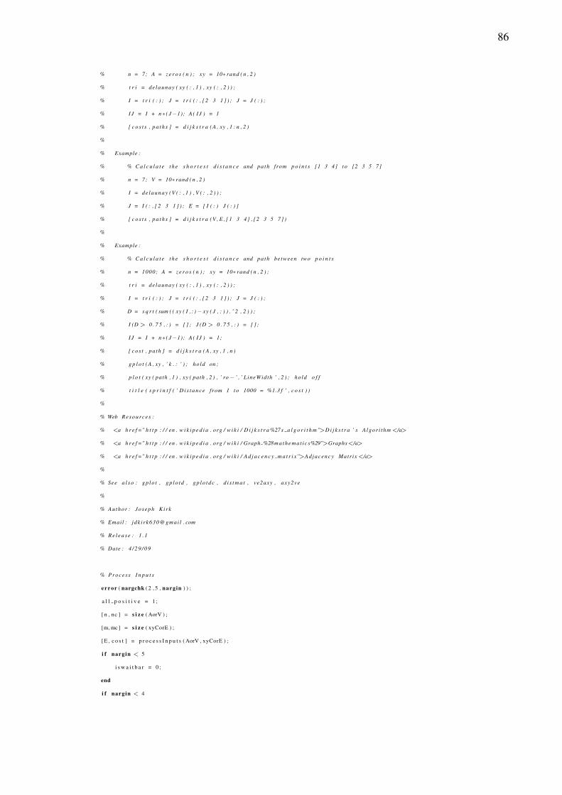
86
% n = 7; A = z e r o s ( n ) ; xy = 10∗ rand ( n , 2 )
% t r i = d e l a u n a y ( xy ( : , 1 ) , xy ( : , 2 ) ) ;
% I = t r i ( : ) ; J = t r i ( : , [ 2 3 1 ] ) ; J = J ( : ) ;
% I J = I + n ∗ ( J−1); A ( I J ) = 1
% [ c o s t s , p a t h s ] = d i j k s t r a ( A , xy , 1 : n , 2 )
%
% Example :
% % C a l c u l a t e t h e s h o r t e s t d i s t a n c e and pa th from p o i n t s [1 3 4] t o [2 3 5 7]
% n = 7; V = 10∗ rand ( n , 2 )
% I = d e l a u n a y ( V ( : , 1 ) , V ( : , 2 ) ) ;
% J = I ( : , [ 2 3 1 ] ) ; E = [ I ( : ) J ( : ) ]
% [ c o s t s , p a t h s ] = d i j k s t r a ( V , E , [ 1 3 4 ] , [ 2 3 5 7 ] )
%
% Example :
% % C a l c u l a t e t h e s h o r t e s t d i s t a n c e and pa th be tween two p o i n t s
% n = 1000; A = z e r o s ( n ) ; xy = 10∗ rand ( n , 2 ) ;
% t r i = d e l a u n a y ( xy ( : , 1 ) , xy ( : , 2 ) ) ;
% I = t r i ( : ) ; J = t r i ( : , [ 2 3 1 ] ) ; J = J ( : ) ;
% D = s q r t ( sum ( ( xy ( I , : ) − xy ( J , : ) ) . ˆ 2 , 2 ) ) ;
% I (D > 0 . 7 5 , : ) = [ ] ; J (D > 0 . 7 5 , : ) = [ ] ;
% I J = I + n ∗ ( J−1); A ( I J ) = 1;
% [ c o s t , pa th ] = d i j k s t r a ( A , xy , 1 , n )
% g p l o t ( A , xy , ’ k . : ’ ) ; ho ld on ;
% p l o t ( xy ( path , 1 ) , xy ( path , 2 ) , ’ ro − ’ , ’ L ineWidth ’ , 2 ) ; ho ld o f f
% t i t l e ( s p r i n t f ( ’ D i s t a n c e from 1 t o 1000 = %1.3 f ’ , c o s t ) )
%
% Web R e s o u r c e s :
% <a h r e f =” h t t p : / / en . w i k i p e d i a . org / w i k i / D i j k s t r a %27 s a l g o r i t h m”>D i j k s t r a ’ s A lgor i thm </a>
% <a h r e f =” h t t p : / / en . w i k i p e d i a . org / w i k i / Graph %28m a t h e m a t i c s%29”>Graphs</a>
% <a h r e f =” h t t p : / / en . w i k i p e d i a . org / w i k i / A d j a c e n c y m a t r i x”>Adjacency Matr ix </a>
%
% See a l s o : g p l o t , g p l o t d , g p l o t d c , d i s t m a t , ve2axy , axy2ve
%
% Author : Joseph Ki rk
% Email : j dk i r k630@gmai l . com
% R e l e a s e : 1 . 1
% Date : 4 / 2 9 / 0 9
% P r o c e s s I n p u t s
error ( nargchk ( 2 , 5 , nargin ) ) ;
a l l p o s i t i v e = 1 ;
[ n , nc ] = s i z e ( AorV ) ;
[m, mc ] = s i z e ( xyCorE ) ;
[ E , c o s t ] = p r o c e s s I n p u t s ( AorV , xyCorE ) ;
i f nargin < 5
i s w a i t b a r = 0 ;
end
i f nargin < 4
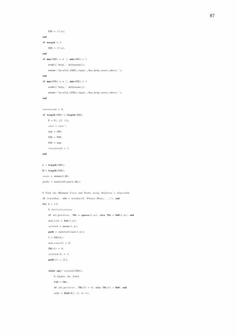
87
FID = ( 1 : n ) ;
end
i f nargin < 3
SID = ( 1 : n ) ;
end
i f max ( SID ) > n | | min ( SID ) < 1
e v a l ( [ ’ h e l p ’ mf i lename ] ) ;
error ( ’ I n v a l i d [ SID ] i n p u t . See h e l p n o t e s above . ’ ) ;
end
i f max ( FID ) > n | | min ( FID ) < 1
e v a l ( [ ’ h e l p ’ mf i lename ] ) ;
error ( ’ I n v a l i d [ FID ] i n p u t . See h e l p n o t e s above . ’ ) ;
end
i s r e v e r s e d = 0 ;
i f l e n g t h ( FID ) < l e n g t h ( SID )
E = E ( : , [ 2 1 ] ) ;
c o s t = c o s t ’ ;
tmp = SID ;
SID = FID ;
FID = tmp ;
i s r e v e r s e d = 1 ;
end
L = l e n g t h ( SID ) ;
M = l e n g t h ( FID ) ;
c o s t s = z e r o s ( L ,M) ;
p a t h s = num2ce l l ( nan ( L ,M) ) ;
% Find t h e Minimum C o s t s and Pa ths u s i n g D i j k s t r a ’ s A l g o r i t h m
i f i s w a i t b a r , wbh = w a i t b a r ( 0 , ’ P l e a s e Wait . . . ’ ) ; end
f o r k = 1 : L
% I n i t i a l i z a t i o n s
i f a l l p o s i t i v e , TBL = sp ar se ( 1 , n ) ; e l s e TBL = NaN ( 1 , n ) ; end
m i n c o s t = I n f ( 1 , n ) ;
s e t t l e d = z e r o s ( 1 , n ) ;
path = num2ce l l ( nan ( 1 , n ) ) ;
I = SID ( k ) ;
m i n c o s t ( I ) = 0 ;
TBL( I ) = 0 ;
s e t t l e d ( I ) = 1 ;
path ( I ) = { I } ;
whi le any ( ˜ s e t t l e d ( FID ) )
% Update t h e Tab le
TAB = TBL ;
i f a l l p o s i t i v e , TBL( I ) = 0 ; e l s e TBL( I ) = NaN ; end
n i d s = f i n d ( E ( : , 1 ) == I ) ;
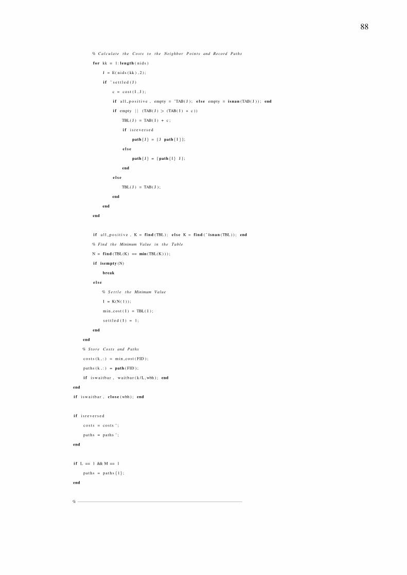
88
% C a l c u l a t e t h e C o s t s t o t h e Neighbor P o i n t s and Record Pa ths
f o r kk = 1 : l e n g t h ( n i d s )
J = E ( n i d s ( kk ) , 2 ) ;
i f ˜ s e t t l e d ( J )
c = c o s t ( I , J ) ;
i f a l l p o s i t i v e , empty = ˜TAB( J ) ; e l s e empty = i snan (TAB( J ) ) ; end
i f empty | | (TAB( J ) > (TAB( I ) + c ) )
TBL( J ) = TAB( I ) + c ;
i f i s r e v e r s e d
path{ J } = [ J path{ I } ] ;
e l s e
path{ J } = [ path{ I } J ] ;
end
e l s e
TBL( J ) = TAB( J ) ;
end
end
end
i f a l l p o s i t i v e , K = f i n d (TBL ) ; e l s e K = f i n d ( ˜ i snan (TBL ) ) ; end
% Find t h e Minimum Value i n t h e Tab le
N = f i n d (TBL(K) == min (TBL(K ) ) ) ;
i f i sempty (N)
break
e l s e
% S e t t l e t h e Minimum Value
I = K(N ( 1 ) ) ;
m i n c o s t ( I ) = TBL( I ) ;
s e t t l e d ( I ) = 1 ;
end
end
% S t o r e C o s t s and Pa ths
c o s t s ( k , : ) = m i n c o s t ( FID ) ;
p a t h s ( k , : ) = path ( FID ) ;
i f i s w a i t b a r , w a i t b a r ( k / L , wbh ) ; end
end
i f i s w a i t b a r , c l o s e ( wbh ) ; end
i f i s r e v e r s e d
c o s t s = c o s t s ’ ;
p a t h s = p a t h s ’ ;
end
i f L == 1 && M == 1
p a t h s = p a t h s {1} ;
end
% −−−−−−−−−−−−−−−−−−−−−−−−−−−−−−−−−−−−−−−−−−−−−−−−−−−−−−−−−−−−−−−−−−−
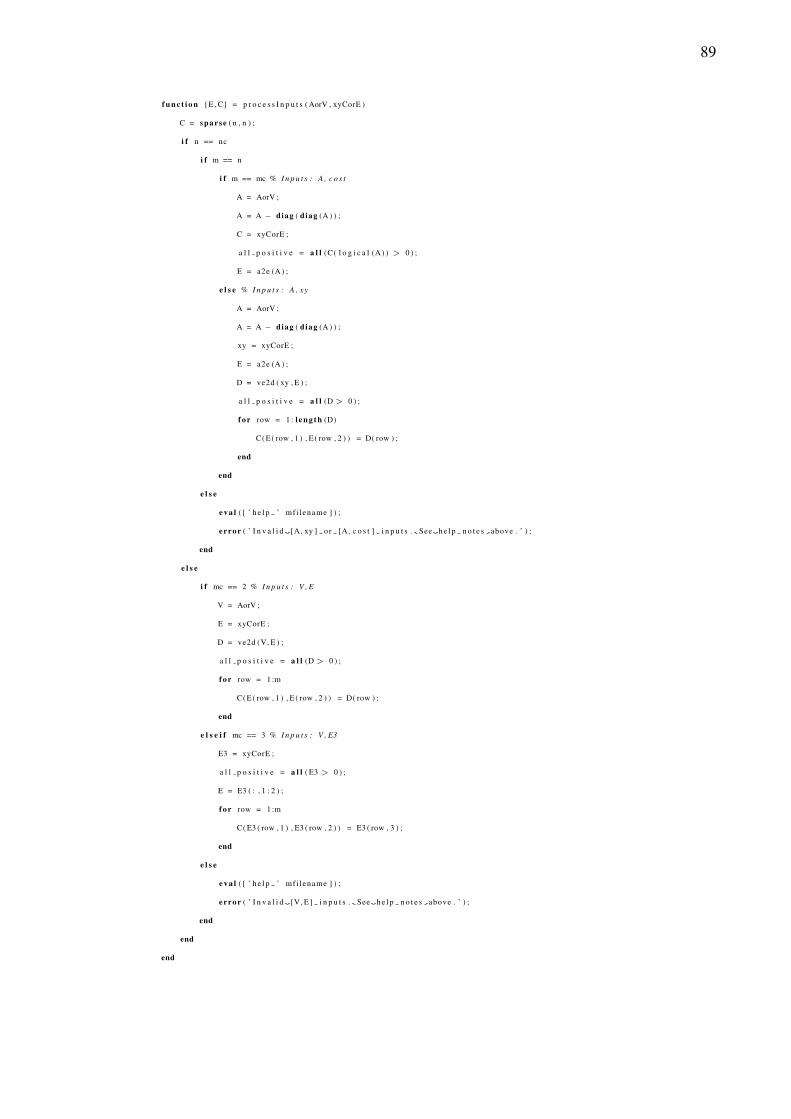
89
f u n c t i o n [ E , C] = p r o c e s s I n p u t s ( AorV , xyCorE )
C = sp ar se ( n , n ) ;
i f n == nc
i f m == n
i f m == mc % I n p u t s : A , c o s t
A = AorV ;
A = A − diag ( diag (A ) ) ;
C = xyCorE ;
a l l p o s i t i v e = a l l (C( l o g i c a l (A) ) > 0 ) ;
E = a2e (A ) ;
e l s e % I n p u t s : A , xy
A = AorV ;
A = A − diag ( diag (A ) ) ;
xy = xyCorE ;
E = a2e (A ) ;
D = ve2d ( xy , E ) ;
a l l p o s i t i v e = a l l (D > 0 ) ;
f o r row = 1 : l e n g t h (D)
C( E ( row , 1 ) , E ( row , 2 ) ) = D( row ) ;
end
end
e l s e
e v a l ( [ ’ h e l p ’ mf i lename ] ) ;
error ( ’ I n v a l i d [A, xy ] o r [A, c o s t ] i n p u t s . See h e l p n o t e s above . ’ ) ;
end
e l s e
i f mc == 2 % I n p u t s : V , E
V = AorV ;
E = xyCorE ;
D = ve2d (V, E ) ;
a l l p o s i t i v e = a l l (D > 0 ) ;
f o r row = 1 :m
C( E ( row , 1 ) , E ( row , 2 ) ) = D( row ) ;
end
e l s e i f mc == 3 % I n p u t s : V , E3
E3 = xyCorE ;
a l l p o s i t i v e = a l l ( E3 > 0 ) ;
E = E3 ( : , 1 : 2 ) ;
f o r row = 1 :m
C( E3 ( row , 1 ) , E3 ( row , 2 ) ) = E3 ( row , 3 ) ;
end
e l s e
e v a l ( [ ’ h e l p ’ mf i lename ] ) ;
error ( ’ I n v a l i d [V, E ] i n p u t s . See h e l p n o t e s above . ’ ) ;
end
end
end

90
% Conver t Ad jacency Ma t r i x t o Edge L i s t
f u n c t i o n E = a2e (A)
[ I , J ] = f i n d (A ) ;
E = [ I J ] ;
end
% Compute E u c l i d e a n D i s t a n c e f o r Edges
f u n c t i o n D = ve2d (V, E )
VI = V( E ( : , 1 ) , : ) ;
VJ = V( E ( : , 2 ) , : ) ;
D = s q r t ( sum ( ( VI − VJ ) . ˆ 2 , 2 ) ) ;
end
end
f u n c t i o n i d = g r e e d y f a r t h e s t a l g o r i t h m ( s e l f I D , conn , d s t i d , Node Pos )
% pass i n t h e d e s t i n a t i o n ID , and t h e row o f t h e p r e s e n t node
% i n t h e c o n n e c t i v i t y m a t r i x .
i d = 0 ;
C o n n q u i c k r e f = [ ] ;
f o r i =1 : l e n g t h ( conn )
i f i == s e l f I D ;
c o n t i n u e
end
i f conn ( i )
% i f t h e nodes are connec t ed ,
% s t o r e t h a t index , we ’ l l use i t l a t e r
C o n n q u i c k r e f = [ C o n n q u i c k r e f i ] ;
end
end
% we have a l i s t o f a l l nodes t h a t are c o n n e c t e d
% and we can r e f e r e n c e t h e i r p l a c e i n t h e p o s i t i o n m a t r i x
Pos = z e r o s ( l e n g t h ( C o n n q u i c k r e f ) + 1 , 1 ) ;
f o r i = 1 : ( l e n g t h ( C o n n q u i c k r e f ) )
% s t a r t i n g a t i n d e x 2 , go ing t o t h e end o f t h e q u i c k r e f
Pos ( i + 1 , : ) = Node Pos ( C o n n q u i c k r e f ( i ) , 1 ) ;
end
Pos ( 1 , : ) = Node Pos ( d s t i d , 1 ) ;
% we ’ ve b u i l t t h e a r r a y o f p o s i t i o n s , we need t o c a l c u l a t e d i s t a n c e
d i s t = s q u a r e f o r m ( p d i s t ( Pos ) ) ;
% t h i s i s a t ime−saver , b u t n o t a space−s a v e r .
% we can l o o k a t t h e f i r s t −column alone , d i s t ( 2 : l en , 1 ) , b a s i c a l l y
% d i s t ( 1 , 1 ) == 0 , by d e f i n i t i o n , i t ’ s t h e d i s t a n c e be tween t h e
% d e s t i n a t i o n and i t s e l f .
t m p d i s t a n c e = i n f ;
f o r i = 1 : l e n g t h ( d i s t ( : , 1 ) )
i f i == 1
c o n t i n u e
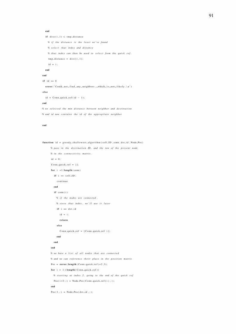
91
end
i f d i s t ( i , 1 ) < t m p d i s t a n c e
% i f t h e d i s t a n c e i s t h e l e a s t we ’ ve found
% s e l e c t t h a t i n d e x and d i s t a n c e
% t h a t i n d e x can t h e n be used t o s e l e c t from t h e q u i c k r e f .
t m p d i s t a n c e = d i s t ( i , 1 ) ;
i d = i ;
end
end
i f i d == 0
error ( ’ Could n o t f i n d any n e i g h b o r s , which i s n o t l i k e l y . \ n ’ )
e l s e
i d = C o n n q u i c k r e f ( i d − 1 ) ;
end
% we s e l e c t e d t h e min d i s t a n c e be tween n e i g h b o r and d e s t i n a t i o n
% and i d now c o n t a i n s t h e i d o f t h e a p p r o p r i a t e n e i g h b o r
end
f u n c t i o n i d = g r e e d y s h a l l o w e s t a l g o r i t h m ( s e l f I D , conn , d s t i d , Node Pos )
% pass i n t h e d e s t i n a t i o n ID , and t h e row o f t h e p r e s e n t node
% i n t h e c o n n e c t i v i t y m a t r i x .
i d = 0 ;
C o n n q u i c k r e f = [ ] ;
f o r i =1 : l e n g t h ( conn )
i f i == s e l f I D ;
c o n t i n u e
end
i f conn ( i )
% i f t h e nodes are connec t ed ,
% s t o r e t h a t index , we ’ l l use i t l a t e r
i f i == d s t i d
i d = i ;
re turn
e l s e
C o n n q u i c k r e f = [ C o n n q u i c k r e f i ] ;
end
end
end
% we have a l i s t o f a l l nodes t h a t are c o n n e c t e d
% and we can r e f e r e n c e t h e i r p l a c e i n t h e p o s i t i o n m a t r i x
Pos = z e r o s ( l e n g t h ( C o n n q u i c k r e f ) + 2 , 3 ) ;
f o r i = 1 : ( l e n g t h ( C o n n q u i c k r e f ) )
% s t a r t i n g a t i n d e x 2 , go ing t o t h e end o f t h e q u i c k r e f
Pos ( i + 2 , : ) = Node Pos ( C o n n q u i c k r e f ( i ) , : ) ;
end
Pos ( 1 , : ) = Node Pos ( d s t i d , : ) ;
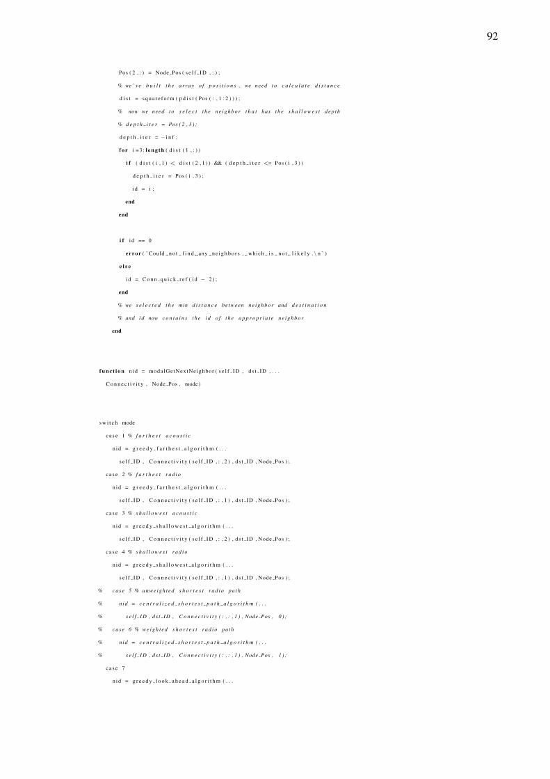
92
Pos ( 2 , : ) = Node Pos ( s e l f I D , : ) ;
% we ’ ve b u i l t t h e a r r a y o f p o s i t i o n s , we need t o c a l c u l a t e d i s t a n c e
d i s t = s q u a r e f o r m ( p d i s t ( Pos ( : , 1 : 2 ) ) ) ;
% now we need t o s e l e c t t h e n e i g h b o r t h a t has t h e s h a l l o w e s t d e p t h
% d e p t h i t e r = Pos ( 2 , 3 ) ;
d e p t h i t e r = − i n f ;
f o r i =3 : l e n g t h ( d i s t ( 1 , : ) )
i f ( d i s t ( i , 1 ) < d i s t ( 2 , 1 ) ) && ( d e p t h i t e r <= Pos ( i , 3 ) )
d e p t h i t e r = Pos ( i , 3 ) ;
i d = i ;
end
end
i f i d == 0
error ( ’ Could n o t f i n d any n e i g h b o r s , which i s n o t l i k e l y . \ n ’ )
e l s e
i d = C o n n q u i c k r e f ( i d − 2 ) ;
end
% we s e l e c t e d t h e min d i s t a n c e be tween n e i g h b o r and d e s t i n a t i o n
% and i d now c o n t a i n s t h e i d o f t h e a p p r o p r i a t e n e i g h b o r
end
f u n c t i o n n i d = modalGetNextNeighbor ( s e l f I D , d s t I D , . . .
C o n n e c t i v i t y , Node Pos , mode )
s w i t c h mode
c a s e 1 % f a r t h e s t a c o u s t i c
n i d = g r e e d y f a r t h e s t a l g o r i t h m ( . . .
s e l f I D , C o n n e c t i v i t y ( s e l f I D , : , 2 ) , d s t I D , Node Pos ) ;
c a s e 2 % f a r t h e s t r a d i o
n i d = g r e e d y f a r t h e s t a l g o r i t h m ( . . .
s e l f I D , C o n n e c t i v i t y ( s e l f I D , : , 1 ) , d s t I D , Node Pos ) ;
c a s e 3 % s h a l l o w e s t a c o u s t i c
n i d = g r e e d y s h a l l o w e s t a l g o r i t h m ( . . .
s e l f I D , C o n n e c t i v i t y ( s e l f I D , : , 2 ) , d s t I D , Node Pos ) ;
c a s e 4 % s h a l l o w e s t r a d i o
n i d = g r e e d y s h a l l o w e s t a l g o r i t h m ( . . .
s e l f I D , C o n n e c t i v i t y ( s e l f I D , : , 1 ) , d s t I D , Node Pos ) ;
% case 5 % u n w e i g h t e d s h o r t e s t r a d i o pa th
% n i d = c e n t r a l i z e d s h o r t e s t p a t h a l g o r i t h m ( . . .
% s e l f I D , d s t I D , C o n n e c t i v i t y ( : , : , 1 ) , Node Pos , 0 ) ;
% case 6 % w e i g h t e d s h o r t e s t r a d i o pa th
% n i d = c e n t r a l i z e d s h o r t e s t p a t h a l g o r i t h m ( . . .
% s e l f I D , d s t I D , C o n n e c t i v i t y ( : , : , 1 ) , Node Pos , 1 ) ;
c a s e 7
n i d = g r e e d y l o o k a h e a d a l g o r i t h m ( . . .
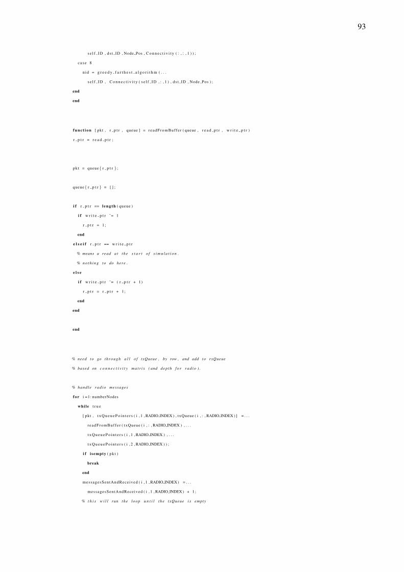
93
s e l f I D , d s t I D , Node Pos , C o n n e c t i v i t y ( : , : , 1 ) ) ;
c a s e 8
n i d = g r e e d y f a r t h e s t a l g o r i t h m ( . . .
s e l f I D , C o n n e c t i v i t y ( s e l f I D , : , 1 ) , d s t I D , Node Pos ) ;
end
end
f u n c t i o n [ pkt , r p t r , queue ] = r e a d F r o m B u f f e r ( queue , r e a d p t r , w r i t e p t r )
r p t r = r e a d p t r ;
p k t = queue { r p t r } ;
queue { r p t r } = [ ] ;
i f r p t r == l e n g t h ( queue )
i f w r i t e p t r ˜= 1
r p t r = 1 ;
end
e l s e i f r p t r == w r i t e p t r
% means a read a t t h e s t a r t o f s i m u l a t i o n .
% n o t h i n g t o do here .
e l s e
i f w r i t e p t r ˜= ( r p t r + 1 )
r p t r = r p t r + 1 ;
end
end
end
% need t o go t h r o u g h a l l o f txQueue , by row , and add t o rxQueue
% based on c o n n e c t i v i t y m a t r i x ( and d e p t h f o r r a d i o ) .
% ha nd le r a d i o messages
f o r i =1 : numberNodes
whi le t r u e
[ pkt , t x Q u e u e P o i n t e r s ( i , 1 , RADIO INDEX ) , txQueue ( i , : , RADIO INDEX ) ] = . . .
r e a d F r o m B u f f e r ( txQueue ( i , : , RADIO INDEX ) , . . .
t x Q u e u e P o i n t e r s ( i , 1 , RADIO INDEX ) , . . .
t x Q u e u e P o i n t e r s ( i , 2 , RADIO INDEX ) ) ;
i f i sempty ( p k t )
break
end
messagesSen tAndRece ived ( i , 1 , RADIO INDEX ) = . . .
messagesSen tAndRece ived ( i , 1 , RADIO INDEX ) + 1 ;
% t h i s w i l l run t h e loop u n t i l t h e txQueue i s empty
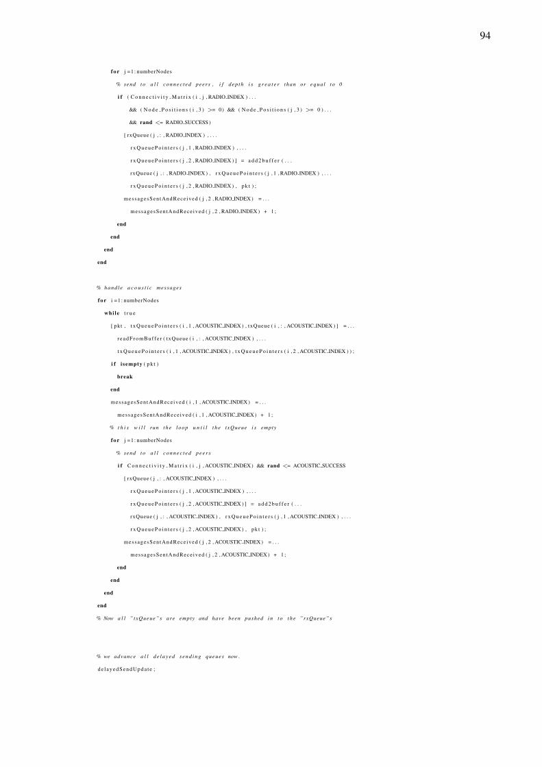
94
f o r j =1 : numberNodes
% send t o a l l c o n n e c t e d peers , i f d e p t h i s g r e a t e r than or e q u a l t o 0
i f ( C o n n e c t i v i t y M a t r i x ( i , j , RADIO INDEX ) . . .
&& ( N o d e P o s i t i o n s ( i , 3 ) >= 0) && ( N o d e P o s i t i o n s ( j , 3 ) >= 0 ) . . .
&& rand <= RADIO SUCCESS )
[ rxQueue ( j , : , RADIO INDEX ) , . . .
r x Q u e u e P o i n t e r s ( j , 1 , RADIO INDEX ) , . . .
r x Q u e u e P o i n t e r s ( j , 2 , RADIO INDEX ) ] = a d d 2 b u f f e r ( . . .
rxQueue ( j , : , RADIO INDEX ) , r x Q u e u e P o i n t e r s ( j , 1 , RADIO INDEX ) , . . .
r x Q u e u e P o i n t e r s ( j , 2 , RADIO INDEX ) , p k t ) ;
messagesSen tAndRece ived ( j , 2 , RADIO INDEX ) = . . .
messagesSen tAndRece ived ( j , 2 , RADIO INDEX ) + 1 ;
end
end
end
end
% ha nd le a c o u s t i c messages
f o r i =1 : numberNodes
whi le t r u e
[ pkt , t x Q u e u e P o i n t e r s ( i , 1 , ACOUSTIC INDEX ) , txQueue ( i , : , ACOUSTIC INDEX ) ] = . . .
r e a d F r o m B u f f e r ( txQueue ( i , : , ACOUSTIC INDEX ) , . . .
t x Q u e u e P o i n t e r s ( i , 1 , ACOUSTIC INDEX ) , t x Q u e u e P o i n t e r s ( i , 2 , ACOUSTIC INDEX ) ) ;
i f i sempty ( p k t )
break
end
messagesSen tAndRece ived ( i , 1 , ACOUSTIC INDEX ) = . . .
messagesSen tAndRece ived ( i , 1 , ACOUSTIC INDEX ) + 1 ;
% t h i s w i l l run t h e loop u n t i l t h e txQueue i s empty
f o r j =1 : numberNodes
% send t o a l l c o n n e c t e d p e e r s
i f C o n n e c t i v i t y M a t r i x ( i , j , ACOUSTIC INDEX ) && rand <= ACOUSTIC SUCCESS
[ rxQueue ( j , : , ACOUSTIC INDEX ) , . . .
r x Q u e u e P o i n t e r s ( j , 1 , ACOUSTIC INDEX ) , . . .
r x Q u e u e P o i n t e r s ( j , 2 , ACOUSTIC INDEX ) ] = a d d 2 b u f f e r ( . . .
rxQueue ( j , : , ACOUSTIC INDEX ) , r x Q u e u e P o i n t e r s ( j , 1 , ACOUSTIC INDEX ) , . . .
r x Q u e u e P o i n t e r s ( j , 2 , ACOUSTIC INDEX ) , p k t ) ;
messagesSen tAndRece ived ( j , 2 , ACOUSTIC INDEX ) = . . .
messagesSen tAndRece ived ( j , 2 , ACOUSTIC INDEX ) + 1 ;
end
end
end
end
% Now a l l ” txQueue ” s are empty and have been pushed i n t o t h e ”rxQueue” s
% we advance a l l d e l a y e d s e n d i n g queues now .
de layedSendUpda te ;
95
UW Sim Setup ;
Sim Run ;
% [ e n d p o s i t i o n s , s e n t A n d R e c e i v e d , energyUsed , t i m e E l a p s e d ] = . . .
% UW Sim Run ( N o d e P o s i t i o n s , C o n n e c t i v i t y M a t r i x , txQueue , rxQueue , . . .
% txQueuePtr , rxQueuePtr , mode , P ac k e t ) ;
%
% g r a p h r e s u l t s ;
%t o c
c o n s t a n t I n i t ;
t o p o l o g y I n i t ;
c o n n e c t i v i t y C r e a t e ;
d e l a y e d S e n d I n i t ;
CommInit ;