1 signals and systems - kauno technologijos …girrol/skaidres/literatura/angliska/pateiktys/... ·...

1

1 Signals and Systems

introducing “language for describing signals and systems”

Outline

1.1 Continuous–Time and Discrete–Time Signals

1.2 Elementary Signals

1.3 Continuous–Time and Discrete–Time Systems

1.4 Basic System Properties

Lampe, Schober: Signals and Communications

2

1.1 Continuous–Time and Discrete–Time Signals

� Unified representation of physical phenomena by signals

Signal: Function or sequence that represents information.

– One or more independent variables

– Continuous or discrete independent variables

– Examples: time, location, etc.

1.1.1 Mathematical Representation

� Continuous–time signals

– Symbol t for independent variable

– Use parentheses (·)

Continuous–time signal: x(t)

– Graphical representation

0 t

x(t)


3

� Discrete–time signals

– Symbol n for independent variable

– Use brackets [·]

Discrete–time signal: x[n]

– Graphical representation

x[0]

x[1]x[−1]

0 321

x[2]x[−2]

n−3 −2 −1

54

x[n]


4

1.1.2 Signal Energy and Power

� Often classification of signals according to energy and power

– Terminology energy and power used for any signal x(t), x[n]

– Need not necessarily have a physical meaning

� Signal energy

– Energy of a possibly complex continuous–time signal x(t) in

interval t1 ≤ t ≤ t2

E(t1, t2) =

t2∫

t1

|x(t)|2 dt

– Energy of a possibly complex discrete–time signal x[n] in interval

n1 ≤ n ≤ n2

E(n1, n2) =

n2∑

n=n1

|x[n]|2

– Total energy

E∞ = E(−∞,∞) =

∞∫

−∞

|x(t)|2 dt

E∞ = E(−∞,∞) =

∞∑

n=−∞

|x[n]|2


5

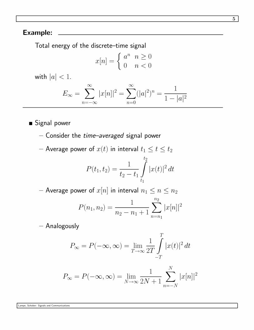
Example:

Total energy of the discrete–time signal

x[n] =

{

an n ≥ 0

0 n < 0

with |a| < 1.

E∞ =

∞∑

n=−∞

|x[n]|2 =

∞∑

n=0

(|a|2)n =1

1 − |a|2

� Signal power

– Consider the time–averaged signal power

– Average power of x(t) in interval t1 ≤ t ≤ t2

P (t1, t2) =1

t2 − t1

t2∫

t1

|x(t)|2 dt

– Average power of x[n] in interval n1 ≤ n ≤ n2

P (n1, n2) =1

n2 − n1 + 1

n2∑

n=n1

|x[n]|2

– Analogously

P∞ = P (−∞,∞) = limT→∞

1

2T

T∫

−T

|x(t)|2 dt

P∞ = P (−∞,∞) = limN→∞

1

2N + 1

N∑

n=−N

|x[n]|2


6

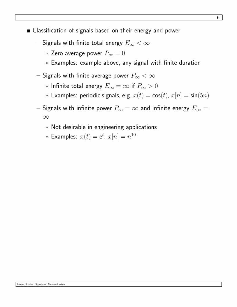
� Classification of signals based on their energy and power

– Signals with finite total energy E∞ < ∞

∗ Zero average power P∞ = 0

∗ Examples: example above, any signal with finite duration

– Signals with finite average power P∞ < ∞

∗ Infinite total energy E∞ = ∞ if P∞ > 0

∗ Examples: periodic signals, e.g. x(t) = cos(t), x[n] = sin(5n)

– Signals with infinite power P∞ = ∞ and infinite energy E∞ =

∞

∗ Not desirable in engineering applications

∗ Examples: x(t) = et, x[n] = n10


7

1.1.3 Transformations of the Independent Variable

� Time shift

– Replace t → t − t0 x(t) → x(t − t0)

n → n − n0⇒ x[n] → x[n − n0]

– Delay: t0, n0 > 0, Advance: t0, n0 < 0

� Time reversal

– Replace t → −t x(t) → x(−t)

n → −n ⇒ x[n] → x[−n]

� Time scaling

– Replace t → αt , α ∈ IR x(t) → x(αt)

n → αn , α ∈ ZZ ⇒ x[n] → x[αn]

– Continuous–time case: |α| < 1 : signal is linearly stretched

|α| > 1 : signal is linearly compressed

� Time shift, time reversal, and time scaling operations arise naturally

in the processing of signals


8

Example:

n

nt

n

n

t

t

Time-scaled signals

Time-reversed signals

Time-shifted signals

Signals

t

x[2n]

x[−n]

x[n − 4]

x(2/3t)

x(−t)

x(t − t0)

x(t) x[n]

t0


9

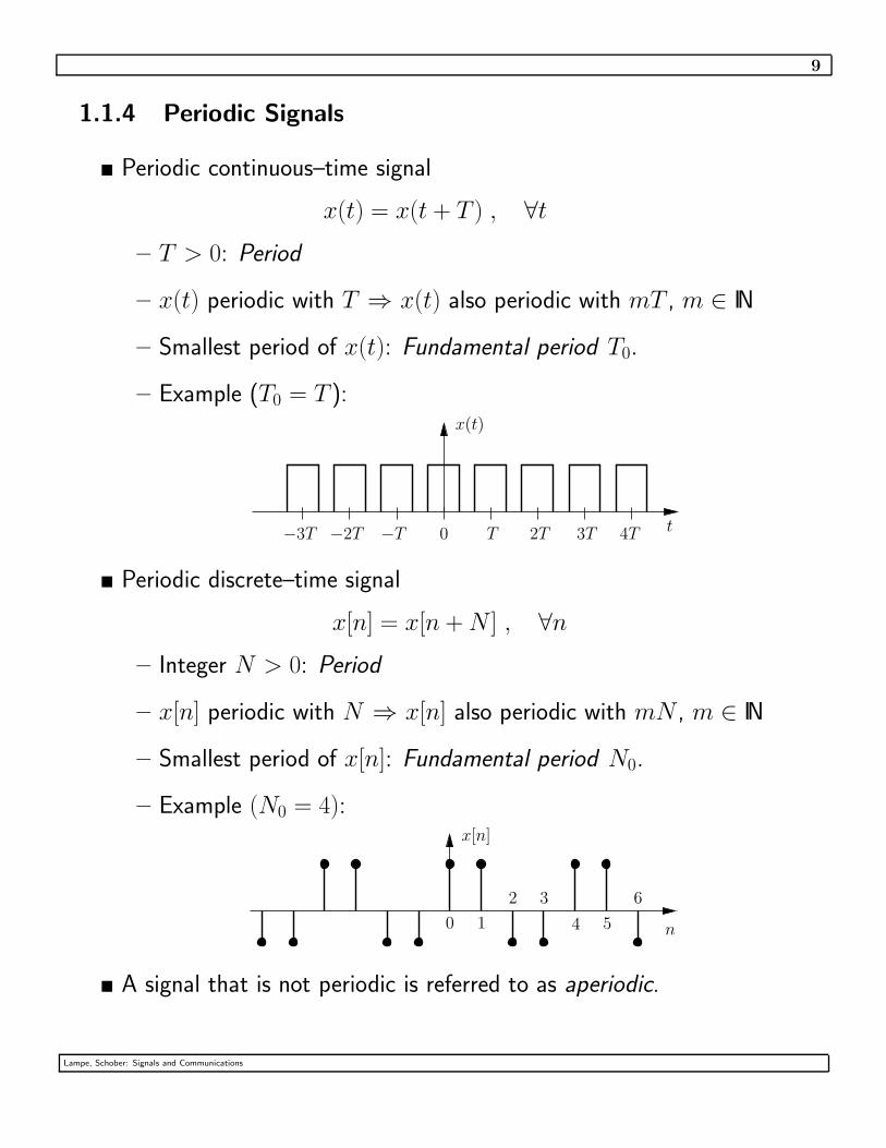
1.1.4 Periodic Signals

� Periodic continuous–time signal

x(t) = x(t + T ) , ∀t

– T > 0: Period

– x(t) periodic with T ⇒ x(t) also periodic with mT , m ∈ IN

– Smallest period of x(t): Fundamental period T0.

– Example (T0 = T ):

0

x(t)

t4T3T2T−3T −2T −T T

� Periodic discrete–time signal

x[n] = x[n + N ] , ∀n

– Integer N > 0: Period

– x[n] periodic with N ⇒ x[n] also periodic with mN , m ∈ IN

– Smallest period of x[n]: Fundamental period N0.

– Example (N0 = 4):

n

3 6

x[n]

0 1

2

54

� A signal that is not periodic is referred to as aperiodic.


10

1.1.5 Even and Odd Signals

� Even signal

x(−t) = x(t) or x[−n] = x[n]

– Example:x(t)

t

� Odd signal

x(−t) = −x(t) or x[−n] = −x[n]

– Example:

n

x[n]

– Necessarily: x(0) = 0 or x[0] = 0

� Decomposition of any signal into an even and odd part:

x(t) = Ev{x(t)} + Od{x(t)} or x[n] = Ev{x[n]} + Od{x[n]}

with

Ev{x(t)} =1

2(x(t) + x(−t)) or Ev{x[n]} =

1

2(x[n] + x[−n])

and

Od{x(t)} =1

2(x(t) − x(−t)) or Od{x[n]} =

1

2(x[n] − x[−n])


11

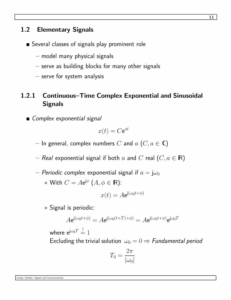
1.2 Elementary Signals

� Several classes of signals play prominent role

– model many physical signals

– serve as building blocks for many other signals

– serve for system analysis

1.2.1 Continuous–Time Complex Exponential and Sinusoidal

Signals

� Complex exponential signal

x(t) = Ceat

– In general, complex numbers C and a (C, a ∈ C)

– Real exponential signal if both a and C real (C, a ∈ IR)

– Periodic complex exponential signal if a = jω0

∗ With C = Aejφ (A, φ ∈ IR):

x(t) = Aej(ω0t+φ)

∗ Signal is periodic:

Aej(ω0t+φ) = Aej(ω0(t+T )+φ) = Aej(ω0t+φ)ejω0T

where ejω0T != 1

Excluding the trivial solution ω0 = 0 ⇒ Fundamental period

T0 =2π

|ω0|


12

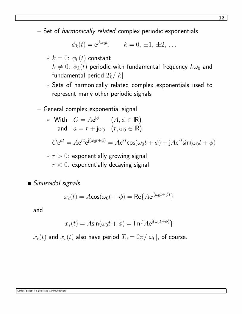
– Set of harmonically related complex periodic exponentials

φk(t) = ejkω0t, k = 0, ±1, ±2, . . .

∗ k = 0: φ0(t) constant

k 6= 0: φk(t) periodic with fundamental frequency kω0 and

fundamental period T0/|k|

∗ Sets of harmonically related complex exponentials used to

represent many other periodic signals

– General complex exponential signal

∗ With C = Aejφ (A, φ ∈ IR)

and a = r + jω0 (r, ω0 ∈ IR)

Ceat = Aertej(ω0t+φ) = Aertcos(ω0t + φ) + jAertsin(ω0t + φ)

∗ r > 0: exponentially growing signal

r < 0: exponentially decaying signal

� Sinusoidal signals

xc(t) = Acos(ω0t + φ) = Re{Aej(ω0t+φ)}

and

xs(t) = Asin(ω0t + φ) = Im{Aej(ω0t+φ)}

xc(t) and xs(t) also have period T0 = 2π/|ω0|, of course.


13

� Periodic signals have infinite total energy but finite average power.

– Exponential x(t) = ejω0t

∗ Energy over one period T0

Eperiod =

T0∫

0

|ejω0t|2 dt = T0

∗ Average power per period

Pperiod =Eperiod

T0= 1

∗ Average power

P∞ = limT→∞

1

2T

T∫

−T

|ejω0t|2 dt = 1


14

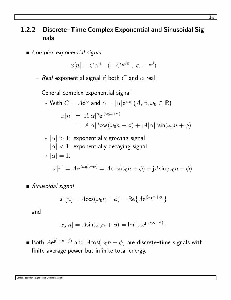
1.2.2 Discrete–Time Complex Exponential and Sinusoidal Sig-

nals

� Complex exponential signal

x[n] = Cαn (= Ceβn , α = eβ)

– Real exponential signal if both C and α real

– General complex exponential signal

∗ With C = Aejφ and α = |α|ejω0 (A, φ, ω0 ∈ IR)

x[n] = A|α|nej(ω0n+φ)

= A|α|ncos(ω0n + φ) + jA|α|nsin(ω0n + φ)

∗ |α| > 1: exponentially growing signal

|α| < 1: exponentially decaying signal

∗ |α| = 1:

x[n] = Aej(ω0n+φ) = Acos(ω0n + φ) + jAsin(ω0n + φ)

� Sinusoidal signal

xc[n] = Acos(ω0n + φ) = Re{Aej(ω0n+φ)}

and

xs[n] = Asin(ω0n + φ) = Im{Aej(ω0n+φ)}

� Both Aej(ω0n+φ) and Acos(ω0n + φ) are discrete–time signals with

finite average power but infinite total energy.


15

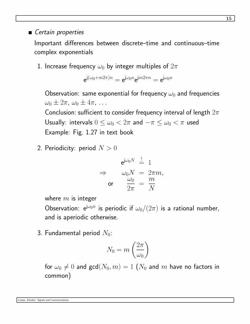
� Certain properties

Important differences between discrete–time and continuous–time

complex exponentials

1. Increase frequency ω0 by integer multiples of 2π

ej(ω0+m2π)n = ejω0nejm2πn = ejω0n

Observation: same exponential for frequency ω0 and frequencies

ω0 ± 2π, ω0 ± 4π, . . .

Conclusion: sufficient to consider frequency interval of length 2π

Usually: intervals 0 ≤ ω0 < 2π and −π ≤ ω0 < π used

Example: Fig. 1.27 in text book

2. Periodicity: period N > 0

ejω0N != 1

⇒ ω0N = 2πm,

orω0

2π=

m

N

where m is integer

Observation: ejω0n is periodic if ω0/(2π) is a rational number,

and is aperiodic otherwise.

3. Fundamental period N0:

N0 = m

(

2π

ω0

)

for ω0 6= 0 and gcd(N0, m) = 1 (N0 and m have no factors in

common)


16

Example:

– x(t) = cos(8πt/31)

ω0 =

Fundamental period T0 = 2π/ω0 =

– x[n] = cos(8πn/31) (= x(t = n))

ω0 =

Periodic?

Fundamental period N0 = m(2π/ω0) =

for m =

– x[n] = cos(n/6)

ω0 =

Periodic?

Fundamental period N0 = m(2π/ω0) =

for m =

� Set of harmonically related discrete–time periodic exponentials

φk[n] = ejk(2π/N)n, k = 0, ±1, . . .

– Common period N

– Observation:

φk+N [n] = ej(k+N)(2π/N)n = ejk(2π/N)nej2πn = φk[n]

⇒ Only N distinct complex exponentials φ0[n], φ1[n], . . .,

φN−1[n].


17

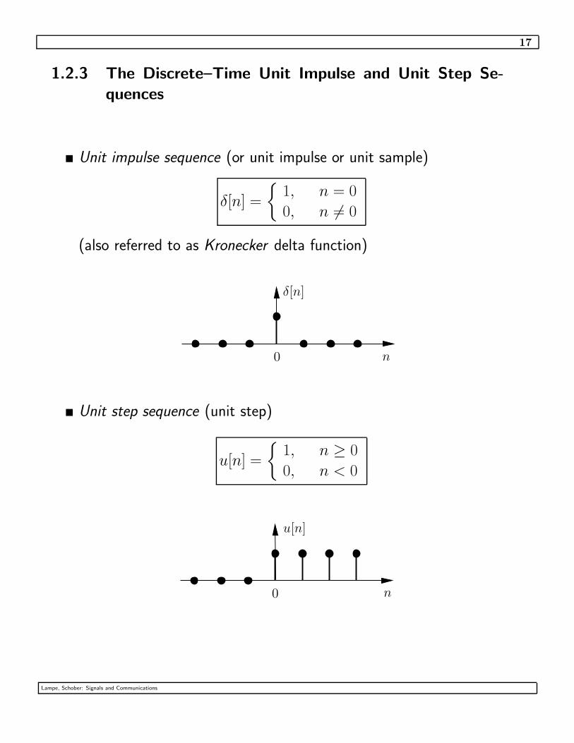
1.2.3 The Discrete–Time Unit Impulse and Unit Step Se-

quences

� Unit impulse sequence (or unit impulse or unit sample)

δ[n] =

{

1, n = 0

0, n 6= 0

(also referred to as Kronecker delta function)

n

δ[n]

0

� Unit step sequence (unit step)

u[n] =

{

1, n ≥ 0

0, n < 0

0 n

u[n]


18

� Relation between δ[n] and u[n]

– First order difference

δ[n] = u[n] − u[n − 1]

– Running sum

u[n] =n

∑

m=−∞

δ[m]

� Sampling property of unit impulse

x[n]δ[n − n0] = x[n0]δ[n − n0]

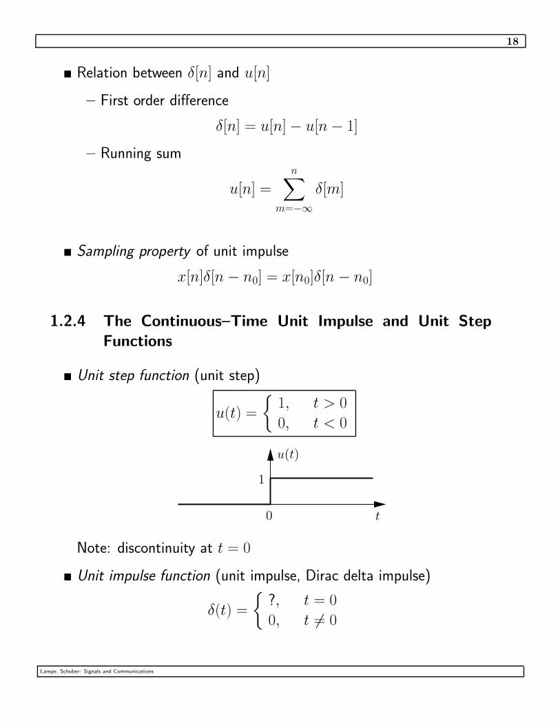
1.2.4 The Continuous–Time Unit Impulse and Unit Step

Functions

� Unit step function (unit step)

u(t) =

{

1, t > 0

0, t < 0

u(t)

t0

1

Note: discontinuity at t = 0

� Unit impulse function (unit impulse, Dirac delta impulse)

δ(t) =

{

?, t = 0

0, t 6= 0


19

Remark:

We use the short-hand notation:dx(t)

dt= x(t)

� Relation between δ(t) and u(t)

– First order derivative

δ(t) = u(t)

– Running integral

u(t) =

t∫

−∞

δ(τ ) dτ

Formal difficulty: u(t) is not differentiable in the conventional sense

because of its discontinuity at t = 0.

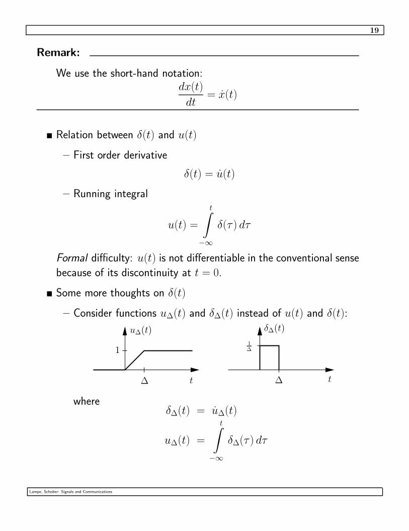
� Some more thoughts on δ(t)

– Consider functions u∆(t) and δ∆(t) instead of u(t) and δ(t):

u∆(t)

∆ t

δ∆(t)

1

∆

t∆

1

whereδ∆(t) = u∆(t)

u∆(t) =

t∫

−∞

δ∆(τ ) dτ


20

– Limit ∆ → 0

∗ u(t) = lim∆→0

u∆(t)

∗ δ(t) :

t

δ∆1(t)

δ∆3(t)

δ∆2(t)

∆3 ∆2 ∆1

1

∆1

1

∆3

1

∆2

Observe: Area under δ∆(t) always 1

⇒ δ(t) is an infinitesimally narrow impulse with area 1.

δ(t) = lim∆→0

δ∆(t)∞

∫

−∞

δ(τ ) dτ = 1

– Representation

a

t

aδ(t)

t0

1

t

δ(t − t0)

1

t

δ(t)


21

– Properties

∗ Sampling property (x(t) continuous at t = t0)

∞∫

−∞

x(τ )δ(τ − t0) dτ = x(t0)

x(t)δ(t − t0) = x(t0)δ(t − t0)

∗ Linearity

∞∫

−∞

(aδ(τ ) + bδ(τ ))x(τ ) dτ =

∞∫

−∞

aδ(τ )x(τ ) dτ +

∞∫

−∞

bδ(τ )x(τ ) dτ

= (a + b)x(0)

aδ(t) + bδ(t) = (a + b)δ(t)

∗ Time scaling (a ∈ IR)

∞∫

−∞

δ(aτ )x(τ ) dτ =

∞∫

−∞

1

|a|δ(ν)x(ν/a) dν =

1

|a|x(0)

δ(at) =1

|a|δ(t)


22

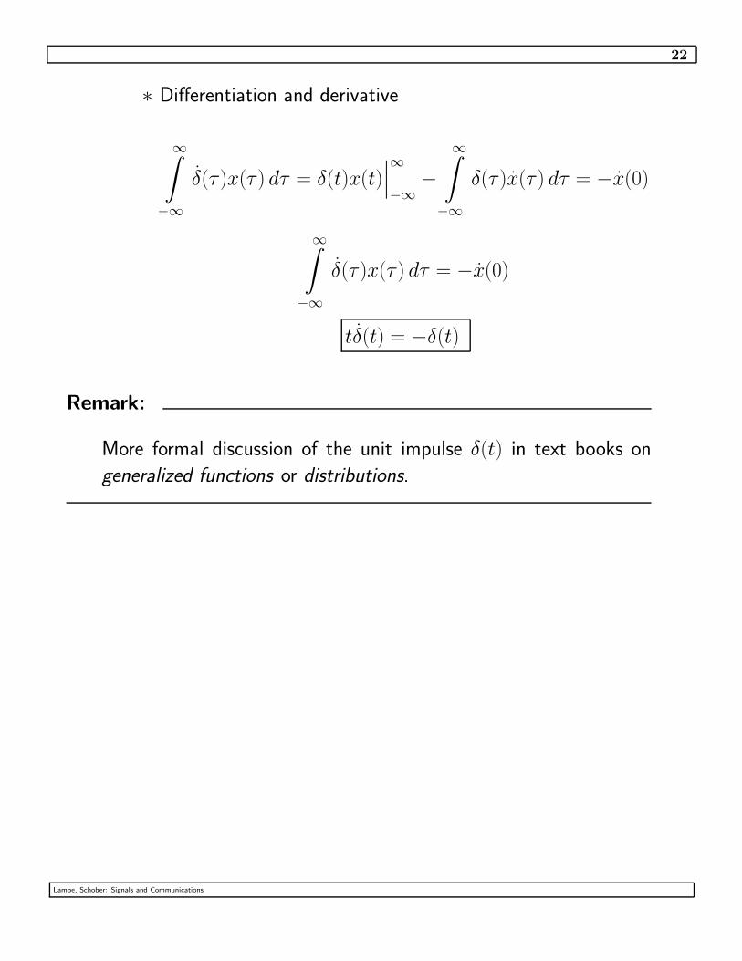
∗ Differentiation and derivative

∞∫

−∞

δ(τ )x(τ ) dτ = δ(t)x(t)∣

∣

∣

∞

−∞−

∞∫

−∞

δ(τ )x(τ ) dτ = −x(0)

∞∫

−∞

δ(τ )x(τ ) dτ = −x(0)

tδ(t) = −δ(t)

Remark:

More formal discussion of the unit impulse δ(t) in text books on

generalized functions or distributions.


23

1.3 Continuous–Time and Discrete–Time Systems

� Unified representation of physical processes by systems

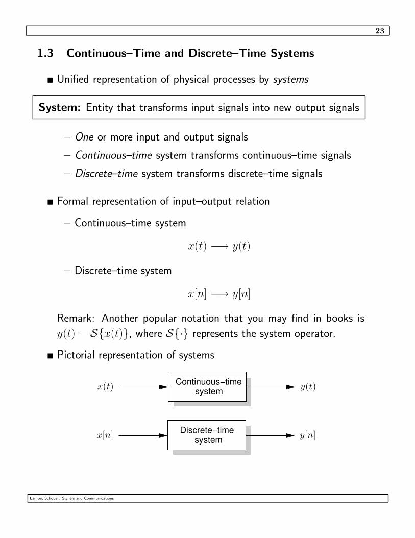
System: Entity that transforms input signals into new output signals

– One or more input and output signals

– Continuous–time system transforms continuous–time signals

– Discrete–time system transforms discrete–time signals

� Formal representation of input–output relation

– Continuous–time system

x(t) −→ y(t)

– Discrete–time system

x[n] −→ y[n]

Remark: Another popular notation that you may find in books is

y(t) = S{x(t)}, where S{·} represents the system operator.

� Pictorial representation of systems

Continuous−timesystem

x(t) y(t)

systemDiscrete−time

x[n] y[n]


24

1.3.1 Simple Examples of Systems

� Quadratic system

y(t) = (x(t))2

� System represented by a first order differential equation

y(t) + ay(t) = bx(t)

with constants a and b

� Delay system

y[n] = x[n − 1]

� System described by a first order difference equation

y[n] = ay[n − 1] + bx[n]

with constants a and b

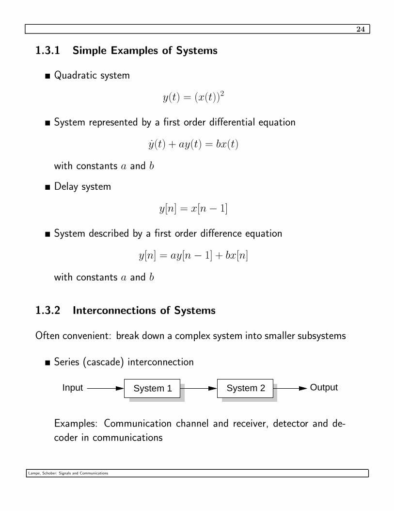
1.3.2 Interconnections of Systems

Often convenient: break down a complex system into smaller subsystems

� Series (cascade) interconnection

System 1 System 2Input Output

Examples: Communication channel and receiver, detector and de-

coder in communications


25

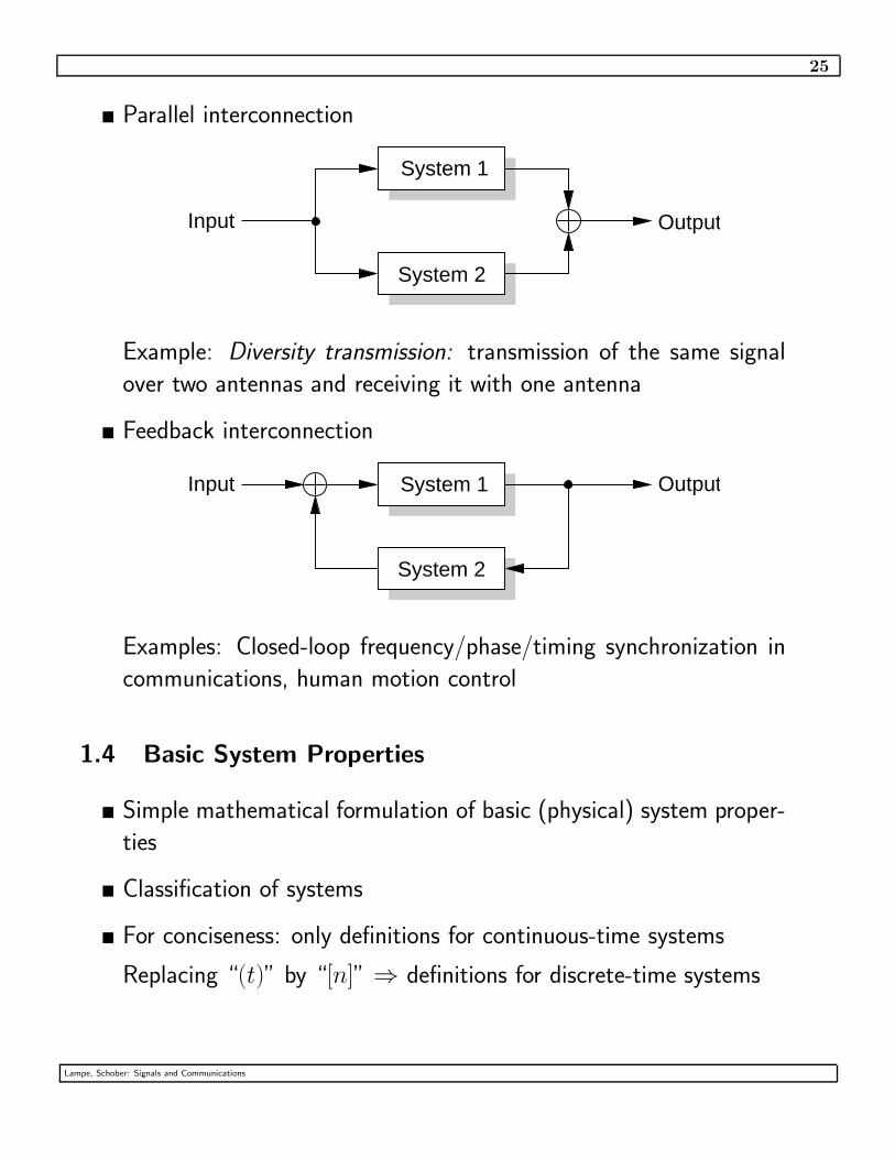
� Parallel interconnection

System 1

System 2

OutputInput

Example: Diversity transmission: transmission of the same signal

over two antennas and receiving it with one antenna

� Feedback interconnection

OutputInput

System 2

System 1

Examples: Closed-loop frequency/phase/timing synchronization in

communications, human motion control

1.4 Basic System Properties

� Simple mathematical formulation of basic (physical) system proper-

ties

� Classification of systems

� For conciseness: only definitions for continuous-time systems

Replacing “(t)” by “[n]” ⇒ definitions for discrete-time systems


26

1.4.1 Linearity

� Let x1(t) −→ y1(t) and x2(t) −→ y2(t)

Linear system if

1. Additivity

x1(t) + x2(t) −→ y1(t) + y2(t)

2. Homogeneity

ax1(t) −→ ay1(t) , ∀a ∈ C

� Linear systems possess property of superposition

Let xk(t) −→ yk(t), then

K∑

k=1

akxk(t) = x(t) −→ y(t) =K

∑

k=1

akyk(t)

� “Not linear” systems are referred to as nonlinear.

Example:

1. System y(t) = tx(t) is linear.

To see this let

x1(t) −→ y1(t) = tx1(t)

x2(t) −→ y2(t) = tx2(t)

and

x3(t) = ax1(t) + bx2(t) ,


27

and check

y3(t) = tx3(t) = tax1(t) + tbx2(t) = ay1(t) + by2(t) ,

i.e.,

ax1(t) + bx2(t) −→ ay1(t) + by2(t)

2. System y[n] = (x[n])2 is nonlinear.

To see this let

x1[n] −→ y1[n] = (x1[n])2

x2[n] −→ y2[n] = (x2[n])2

and check additivity for input x3[n] = x1[n] + x2[n]

y3[n] = (x3[n])2 = y1[n] + y2[n] + 2x1[n]x2[n]

6= y1[n] + y2[n]

3. System y(t) = (x(t))∗ is ?

1.4.2 Time Invariance

� Time invariant system if behavior and characteristics are time-invariant,

i.e., identical response to same input signal no matter when input

signal is applied

x(t − t0) −→ y(t − t0)

Example:

1. The system y(t) = (x(t))2 is ?

2. The system y[n] = nx[n] is ?


28

Remark:

Linear and time-invariant (linear time-invariant (LTI)) systems play

a prominent role for system modeling and analysis. The importance

of complex exponentials derives from the fact that they are eigen-

functions of LTI systems.

1.4.3 Systems with and without Memory

� Memoryless system if output signal depends only on present value

of input signal

� Otherwise, a system is said to possess memory or to be dispersive.

Example:

– Memoryless systems

1. Limiter: y[n] =

x[n] , −A ≤ x[n] ≤ A

−A , x[n] < −A

A , x[n] > A

2. Amplifier: y(t) = Ax(t)

– Systems with memory

1. Accumulator: y[n] =

n∑

k=−∞

x[k] = x[n] + y[n − 1]

2. Delay: y(t) = x(t − t0)

3. Capacitor: y(t) =1

C

t∫

−∞

x(τ ) dτ


29

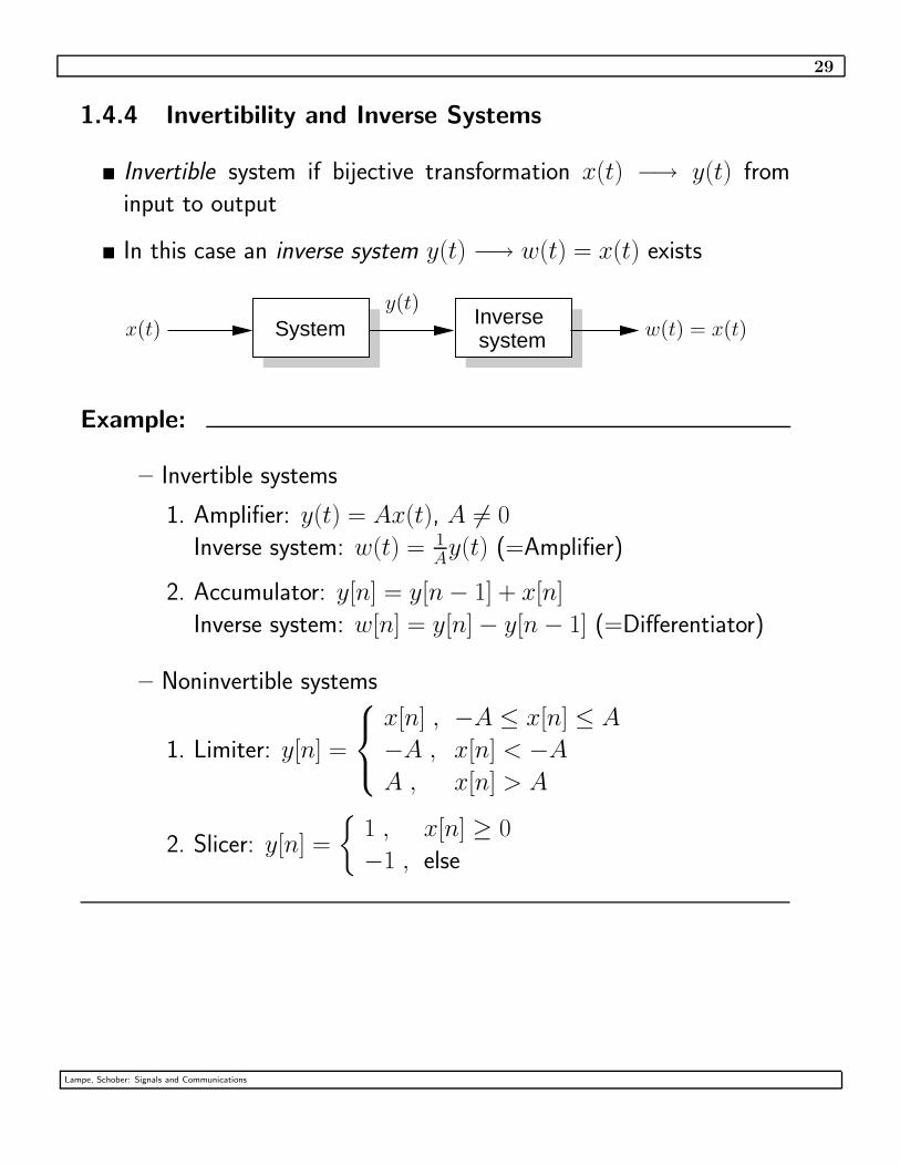
1.4.4 Invertibility and Inverse Systems

� Invertible system if bijective transformation x(t) −→ y(t) from

input to output

� In this case an inverse system y(t) −→ w(t) = x(t) exists

InversesystemSystem

y(t)

w(t) = x(t)x(t)

Example:

– Invertible systems

1. Amplifier: y(t) = Ax(t), A 6= 0

Inverse system: w(t) = 1Ay(t) (=Amplifier)

2. Accumulator: y[n] = y[n − 1] + x[n]

Inverse system: w[n] = y[n] − y[n − 1] (=Differentiator)

– Noninvertible systems

1. Limiter: y[n] =

x[n] , −A ≤ x[n] ≤ A

−A , x[n] < −A

A , x[n] > A

2. Slicer: y[n] =

{

1 , x[n] ≥ 0

−1 , else


30

1.4.5 Causality

� Causal system if output at any time depends only on past and

present values of the input

If x1(t) = x2(t) for t ≤ t0 then y1(t) = y2(t) for t ≤ t0 , ∀t0

� Implication:

– Causal+Linear:

If x1(t) = 0 for t ≤ t0 then y1(t) = 0 for t ≤ t0, ∀t0

Example:

– Causal system

Accumulator: y[n] =n

∑

k=−∞

x[k] = x[n] + y[n − 1]

– Noncausal system

Averager: y[n] =1

2N + 1

N∑

k=−N

x[n − k]

� All memoryless systems are causal

� Causal systems in real-time processing


31

1.4.6 Stability

� Consider bounded–input bounded–output (BIBO) stability

� Stable system if for any bounded input signal

|x(t)| ≤ Bx < ∞ , ∀t

the output signal is bounded

|y(t)| ≤ By < ∞ , ∀t

Example:

– Stable system

Averager: y[n] =1

2N + 1

N∑

k=−N

x[n − k]

Bounded input |x[n]| < Bx ⇒ bounded output |y[n]| < By =

Bx

– Instable system

Integrator: y(t) =

t∫

−∞

x(τ ) dτ

E.g. bounded input x(t) = u(t) ⇒ unbounded output y(t) = t

� System stability is important in engineering applications, unstable

systems need to be stabilized.


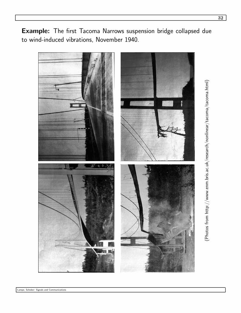
32

Example: The first Tacoma Narrows suspension bridge collapsed due

to wind-induced vibrations, November 1940.

(Phot

osfrom

htt

p:/

/ww

w.e

nm

.bris.ac

.uk/

rese

arch

/non

linea

r/ta

com

a/ta

com

a.htm

l)


1 signals and systems - kauno technologijos …girrol/skaidres/literatura/angliska/pateiktys/... ·...

Documents