1

Self-triggered Feedback Control Systems with

Finite-GainL2 Stability

Xiaofeng Wang and M.D. Lemmon

Abstract

This paper examines a class of real-time control systems in which each control task triggers its next

release based on the value of the last sampled state. Prior work [1] used simulations to demonstrate

that self-triggered control systems can be remarkably robust to task delay. This paper derives bounds

on a task’s sampling period and deadline to quantify how robust the control system’s performance will

be to variations in these parameters. In particular we establish inequality constraints on a control task’s

period and deadline whose satisfaction ensures that the closed loop system’s inducedL2 gain lies below

a specified performance threshold. The results apply to linear time-invariant systems driven by external

disturbances whose magnitude is bounded by a linear function of the system state’s norm. The plant

is regulated by a full-informationH∞ controller. These results can serve as the basis for the design

of soft real-time systems that guarantee closed-loop control system performance at levels traditionally

seen in hard real-time systems.

I. I NTRODUCTION

Computer-controlled systems are often implemented using periodic tasks satisfying hard real-

time constraints. Under a periodic task model, consecutive invocations (also called jobs) of a

task are released in a periodic manner. If the task model satisfies a hard real-time constraint, then

each job completes its execution by a specified deadline. Hard real-time periodic task models

allow the control system designer to treat the computer-controlled system as a discrete-time

system, for which there are a variety of mature controller synthesis methods.

Both authors are with the department of electrical engineering, University of Notre Dame, Notre Dame, IN 46556; e-mail:

xwang13,lemmon@nd.edu. The authors gratefully acknowledge the partial financial support of the National Science Foundation

(grants NSF-ECS-0400479 and NSF-CNS-0410771)

June 27, 2007 DRAFT

2

Periodic task models may be undesirable in many situations. Traditional approaches for

estimating task periods and deadlines are very conservative, so the control task may have greater

utilization than it actually needs. This results in significant over-provisioning of the real-time

system hardware. With such high utilization, it may be difficult to schedule other tasks on the

same processing system. Finally, it should be noted that real-time scheduling over networked

systems may be poorly served by the periodic task model. In many networked systems, tasks

are finished only after information has been successfully transported across the network. It is

often unreasonable to expect hard real-time guarantees on message delivery in communication

networks. This is particularly true for wireless sensor-actuator networks. In these applications,

there may be good reasons to consider alternatives to periodic task models.

This paper considers aself-triggered task model in which each task determines the release

of its next job. In reality, one might consider periodic task models as self-triggered tasks since

many implementations release tasks upon expiration of a one-shot timer that was started by

the previous invocation of the task. Under a periodic task model, the period of this one-shot

timer is always a constant value. This paper, however, considers a more adaptive form of self-

triggering in which the value loaded into the one-shot timer is actually a function of the system

state sampled by the current job. Under this “state-based” self-triggering, each task releases its

next job based on the system state. We can therefore consider “state-based” self-triggering as

a closed-loop form of releasing tasks for execution, whereas periodic task models release their

jobs in an open-loop fashion. For simplicity, this paper refers to a “state-based” self-triggered

task model as “self-triggered”.

Self-triggering provides a more flexible way of adjusting task periods. Since task periods

are based on the system’s current state, it is possible to reduce control task utilization during

periods of time when the system is sitting happily at its equilibrium point. The question here is

precisely how much freedom do we have in adjusting task periods in response to variations in

the system state. This paper answers that question by providing bounds on the task periods and

deadlines required to assure a specified level ofL2 stability. Our results pertain to linear time-

invariant system with state feedback. Since our controller seeks to ensureL2 stability, we use

a full-informationH∞ controller in our analysis. We also assume that the system has a process

noise whose magnitude is bounded by a linear function of the norm of the system state. Under

these assumptions we obtain a set of inequality constraints on the task period and deadlines as a

June 27, 2007 DRAFT

3

function of the system state. On the basis of simulation results, these bounds appear to be tight

and relatively easy to compute, so it may be possible to use them in actual real-time control

systems.

The remainder of this paper is organized as follows. Section II discusses the prior work related

to self-triggered feedback. Section III introduces the system model. Section IV derives sufficient

threshold condition that can serve as an event triggering state sampling. In section V, the self-

triggering scheme is presented and the system is shown to beL2 stable. Simulations are shown

in section VI. Finally, conclusions and future work are presented in section VII.

II. PRIOR WORK

To the best of our knowledge there is relatively little prior work examining state-based self-

triggered feedback control. A self-triggered task model was introduced by Velasco et al. [2]

in which a heuristic rule was used to adjust task periods. A self-triggered task model was also

introduced by Lemmon et al. [1] which chose task periods based on a Lyapunov-based technique.

But other than these two papers, we are aware of no other serious work looking at self-triggered

feedback schemes. There is, however, a great deal of related work dealing with so-called event-

triggered feedback, sample period selection, and real-time control system co-design. We’ll review

each of these areas in more detail below and then discuss their relationship to the self-triggered

task models.

Traditional methods for sample period selection [3] are usually based on Nyquist sampling.

Nyquist sampling ensures that the sampled signal can be perfectly reconstructed from its samples.

In practice, however, feedback within the control system means the system’s performance will

be somewhat insensitive to errors in the feedback signal, so that perfect reconstruction is much

more than we require in a feedback control system. An alternative approach to the sample

period selection problem makes use of Lyapunov techniques. This was done in Zheng et al.

[4] for a class of nonlinear sampled-data system. Nesic et al. [5] used input-to-state stability

(ISS) techniques to bound the inter-sample behavior of nonlinear systems. The sample periods

obtained by these methods also tend to be very conservative due to the bounding techniques

used.

The prior work on sample-period selection using Lyapunov methods can determine sampling

periods ensuring asymptotic stability in nonlinear systems. For the linear systems we consider,

June 27, 2007 DRAFT

4

these methods can yield very tight estimates on the sampling period. This was actually demon-

strated by Tabuada et al. [6] and the basic technique employed by Tabuada to estimate sample

periods is used in this paper as well.

Another related research direction viewed sample period selection as a “co-design” problem

that involves both the control system and the real-time system. In this case, sample periods are

selected to minimize some penalty on control system performance subject to a schedulability

condition. Early statements of this problem may be found in Seto et al. [7] with more recent

studies in [8] and [9]. The penalty function is often a performance index for an infinite horizon

optimal control problem. It has, however, been demonstrated [10] that such indices are rarely

monotone functions of the sampling period. As a result, it only appears to be feasible to do

off-line determination of these “optimal” sampling periods.

The prior work on co-design really focuses on optimizing performance subject to scheduling

constraints. The scheduling constraints are Liu-Layland [11] schedulability conditions for earliest

deadline first (EDF) scheduling. It is not always clear, however, that these are the best set of

constraints to be using. This paper actually derives a set of constraints on both the periods

and deadlines that we can then use as a quality-of-service (QoS) constraint that the real-time

scheduler needs to meet. We do not address the schedulability of these QoS constraints in this

paper, though that is an important research issue that we are still studying.

In recent years, a number of researchers have proposed aperiodic and sporadic task models in

which tasks are event-triggered [12]. By event-triggering, we usually mean that the system state is

sampled when some function of the system state exceeds a threshold. The idea of event-triggered

feedback has appeared under a variety of names, such as interrupt-based feedback [13], Lebesgue

sampling [14], asynchronous sampling [15], or state-triggered feedback [6]. Event triggering

usually requires some form of hardware event detector to generate a hardware interrupt to release

the control task. This can be done using either custom analog integrated circuits (ASIC’s) or

floating point gate array (FPGA) processors.

The prior work on event-triggered feedback is probably most closely related to this paper’s

work. In particular, the bounds we derive in this paper are based on variations of the event-

triggering conditions used by Tabuada et al. [6]. The conditions given in our paper appear to be

less conservative than the bounds obtained in [6].

June 27, 2007 DRAFT

5

III. SYSTEM MODEL

Consider a linear time-invariant system whose statex : < → <n satisfies the initial value

problem,

x(t) = Ax(t) + Bu(t) + w(t)

x(0) = x0

whereu : < → <m is a control input andw : < → <n is an exogenous disturbance function

in L2 such that there exists a positive real constantW > 0 so that‖w(t)‖2 ≤ W‖x(t)‖2 for

all t ≥ 0. In the above equation,A ∈ <n×n and B ∈ <n×m are real matrices of appropriate

dimensions.

Since we’re interested in controllers that are finite-gainL2 stable, we assume there exists a

full-informationH∞ controller that asymptotically stabilizes the unforced system. In particular,

we assume there exists a symmetric positive definite matrixP such that

x(t) = (A−BBT P )x(t) (1)

has an asymptotically stable equilibrium. The matrixP satisfies theH∞ algebraic Riccati

equation (ARE),

0 = PA + AT P −Q + R (2)

where

Q = PBBT P (3)

R = I +1

γ2PP (4)

for some real constantγ > 0. For notational convenience the system matrix of the closed loop

system (equation 1) will be denoted asAcl = A − BBT P . The state feedback gain matrix is

K = −BT P .

If we consider the standardL2 storage functionV : <n → < given byV (x) = xT Px for all

x ∈ <n then the preceding assumptions aboutP allow us to show that the storage function’s

directional derivative satisfies the dissipative inequality,

V (x(t)) < −‖x(t)‖22 + γ2‖w(t)‖2

2 (5)

June 27, 2007 DRAFT

6

for all t. Recall that a linear system,T , is said to be finite gainL2 stable ifT is a linear operator

from L2 back intoL2. The induced gain ofT is

‖T‖ = sup‖w‖L2

=1‖Tw‖L2 .

Satisfaction of the dissipative inequality (eq. 5) is sufficient to show that the systemT charac-

terized by the state equation

x(t) = (A−BBT P )x(t) + w(t) (6)

is finite gainL2 stable with an induced gain less thanγ.

This paper considers a sampled-data implementation of the closed loop system in equation 6.

This means that the plant’s control,u, is computed by a computer task. This task is characterized

by two monotone increasing sequences of time instants; the release time sequence{rk}∞k=0 and the

finishing time sequence{fk}∞k=0. We say these two sequences are admissible ifrk ≤ fk < rk+1

for all k = 0, . . . ,∞. The timerk denotes the time when thekth invocation of a control task

(also called a job) is released for execution on the computer’s central processing unit (CPU). At

this time, we assume that the system state is sampled so thatrk also represents thekth sampling

time instant. The timefk denotes the time when thenkth job has finished executing. Each job

of the control task computes the controlu based on the last sampled state. Upon finishing, the

control job outputs this control to the plant. The control signal used by the plant is held constant

by a zero-order hold (ZOH) until the next finishing timefk+1. This means that the sampled-data

system under study in this project satisfies the following set of state equations,

x(t) = Ax(t) + Bu(t) + w(t) (7)

u(t) = −BT Px(rk)

for t ∈ [fk, fk+1) and all k = 0, . . . ,∞. The state trajectoriesx satisfying equation 7 are

continuous so that the initial state at timefk is simply x(fk) = limt↑fkx(t).

We let Tk = rk+1 − rk denote thekth inter-release time (k = 0, . . . ,∞). Tk can therefore be

interpreted as a time-varying “sampling” period by control engineers and a time-varying “task”

period by real-time system engineers. We letDk = fk − rk denote the time interval between

the kth job’s release and finishing time. Control engineers would viewDk as the “delay” of the

kth job whereas real-time system engineers would viewDk as the “jitter” of thekth job. If the

June 27, 2007 DRAFT

7

control task satisfies a hard real-time constraint, then the delayDk is required to lie below a

specified “deadline”.

If we decrease the sampling period,Tk, and delay,Dk, in a uniform manner so that the resulting

release and finishing time sequences remain admissible, then the state trajectories generated by

the sampled-data system in equation 7 will converge to state trajectories satisfying the original

closed-loop system equation 6. By construction of the control, we know that this original system

is L2 stable with gain less thanγ. This paper’s main results establish nontrivial bounds on

the sequence of sampling periods{Tk}∞k=0 and delays{Dk}∞k=0 such that the resulting release

and finishing time sequences are admissible and the sampled-data system preserves the original

system’sL2 stability.

IV. L2 STABILITY

Consider the sampled-data system in equation 7 with a set of admissible release and finishing

time sequences. For allk, define thekth job’s error functionek : [rk, fk+1) → <n by ek(t) =

x(t)−x(rk). This error represents the difference between the current system state and the system

state at the last release time,rk. This section presents two inequality constraints onek(t) (see

theorem 4.1 and corollary 4.2 below) whose satisfaction is sufficient to ensure that the sampled-

data system’sL2 gain is less thanγ/β for some parameterβ ∈ (0, 1].

Notational conventions: The sufficient conditions derived in this section apply uniformly

to all jobs, k. We may therefore, for notational convenience, drop the job indexk with the

understanding that we’re only considering thekth job’s error signal. In particular, the times

rk−1, rk, rk+1, fk, andfk+1 will be denoted asr−, r, r+, f , andf+, respectively. The system

state at timet ∈ [rk, fk+1) will be denoted asxt and thekth job’s error signal,ek(t), at time t

will be denoted aset = xt − xr for t ∈ [r, f+).

The following theorem states that if a function of the state errorek(t) and statex(t) satisfies

a certain inequality constraint, then the closed loop system in equation 7 is finite gainL2 stable.

Theorem 4.1:Consider the sampled-data system in equation 7 with admissible release and

finishing time sequences. Letβ be any real constant in the open interval(0, 1) with the matrix

Q as given in equation 3. If

eTk (t)Qek(t) < (1− β2)‖x(t)‖2

2 + xTr Qxr (8)

June 27, 2007 DRAFT

8

for all t ∈ [fk, fk+1) and anyk = 0, . . . ,∞, then the sampled-data system is finite gainL2 stable

with a gain less thanγ/β.

Proof: Consider the storage functionV : <n → < given by V (x) = xT Px for x ∈ <n

whereP is a symmetric positive definite matrix satisfying the algebraic Riccati equation (eq.

2). The directional derivative ofV for t ∈ [fk, fk+1) is

V =∂V

∂x

(Axt −BBT Pxr + w

)

= −xTt

(I −Q +

1

γ2PP

)xt − 2x(t)T Qxr + 2xT

t Pw

= −xTt (I −Q)xt −

∥∥∥∥∥γwt − 1

γPxt

∥∥∥∥∥2

2

+ γ2‖wt‖22 − 2xT

t Qxr

≤ −xTt (I −Q)xt + γ2‖wt‖2

2 − 2xTt Qxr (9)

Insertxt = et + xr into the above equation to obtain

V ≤ −‖xt‖22 + [et + xr]

T Q [et + xr]− 2 [et + xr]T Qr + γ2‖wt‖2

2

= −‖xt‖22 + eT

t Qet − xTr Qxr + γ2‖wt‖2

2 (10)

By the assumption in equation 8, we know that equation 10 can be rewritten as

V ≤ −β2‖xt‖22 + γ2‖wt‖2

2 (11)

This is the dissipative inequality that holds for allt and is sufficient to ensure the sampled-data

system isL2 stable with a gain less thanγ/β.

In our following work, we’ll find it convenient to use a slightly weaker sufficient condition

for L2 stability which is only a function of the state errorek(t). The following corollary states

this result.

Corollary 4.2: Consider the sampled-data system in equation 7 with admissible sequences of

release and finishing times. LetQ be a real matrix that satisfies equation 3 andβ be a real

constant in the interval(0, 1] such that the matrix

M = (1− β2)I + Q. (12)

has full rank. If the state error trajectory satisfies

ek(t)T Mek(t) ≤ xT

r Mxr (13)

June 27, 2007 DRAFT

9

for t ∈ [fk, fk+1) for all k = 0, . . . ,∞, then the sampled data system isL2 stable with a gain

less thanγ/β.

Proof: Equation 13 can be rewritten as

ek(t)T Mek(t) = (1− β2)‖ek(t)‖2

2 + ek(t)T Qek(t)

≤ (1− β2)‖xr‖22 + xT

r Qxr

This can be rewritten to obtain

ek(t)T Qek(t) ≤ (1− β2)(‖xr‖2

2 − ‖ek(t)‖22) + xT

r Qxr

≤ (1− β2)‖x(t)‖22 + xT

r Qxr

where we used the fact that

‖xr‖22 − ‖et‖2

2 ≤ ‖xr + et‖22 = ‖x(t)‖2

2.

This inequality is the sufficient condition in theorem 4.1 so we can conclude that the sampled-

data system isL2 stable with a gain less thanγ/β.

Remark 4.3:The inequalities in equations 8 or 13 can both be used as the basis for an event-

triggered feedback control system (section II). Note that both inequalities are trivially satisfied at

t = rk. If we let the delay,Dk, be zero for each job, then by triggering the release times{rk}∞k=0

anytime before the inequalities in equations 8 or 13 are violated, we will ensure the sampled-data

system’s inducedL2 gain remains belowγ/β. The resulting event-triggered feedback system

is very similar to the state-triggering scheme proposed by Tabuada et al. [6] for asymptotic

stability. The main difference between that result and this one is that our proposed event-

triggering condition provides a stronger assurance on the sampled-data system’s performance

as measured by its inducedL2 gain. Another important difference is that the threshold condition

in equation 13 is stated in terms of the last sampled state,xr. The corresponding threshold

condition in [6] is given in terms of the current statext. This difference makes it easier to

convert our event-triggering condition into a self-triggered feedback scheme.

V. A DMISSIBLE RELEASE AND FINISHING TIMES

This section establishes sufficient conditions for the existence of admissible sequences of

release and finishing times that ensure the sampled data system in equation 7 isL2 stable with

June 27, 2007 DRAFT

10

a specified gain. These conditions take the form of admissible bounds on the task sampling

periods,Tk, and task delays,Dk.

For notational convenience letzk : [rk, fk+1) → <n be given as

zk(t) =√

(1− β2)I + Q =√

Mek(t) (14)

where√

M is a matrix square root andM is defined in equation 12. We refer tozk as thekth

job’s “trigger signal”. Note thatM is dependent on the paramterβ.

We define the functionρ : <n → < given by

ρ(x) =√

xT Mx (15)

wherex ∈ <n. So if we can guarantee for anyδ ∈ (0, 1] that

‖zk(t)‖2 ≤ δρ(xr) (16)

for all t ∈ [fk, fk+1) for any k = 0, . . . ,∞, then the hypotheses in corollary 4.2 are satisfied

and we can conclude that the sampled-data system is finite-gainL2 stable with a gain less than

γ/β.

The first major result examines what happens if we use equation 16 as the basis for an

event-triggered feedback control system. In particular, let’s assume that thekth job’s release,rk,

is precisely that time when‖zk(t)‖2 = δρ(xr) under the assumption that thekth job’s delay,

Dk, is zero. The following theorem states a lower bound on the sampling period for which a

sampled-data system with zero delay (i.e.Dk = 0) has an inducedL2 gain less thanγ/β.

Theorem 5.1:Consider the sampled-data system in equation 7 and assume there exists a non-

negative real constantW such that‖wt‖2 ≤ W‖xt‖2 for all t ∈ <. Assume that for some

δ ∈ (0, 1] that the sequence of release times{rk}∞k=0 satisfy

‖z(rk+1)‖2 = δρ(xr) (17)

wherefk = rk for all k = 0, . . . ,∞.

The sequence of release and finishing times is admissible and the sampled-data system is

L2-stable with a gain less thanγ/β. Furthermore, the task sampling periods satisfy

Tk ≥ 1

αln

(1 + δα

ρ(xr)

µ0(xr)

)(18)

June 27, 2007 DRAFT

11

whereα is a real constant

α =∥∥∥∥√

MA√

M−1

∥∥∥∥ + W∥∥∥√

M∥∥∥

∥∥∥∥√

M−1

∥∥∥∥ (19)

andµ0 : <n → < is a real-valued function given by

µ0(xr) =∥∥∥√

MAclxr

∥∥∥2+ W

∥∥∥√

M∥∥∥ ‖xr‖2 . (20)

Proof: The time derivative of‖zk(t)‖2 for t ∈ [r, f+) satisfies

d

dt‖zk(t)‖2 ≤

∥∥∥√

Mek(t)∥∥∥2

=∥∥∥√

Mxt

∥∥∥2

=∥∥∥√

M(Axt −BBT Pxr + wt

)∥∥∥2

≤∥∥∥√

MAek(t)∥∥∥2+

∥∥∥√

MAclxr

∥∥∥2+

∥∥∥√

M∥∥∥ ‖wt‖2 (21)

Since‖wt‖2 ≤ W‖xt‖2, xt = ek(t) + xr, and zk(t) =√

Mek(t), we can bound the preceding

equation (21) as

d

dt‖zk(t)‖2 ≤

∥∥∥∥√

MA√

M−1

∥∥∥∥ ‖zk(t)‖2 +∥∥∥√

MAclxr

∥∥∥2

+W(‖√

M‖‖√

M−1

zk(t)‖2 + ‖√

M‖‖xr‖2

)

=(∥∥∥∥√

MA√

M−1

∥∥∥∥ + W‖√

M‖‖√

M−1‖

)‖zk(t)‖2

+∥∥∥√

MAclxr

∥∥∥2+ W

∥∥∥√

M∥∥∥ ‖xr‖2

= α‖zk(t)‖2 + µ0(xr). (22)

whereα andµ0 : <n → < are defined in equations 19 and 20, respectively.

The initial condition is‖zk(r)‖2 = 0. Using this in the differential inequality (eq. 22) yields,

‖zk(t)‖2 ≤ µ0(xr)

α

(eα(t−r) − 1

)(23)

for all t ∈ [r, f+).

By assumptionr+ = f+ (i.e. no task delay) andδρ(xr) = ‖zk(r+)‖2, so we can conclude

that

δρ(xr) = ‖zk(r+)‖2 ≤ µ0(xr)

α

(eαTk − 1

)(24)

whereTk = r+ − r is the task sampling period for jobk. Solving equation 24 forTk yields

equation 18. The righthand side of the inequality 18 is clearly strictly greater than zero, which

implies thatrk+1 − rk > 0. Thereforerk = fk ≤ rk+1 which implies that the sequence of

June 27, 2007 DRAFT

12

finishing and release times is admissible. Finally we know that‖zk(t)‖2 ≤ δρ(xr) for all t ∈[rk, fk+1) = [fk, fk+1) and allk = 0, . . . ,∞, which by corollary 4.2 implies that the system is

L2 stable with a gain less thanγ/β.

Remark 5.2:Note that the righthand side of equation 18 will always be strictly greater than

zero. We can therefore conclude that if we trigger release times whenδρ(xr) = ‖zk(r+)‖, then

the sampling periodTk can never be zero.

Remark 5.3:The admissibility of sequences{rk}∞k=0 and{fk}∞k=0 can be restated in terms of

the sequences{Dk}∞k=0 and{Tk}∞k=0. By definition, the release and finishing time sequences are

admissible if and only ifrk ≤ fk ≤ rk+1 for all k. Clearly this holds if and only if0 ≤ Dk ≤ Tk

for all k.

The previous theorem presumes there is no task delay (i.e.Dk = 0). Under this assumption,

theorem 5.1 states that triggering release times when equation 17 holds assures the closed-loop

system’s inducedL2 gain. This theorem, however, also provides a lower bound on the task

sampling period, which suggests that we can also use theorem 5.1 as the basis for state-based

self-triggered feedback. In this scenario, if thekth job would set the next job’s release time as

rk+1 = rk +1

αln

(1 + δα

ρ(xr)

µ0(xr)

)(25)

then we are again assured of the system’s inducedL2 gain is less thanγ/β.

The problem faced in using equation 25 for self-triggering is the assumption of no task delay. In

many application, task delay may not be small enough to neglect. If we consider non-zero delay,

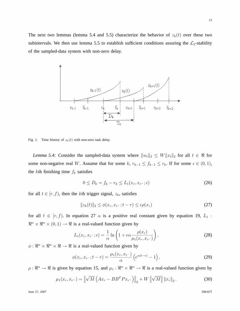
then the triggering signals appear as shown in figure 1. This figure shows the time history for

the triggering signals,zk−1, zk, andzk+1. With non-zero delay, we can partition the time interval

[rk, fk+1) into two subintervals[rk, fk) and [fk, fk+1). The differential equations associated with

subintervals[rk, fk) and [fk, fk+1) are

x(t) = Ax(t)−BBT Pxr− + w(t)

and

x(t) = Ax(t)−BBT Pxr + w(t),

respectively. In a manner similar to the proof of theorem 5.1, we can use differential inequalities

to boundzk(t) for all t ∈ [rk, fk+1) and thereby determine sufficient conditions assuring the

admissibility of the release/finishing times while preserving the closed-loop system’sL2-stability.

June 27, 2007 DRAFT

13

The next two lemmas (lemma 5.4 and 5.5) characterize the behavior ofzk(t) over these two

subintervals. We then use lemma 5.5 to establish sufficient conditions assuring theL2-stability

of the sampled-data system with non-zero delay.

Fig. 1. Time history ofzk(t) with non-zero task delay.

Lemma 5.4:Consider the sampled-data system where‖wt‖2 ≤ W‖xt‖2 for all t ∈ < for

some non-negative realW . Assume that for somek, rk−1 ≤ fk−1 ≤ rk. If for someε ∈ (0, 1),

the kth finishing timefk satisfies

0 ≤ Dk = fk − rk ≤ L1(xr, xr− ; ε) (26)

for all t ∈ [r, f), then thekth trigger signal,zk, satisfies

‖zk(t)‖2 ≤ φ(xr, xr− ; t− r) ≤ ερ(xr) (27)

for all t ∈ [r, f). In equation 27α is a positive real constant given by equation 19,L1 :

<n ×<n × (0, 1) → < is a real-valued function given by

L1(xr, xr− ; ε) =1

αln

(1 + εα

ρ(xr)

µ1(xr, xr−)

), (28)

φ : <n ×<n ×< → < is a real-valued function given by

φ(xr, xr− ; t− r) =µ1(xr, xr−)

α

(eα(t−r) − 1

), (29)

ρ : <n → < is given by equation 15, andµ1 : <n ×<n → < is a real-valued function given by

µ1(xr, xr−) =∥∥∥√

M(Axr −BBT Pxr−

)∥∥∥2+ W

∥∥∥√

M∥∥∥ ‖xr‖2 . (30)

June 27, 2007 DRAFT

14

Proof: For t ∈ [r, f), the derivative of‖zk(t)‖2 satisfies the differential inequality,

d

dt‖zk(t)‖2 ≤ ‖zk(t)‖2 =

∥∥∥√

Mek(t)∥∥∥2

=∥∥∥√

Mx(t)∥∥∥2

=∥∥∥√

M(Axt −BBT Pxr− + wt

)∥∥∥2

=∥∥∥√

M(Aek(t) + Axr −BBT Pxr− + wt

)∥∥∥2

≤(∥∥∥∥√

MA√

M−1

∥∥∥∥ + W∥∥∥√

M∥∥∥

∥∥∥∥√

M−1

∥∥∥∥)‖zk(t)‖2

+∥∥∥√

M(Axr −BBT Pxr−

)∥∥∥2+ W

∥∥∥√

M∥∥∥ ‖xr‖2

= α‖zk(t)‖2 + µ1(xr, xr−). (31)

The differential inequality in equation 31 along with the initial conditionzk(r) = 0, allows us

to conclude that

‖zk(t)‖2 ≤ φ(xr, xr− ; t− r) (32)

for all t ∈ [r, f).

The assumption in equation 26 can be rewritten as

φ(xr, xr− ; Dk) ≤ ερ(xr) (33)

φ(xr, xr− ; t− r) is a monotone increasing function oft− r. Combining this fact with equations

32 and 33 yields

‖zk(t)‖2 ≤ φ(xr, xr− ; t− r) ≤ φ(xr, xr− ; Dk) ≤ ερ(xr)

which leads to equation 27 holding for allt ∈ [r, f).

Lemma 5.5:Consider the sampled-data system in equation 7 where‖wt‖2 ≤ W‖xt‖2 for some

non-negative realW . For a given integerk and someε ∈ (0, 1), assume thatrk−1 ≤ fk−1 ≤ r.

For anyη ∈ (ε, 1], let

dη = fk + L2(xr, xr− ; Dk, η), (34)

whereL2 : <n ×<n ×<× (0, 1] → < is given by

L2(xr, xr− ; Dk, η) =1

αln

(1 + α

ηρ(xr)− φ(xr, xr− ; Dk)

µ0(xr) + αφ(xr, xr− ; Dk)

). (35)

June 27, 2007 DRAFT

15

if

0 ≤ Dk ≤ L1(xr, xr− ; ε) (36)

then

dη > fk, and (37)

‖zk(t)‖2 ≤ ηρ(xr) for all t ∈ [fk, dη] (38)

Proof: The hypotheses of this lemma also satisfy the hypotheses of lemma 5.4 so we know

that

‖zk(f)‖2 ≤ φ(xr, xr− ; Dk) ≤ ερ(xr) ≤ ηρ(xr). (39)

By equation 35 and 39, we have

L2(xr, xr− ; Dk, η) > 0

which implies

dη > fk

Assume the system statext satisfies the differential equation

xt = Axt −BBT Pxr + wt

for t ∈ [fk, dη]. Using an argument similar to that in lemma 5.4, we can show that‖zk(t)‖2

satisfies the differential inequality

d

dt‖zk(t)‖2 ≤ α‖zk(t)‖2 + µ0(xr). (40)

Equation 39 can be viewed as an initial condition on the differential inequality in equation

40. Solving the differential inequality, we know for allt ∈ [fk, dη],

‖zk(t)‖2 ≤ eα(t−f)φ(xr, xr− ; Dk) +µ0(xr)

α

(eα(t−f) − 1

). (41)

Because the right side of equation 41 is an increasing function oft, we get

‖zk(t)‖2 ≤ eα(dη−f)φ(xr, xr− ; Dk) +µ0(xr)

α

(eα(dη−f) − 1

)= ηρ(xr). (42)

for all t ∈ [fk, dη].

June 27, 2007 DRAFT

16

According to lemma 5.5, for a constantδ ∈ (ε, 1), if r+ = f + L2(xr, xr− ; Dk, δ) andf+ ≤f + L2(xr, xr− ; Dk, 1), we will always have‖zk(r

+)‖2 ≤ δρ(xr) and ‖zk(f+)‖2 ≤ ρ(xr). We

will use this fact below to characterize a self-triggering scheme that preserves the sampled-data

system inducedL2 gain. Theorem 5.7 formally states this self-triggering scheme. The proof of

theorem 5.7 requires the following lemma showing that the longest allowable task delay given

in lemma 5.4 is bounded below by a positive function ofxr−.

Lemma 5.6:Consider the sampled-data system where‖wt‖2 ≤ W‖xt‖2 for all t ∈ < where

W is a non-negative real constant. Assume that for a constantδ ∈ (ε, 1), the release timer−

andr satisfy

‖zk−1(r)‖2 ≤ δρ(xr−) (43)

for any givenk. Then there exists a functionξ : <n× (0, 1)× (0, 1) → <+ such that the function

L1 : <n ×<n × (0, 1) → < given by equation 28 satisfies the bound

L1(xr, xr− ; ε) ≥ ξ(xr− ; ε, δ) > 0. (44)

Proof: First note thatxr = ek−1(r) + xr− implies that

‖xr−‖2 − ‖ek−1(r)‖2 ≤ ‖xr‖2 ≤ ‖xr−‖2 + ‖ek−1(r)‖2

We now use this inequality to boundρ(xr) andµ1(xr, xr−) as a function ofxr−.

A lower bound onρ(xr) is obtained by noting that

ρ(xr) =∥∥∥√

Mxr

∥∥∥2

=∥∥∥√

M(ek−1(r) + xr−)∥∥∥2

≥ ‖√

Mxr−‖2 − ‖zk−1(r)‖2

≥ ρ(xr−)− δρ(xr−) (45)

= (1− δ)ρ(xr−) ≡ ξ1(xr− ; δ) (46)

An upper bound onµ1(xr, xr−) can be obtained by noting that

µ1(xr, xr−) =∥∥∥√

M(Axr −BBT Pxr−

)∥∥∥2+ W‖

√M‖‖xr‖2

=∥∥∥√

M (Aclxr− + Aek−1(r))∥∥∥2+ W‖

√M‖‖xr− + ek−1(r)‖2

≤∥∥∥√

MAclxr−∥∥∥ + W‖

√M‖‖xr−‖2

+∥∥∥∥√

MA√

M−1

zk−1(r)∥∥∥∥2+ W‖

√M‖‖

√M

−1zk−1(r)‖2

June 27, 2007 DRAFT

17

≤∥∥∥√

MAclxr−∥∥∥ + W‖

√M‖‖xr−‖2

+(∥∥∥∥√

MA√

M−1

∥∥∥∥ + W‖√

M‖‖√

M−1‖

)δρ(xr−)

= µ0(xr−) + αδρ(xr−) ≡ ξ2(xr− ; δ) (47)

Putting both inequalities together we see that

L1(xr, xr− ; ε) =1

αln

(1 + εα

ρ(xr)

µ1(xr, xr−)

)

≥ 1

αln

(1 + εα

ξ1(xr− ; δ)

ξ2(xr− ; δ)

)

=1

αln

(1 + εα

(1− δ)ρ(xr−)

αδρ(xr−) + µ0(xr−)

)≡ ξ(xr− ; ε, δ) > 0 (48)

which completes the proof.

With the preceding technical lemma we can now state a self-triggered feedback scheme which

can guarantee the sampled-data system’s inducedL2 gain. The basis for this self-triggering

scheme will be found in the following theorem.

Theorem 5.7:Consider the sampled-data system in equation 7 where‖wt‖2 ≤ W‖xt‖2 for

all t ∈ <+ whereW is some non-negative real constant. For givenε ∈ (0, 1) andδ ∈ (ε, 1), we

assume that

• The initial release and finishing times satisfy

r−1 = r0 = f0 = 0

• For any non-negative integerk, the release times are generated by the following recursion,

rk+1 = fk + L2(x(rk), x(rk−1); Dk, δ) (49)

and the finishing times satisfy

rk+1 ≤ fk+1 ≤ rk+1 + ξ(x(rk); ε, δ). (50)

whereL2 is given in equation 35 andξ is given in equation 48. Then the sequence of release

times,{rk}∞k=0, and finishing time,{fk}∞k=0, will be admissible and the sampled-data system is

finite gainL2 stable with an induced gain less thanγ/β.

Proof: From the definition ofξ in equation 48, we can easily see thatξ(xr; ε, δ) > 0

for any non-negative integerk. We can therefore use equation 50 to conclude that the interval

[rk+1, rk+1 + ξ(xr; ε, δ)] is nonempty for allk.

June 27, 2007 DRAFT

18

Next, we insert equation 49 into equation 50 to show that

fk+1 ≤ rk+1 + ξ(x(rk); ε, δ)

≤ fk + L2(x(rk), x(rk−1); Dk, δ) + ξ(x(rk)); ε, δ)

= fk + L2(x(rk), x(rk−1); Dk, 1) (51)

for all non-negative integersk.

With the preceding two preliminary results, we now consider the following statement about

the kth job. This statement is that

1) rk ≤ fk ≤ rk+1,

2) ‖zk(t)‖2 ≤ δρ(x(rk)) for all t ∈ [fk, rk+1],

3) and‖zk(t)‖2 ≤ ρ(x(rk)) for all t ∈ [fk, fk+1].

We now use mathematical induction to show that under the theorem’s hypotheses, this statement

holds for all non-negative integersk.

First consider the base case whenk = 0. According to the definition ofL2 (equation 35) we

know that

L2(x0, x0; D0, δ) = L2(x0, x0; Dk, δ) > 0

We can therefore combine equations 50 and 49 to obtain

r0 = f0 ≤ f0 + L2(x0, x0; D0, δ) = r1 (52)

which establishes the first part of the inductive statement whenk = 0.

Next note that

D0 = 0 ≤ L1(x(r0), x(r−1); ε). (53)

If we use the fact thatδ ∈ (ε, 1) ⊂ (0, 1] in equations 49 and 53, we can see that the hypotheses

of lemma 5.5 are satisfied. This means that‖z0(t)‖2 ≤ δρ(x(r0)) for all t ∈ [f0, r1] which

completes the second part of the inductive statement fork = 0.

Now define the time

d01 = f0 + L2(x(r0), x(r−1); D0, 1)

Equation 53 again implies that the hypotheses of lemma 5.5 are satisfied, so that

‖z0(t)‖2 ≤ ρ(x(r0)) for all t ∈ [f0, d01]. (54)

June 27, 2007 DRAFT

19

From equation 51, we know thatf1 ≤ d01. We can also combine equations 50 and 52 to conclude

thatf0 ≤ f1. We therefore know that[f0, f1] ⊆ [f1, d01] which combined with equation 54 implies

that

‖z0(t)‖2 ≤ ρ(x(r0)) for all t ∈ [f1, d01]

This therefore establishes the last part of the inductive statement fork = 0.

We now turn to the general case for anyk. For a givenk let’s assume that the statement

holds. This means that

rk ≤ fk ≤ rk+1 (55)

‖zk(t)‖2 ≤ δρ(x(rk)) for all t ∈ [fk, rk+1] (56)

‖zk(t)‖2 ≤ ρ(x(rk)) for all t ∈ [fk, fk+1] (57)

Now consider thek + 1st job. Because equation 56 is true, the hypothesis of lemma 5.6 is

satisfied which means there exists a functionξ (given by equation 48) such that

0 < ξ(x(rk)); ε, δ) ≤ L1(x(rk+1), x(rk); ε).

We can use this in equation 50 to obtain

0 ≤ Dk+1 = fk+1 − rk+1 ≤ ξ(x(rk); ε, δ) ≤ L1(x(rk+1), x(rk); ε). (58)

From equation 58 and the fact thatδ ∈ (0, 1) we know that the hypotheses of lemma 5.5 hold

and we can conclude that

fk+1 ≤ rk+2 (59)

‖zk+1‖2 ≤ δρ(x(rk+1)) for all t ∈ [fk+1, rk+2]. (60)

Combining equation 50 with the above equation 59 yieldsrk+1 ≤ fk+1 ≤ rk+2 which establishes

the first part of the statement for the casek +1. Equation 60 is the second part of the statement.

Finally let

dk+11 = fk+1 + L2(x(rk+1), x(rk); Dk+1, 1)

Following our prior argument for the case whenk = 0, we know that the validity of equation

58 satisfies the hypotheses of lemma 5.5. We can therefore conclude that

‖zk+1(t)‖2 ≤ ρ(x(rk+1)) for all t ∈ [fk+1, dk+11 ] (61)

June 27, 2007 DRAFT

20

According to equation 51,fk+2 ≤ dk+11 . We can therefore combine equations 50 and 59 to

show thatfk+1 ≤ fk+2 and therefore conclude that[fk+1, fk+2] ⊆ [fk+1, dk+11 ]. Combining this

observation with equation 61 yields‖zk+1(t)‖2 ≤ ρ(x(rk+1)) for all t ∈ [fk+1, fk+2] which

completes the third part of the inductive statement for casek + 1.

We may therefore use mathematical induction to conclude that the inductive statement holds

for all non-negative integersk. The first part of the statement, of course, simply means that the

sequences{rk}∞k=0 and{fk}∞k=0 are admissible. The third part of the inductive statement implies

that the hypotheses of corollary 4.2 are satisfies, thereby ensuring that the system’s inducedL2

gain is less thanγ/β.

Remark 5.8:ξ(xr; ε, δ) serves as the deadline for the delayDk in theorem 5.7.

Remark 5.9:By the way we constructedδ, we see that it controls when the next job’s finishing

time. We might therefore expect to see a largerδ result in larger sampling periods. This is indeed

confirmed by the analysis. Since

Tk ≥ rk+1 − fk = L2(xr, xr− ; Dk, δ)

and sinceL2 is an increasing function ofδ we can see that largerδ result in larger sampling

periods.

Remark 5.10:By our construction of the parameterε, we see that it controls the current job’s

finishing time. Since this

Dk = fk − rk ≤ ξ(xr; ε, δ)

and sinceξ is an increasing function ofε, we can expect to see the allowable delay increase as

we increaseε. Note also thatξ is a decreasing function ofδ so that adopting a longer sampling

period by increasingδ will have the effect of reducing the maximum allowable task delay.

The following corollary to the above theorem shows that the task periods and deadlines

generated by our self-triggered scheme are all bounded away from zero. This is important in

establishing that our scheme does not generate infinite sampling frequencies.

Corollary 5.11: Assume the assumptions in theorem 5.7 hold. Then there exist two positive

constantsζ1, ζ2 > 0 such that

Tk ≥ ζ1

June 27, 2007 DRAFT

21

and

ξ(xr; ε, δ) ≥ ζ2

Proof: From theorem 5.7, we know

fk − rk ≤ ξ(xr; ε, δ) ≤ L1(xr, xr− ; ε)

Therefore, by lemma 5.4,

‖zk(f)‖2 ≤ φ(xr, xr− ; Dk) ≤ ερ(xr)

Let us first take a look atTk. From equation 49, we have

Tk ≥ rk+1 − fk

= L2(xr, xr− ; Dk, δ)

=1

αln

(1 + α

δρ(xr)− φ(xr, xr− ; Dk)

µ0(xr) + αφ(xr, xr− ; Dk)

)

≥ 1

αln

(1 + α

δρ(xr)− ερ(xr)

µ0(xr) + αερ(xr)

)

≥ 1

αln

(1 + α

(δ − ε)λ(√

M)‖xr‖2

‖√MAcl‖‖xr‖2 + W‖√M‖‖xr‖2 + αελ(√

M)‖xr‖2

)

=1

αln

(1 + α

(δ − ε)λ(√

M)

‖√MAcl‖+ W‖√M‖+ αελ(√

M)

)

= ζ1 > 0 (62)

It is easy to show that

ξ(xr; ε, δ) ≥ 1

αln

1 +

εα(1− δ)λ(√

M)∥∥∥√

MAcl

∥∥∥ + W‖√M‖+ δαλ(√

M)

= ζ2 > 0

VI. SIMULATION

The following simulation results were generated for event-triggered and self-triggered feedback

systems. The plant was an inverted pendulum on top of a moving cart. The plant’s linearized

state equations were

x(t) =

0 1 0 0

0 0 −mg/M 0

0 0 0 1

0 0 g/` 0

x(t) +

0

1/M

0

−1/(M`)

u(t) +

1

0

1

0

w(t)

June 27, 2007 DRAFT

22

whereM was the cart mass,m was the mass of the pendulum bob,` was the length of the

pendulum arm, andg was gravitational acceleration. For these simulations, we letM = 10, ` = 3,

andg = 10. The system state was the vectorx =[

y y θ θ

]T

wherey was the cart’s position

and θ was the pendulum bob’s angle with respect to the vertical. The control inputu(t) was

generated by either an event-triggered or self-triggered controller. The functionw was an external

disturbance to the system. The system’s initial state was the vectorx0 =[

0.98 0 0.2 0

]T

.

We designed a continuous-time state feedback control system (equation 1) in which the

performance level,γ, was set to200. Solving the Riccati equation in equation 2 yielded a

positive definite matrixP such that the state-feedback gains were

BT P =[−2 −12 −378 −210

].

The state trajectory of the resulting closed-loop system is denoted below asxc. Figure 2 plots

the system states as a function of time under the assumption thatw(t) = 0 for all t. Figure 2 is

therefore the impulse response of the inverted pendulum system.

0 5 10 15 20−0.5

0

0.5

1

1.5

2

2.5

3

3.5

t

ydy/dtθdθ/dt

Fig. 2. State Trajectories of Continuous-time Closed-loop System (eq. 1)

A. Event-triggered Feedback

This subsection presents simulation results for an event-triggered control of the inverted

pendulum. In this simulation, the next release (after releaser) was triggered when‖zk(t)‖2 =

δρ(xr) whereδ was set to0.7. Recall that the trigger signal,zk, is dependent on a parameterβ

(see equation 14). For all of the following simulations we letβ = 0.5. The task delays were set

June 27, 2007 DRAFT

23

equal to the deadline predicted in equation 48. In other wordsDk = ξ(x(rk−1; ε, δ) > 0 whereε

was chosen to be0.65. The external disturbance in this simulation was set to zero (i.e.w(t) = 0

for all t).

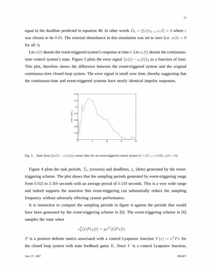
Let x(t) denote the event-triggered system’s response at timet. Letxc(t) denote the continuous-

time control system’s state. Figure 3 plots the error signal‖x(t)−xc(t)‖2 as a function of time.

This plot, therefore shows the difference between the event-triggered system and the original

continuous-time closed loop system. The error signal is small over time, thereby suggesting that

the continuous-time and event-triggered systems have nearly identical impulse responses.

0 5 10 15 200

0.02

0.04

0.06

0.08

0.1

0.12

0.14

t

|| x(

t) −

xc(t

) || 2

Fig. 3. State Error (‖x(t)− xc(t)‖2) versus time for an event-triggered control system (δ = 0.7, ε = 0.65, w(t) = 0)

Figure 4 plots the task periods,Tk, (crosses) and deadlines,ξ, (dots) generated by the event-

triggering scheme. The plot shows that the sampling periods generated by event-triggering range

from 0.023 to 2.368 seconds with an average period of0.349 seconds. This is a very wide range

and indeed supports the assertion that event-triggering can substantially reduce the sampling

frequency without adversely effecting system performance.

It is instructive to compare the sampling periods in figure 4 against the periods that would

have been generated by the event-triggering scheme in [6]. The event-triggering scheme in [6]

samples the state when

eTk (t)Pek(t) = pxT (t)Px(t).

P is a positive definite matrix associated with a control Lyapunov functionV (x) = xT Px for

the closed loop system with state feedback gainsK. SinceV is a control Lyapunov function,

June 27, 2007 DRAFT

24

0 5 10 15 2010

−3

10−2

10−1

100

101

t

Sampling PeriodPredicted Deadline

Fig. 4. Sampling periods and deadlines generated by event-triggered feedback (δ = 0.7, ε = 0.65, andw(t) = 0)

we can find a matrixH such that the directional derivative of the unforced closed loop system

satisfies the inequalityV ≤ −xT Hx. In the above equation,p is the real constant

p =λm(P )

2λM(P )

λm(H)

‖PBK‖whereλm(P ) andλM(P ) denote the minimum and maximum eigenvalues of matrixP , respec-

tively. For this particular simulation, we used theP associated with our controller to obtain

p = 4.17× 10−11. This event-triggering threshold generates sampling periods between10−6 and

10−4 seconds. This is much smaller than the sampling periods generated by event-triggering

using the threshold condition in corollary 4.2. The reason for this difference is that the condition

number of ourP matrix is extremely large due to the great difference in the time constants

associated with the dynamics of the cart and pendulum bob.

B. Self-triggered Feedback

The simulations in this subsection examined the self-triggering feedback scheme associated

with equations 49 and 50 in theorem 5.7. In this case the task release times were generated at

time fk using the equation

rk+1 = fk + L2(x(rk), x(rk−1), Dk, δ)

and the finishing times were required to satisfy

fk+1 = fk + ξ(x(rk); ε, δ)

June 27, 2007 DRAFT

25

We again controlled the inverted pendulum plant of the preceding subsection in which the external

disturbancew was again zero. Theε and δ parameters were the same as in the preceding

subsection taking values0.65 and0.7, respectively.

Let x(t) denote the self-triggered system’s response andxc the continuous-time system’s

response. Figure 5 plots the error signal‖x(t)− xc(t)‖2 as a function of time. The error signal

is again small over time, thereby suggesting that the continuous-time and self-triggered systems

have nearly identical impulse responses

0 5 10 15 200

0.02

0.04

0.06

0.08

0.1

0.12

0.14

0.16

0.18

0.2

t

|| x(

t) −

xc(t

) || 2

Fig. 5. State error (‖x(t)− xc(t)‖2) versus time for a self-triggered control system (δ = 0.7, ε = 0.65, w(t) = 0).

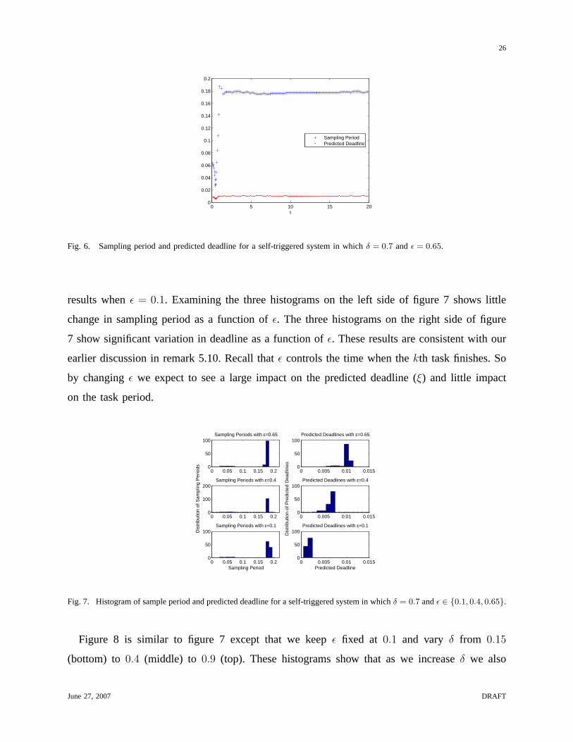
Figure 6 plots the task periods,Tk, (crosses) and deadlines,ξ, (dots) generated by the self-

triggered scheme. The sampling periods range between0.027 to 0.187. This is an order of

magnitude lower than the periods generated by the event-triggered scheme in the preceding

subsection. These sampling periods, however, still show significant variability. The shortest and

most aggressive sampling periods occured in response to the system’s non-zero initial condition.

Longer and relatively constant sampling periods were generated once the system state has

returned to the neighborhood of the system’s equilibrium point. This seems to confirm the

conjecture that self-triggering can effectively adjust task periods in response to changes in the

control system’s external inputs.

Figures 7 and 8 show what happens to task periods and deadlines when we variedδ and

ε. In figure 7, δ = 0.7 and ε was varied between0.1, 0.4 and 0.65. The top two plots show

histograms of the sampling period (left) and deadline (right) forε = 0.65. The middle two plots

are histograms of the sampling periods and deadlines forε = 0.4. The bottom two plots display

June 27, 2007 DRAFT

26

0 5 10 15 200

0.02

0.04

0.06

0.08

0.1

0.12

0.14

0.16

0.18

0.2

t

Sampling PeriodPredicted Deadline

Fig. 6. Sampling period and predicted deadline for a self-triggered system in whichδ = 0.7 and ε = 0.65.

results whenε = 0.1. Examining the three histograms on the left side of figure 7 shows little

change in sampling period as a function ofε. The three histograms on the right side of figure

7 show significant variation in deadline as a function ofε. These results are consistent with our

earlier discussion in remark 5.10. Recall thatε controls the time when thekth task finishes. So

by changingε we expect to see a large impact on the predicted deadline (ξ) and little impact

on the task period.

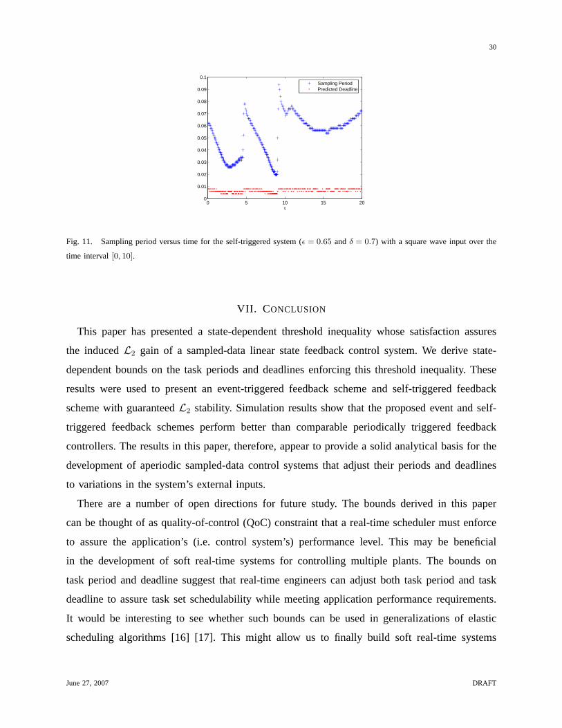
0 0.05 0.1 0.15 0.20

50

100Sampling Periods with ε=0.65

0 0.005 0.01 0.0150

50

100Predicted Deadlines with ε=0.65

0 0.05 0.1 0.15 0.20

100

200

Dis

trib

utio

n of

Sam

plin

g P

erio

ds

Sampling Periods with ε=0.4

0 0.005 0.01 0.0150

50

100

Dis

trib

utio

n of

Pre

dict

ed D

eadl

ines

Predicted Deadlines with ε=0.4

0 0.05 0.1 0.15 0.20

50

100

Sampling Period

Sampling Periods with ε=0.1

0 0.005 0.01 0.0150

50

100

Predicted Deadline

Predicted Deadlines with ε=0.1

Fig. 7. Histogram of sample period and predicted deadline for a self-triggered system in whichδ = 0.7 andε ∈ {0.1, 0.4, 0.65}.

Figure 8 is similar to figure 7 except that we keepε fixed at 0.1 and vary δ from 0.15

(bottom) to 0.4 (middle) to 0.9 (top). These histograms show that as we increaseδ we also

June 27, 2007 DRAFT

27

enlarge the task periods. Recall thatδ controls the time intervalfk+1 − fk so that what we

observe in the simulation is again consistent with our comments in remark 5.9. As we increase

the sampling period, however, we can expect smaller predicted deadlines because the average

sampling frequency is lower. This too is seen in the histograms on the righthand side of figure

8.

0 0.05 0.1 0.15 0.20

50Sampling Periods with δ=0.9

0 0.005 0.01 0.015 0.020

50

100Predicted Deadlines with δ=0.9

0 0.05 0.1 0.15 0.20

50

100Sampling Periods with δ=0.4

Dis

trib

utio

n of

Sam

plin

g P

erio

ds

0 0.005 0.01 0.015 0.020

100

200Predicted Deadlines with δ=0.4

Dis

trib

utio

n of

Pre

dict

ed D

eadl

ines

0 0.05 0.1 0.15 0.20

100

200Sampling Periods with δ=0.15

Sampling Period0 0.005 0.01 0.015 0.02

0

100

200Predicted Deadlines with δ=0.15

Predicted Deadline

Fig. 8. Histogram of sample period and predicted deadline for a self-triggered system in whichε = 0.1 andδ ∈ {0.15, 0.40.9}.

The results in this subsection clearly show that we can effectively bound the task periods and

deadlines in a way that preserves the closed loop system’sL2 stability. An interesting future

research topic concerns how we might use these bounds on period and deadline in a systematic

manner to schedule multiple real-time control tasks.

C. Self-triggered versus Periodically Triggered Control

The simulations in this subsection directly compare the performance of self-triggered and

”comparable” periodically triggered feedback control systems. These simulations were done

on the inverted pendulum system described above. The self-triggered simulations assumed that

ε = 0.65 andδ = 0.7 and task delays were set equal to the deadlines given by the functionξ.

The state trajectories were compared against periodically triggered systems with acomparable

task period and delays. The comparable task periods were chosen from the sample periods

generated by a self-triggered system whose exogenous inputs were chosen to be a noise process

in which ‖w(t)‖2 ≤ 0.01‖x(t)‖2. The delay was set equal to the minimum predicted deadline.

June 27, 2007 DRAFT

28

Figure 9 plots the sample periods,Tk, and predicted deadlines generated by such a self-triggered

system. After the initial transient in response to the system’s non-zero initial condition, the

sampling periods converge onto a periodic signal in which the sample periods range between

0.055 to 0.104. The mean sample period over the interval when the system is near its equilibrium

point is taken as the ”comparable” period for a periodically triggered control system. This

comparable period was0.0673. The comparable delay was set to the minimum predicted deadline

which was0.004.

0 5 10 15 20 25 30 35 400

0.02

0.04

0.06

0.08

0.1

0.12

t

Sampling PeriodPredicted Deadline

Fig. 9. Sample periods generated by a self-triggered system (ε = 0.65 andδ = 0.7) driven by a noise process.

It is interesting to note thatTk shows significant periodic variation in figure 9. Other sim-

ulations have shown similar results. These observations suggest that the choice of ”optimal”

sampling period has its own dynamic that leads to a period variation in the sampling periods.

One interesting issue for future research is whether or not we can take advantage of this variability

in the scheduling of multiple real-time control tasks.

We compared the self-triggered and periodically triggered system’s performance by examining

their normalized state errors,E(t), given by

E(t) =|V (x(t))− V (xc(t))|

V (xc(t))

where V (x) = xT Px and P is the positive definite matrix satisfying the algebraic Riccati

equation 2. This normalization of the state error allows us to fairly compare those states (i.e. the

pendulum bob angle) that are most directly affected by input disturbances. The results from this

comparison are shown in figure 10. This figure plots the time history of the normalized error,

June 27, 2007 DRAFT

29

E(t), for the inverted pendulum using the input signal,w(t) = µ(t) + ν(t) whereν is a white

noise process such that‖ν(t)‖2 ≤ 0.01‖x(t)‖2 andµ : < → < takes the values

µ(t) =

sgn(sin(0.7t)) if 0 ≤ t < 10

0 otherwise.

The functionµ is a square wave input to the system that we’ll use to see how the self-triggered

and periodically triggered systems react to external disturbances. The figure plots the normalized

error for the self-triggered system and a comparable periodically triggered system. As noted

above the period for the periodically-triggered system was chosen from the ”steady-state” sample

periods generated by the self-triggered system (see figure 9).

0 5 10 15 200

0.01

0.02

0.03

0.04

0.05

0.06

0.07

t

E(t) for self−triggered systemE(t) for periodically triggered system

Fig. 10. Normalized error,E(t), versus time for a self-triggered system (ε = .65 and δ = 0.7) and a periodically triggered

system whose period was chosen from the sample periods shown in figure 9.

Figure 10 clearly shows that the self-triggered error is significantly smaller than the error of

the periodically triggered system. This error is a direct result of the self-triggered system’s ability

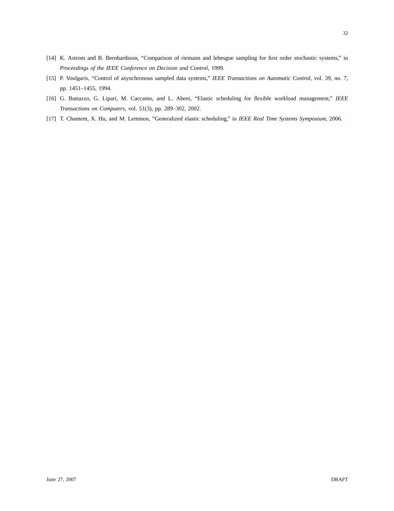
to adjust its sample period. Figure 11 plots the sampling periods generated by the self-triggered

system for the preceding system. This plot shows that the sampling period readjusts and gets

smaller when the square wave input hits the system over the time interval[0, 10]. These results

again demonstrate the ability of self-triggering to successfully adapt to changes in the system’s

input disturbances.

June 27, 2007 DRAFT

30

0 5 10 15 200

0.01

0.02

0.03

0.04

0.05

0.06

0.07

0.08

0.09

0.1

t

Sampling PeriodPredicted Deadline

Fig. 11. Sampling period versus time for the self-triggered system (ε = 0.65 andδ = 0.7) with a square wave input over the

time interval[0, 10].

VII. C ONCLUSION

This paper has presented a state-dependent threshold inequality whose satisfaction assures

the inducedL2 gain of a sampled-data linear state feedback control system. We derive state-

dependent bounds on the task periods and deadlines enforcing this threshold inequality. These

results were used to present an event-triggered feedback scheme and self-triggered feedback

scheme with guaranteedL2 stability. Simulation results show that the proposed event and self-

triggered feedback schemes perform better than comparable periodically triggered feedback

controllers. The results in this paper, therefore, appear to provide a solid analytical basis for the

development of aperiodic sampled-data control systems that adjust their periods and deadlines

to variations in the system’s external inputs.

There are a number of open directions for future study. The bounds derived in this paper

can be thought of as quality-of-control (QoC) constraint that a real-time scheduler must enforce

to assure the application’s (i.e. control system’s) performance level. This may be beneficial

in the development of soft real-time systems for controlling multiple plants. The bounds on

task period and deadline suggest that real-time engineers can adjust both task period and task

deadline to assure task set schedulability while meeting application performance requirements.

It would be interesting to see whether such bounds can be used in generalizations of elastic

scheduling algorithms [16] [17]. This might allow us to finally build soft real-time systems

June 27, 2007 DRAFT

31

providing guarantees on application performance that have traditionally been found only in hard

real-time control systems.

To our best knowledge, this is the first rigorous examination of what might be required to

implement self-triggered feedback control systems. Self-triggering on single processor systems

may not be very useful since event-triggers can often be implemented in an inexpensive manner

using programmable gate arrays (FPGA) or custom analog integrated circuits (ASIC). If, however,

we are controlling multiple plants over a wireless network, then the inability of such networks

to provide deterministic guarantees on message delivery make the use of self-triggered feedback

much more attractive. An interesting future research direction would explore the use of self-

triggered feedback over wireless sensor-actuator networks.

REFERENCES

[1] M. Lemmon, T. Chantem, X. Hu, and M. Zyskowski, “On self-triggered full information h-infinity controllers,” inHybrid

Systems: computation and control, 2007.

[2] M. Velasco, P. Marti, and J. Fuertes, “The self triggered task model for real-time control systems,” inWork-in-Progress

Session of the 24th IEEE Real-Time Systems Symposium (RTSS03), 2003.

[3] K. Astrom and B. Wittenmark,Computer-Controlled Systems: theory and design, 2nd ed. Prentice-Hall, 1990.

[4] Y. Zheng, D. Owens, and S. Billings, “Fast sampling and stability of nonlinear sampled-data systems: Part 2. sampling

rate estimations,”IMA Journal of Mathematical Control and Information, vol. 7, pp. 13–33, 1990.

[5] D. Nesic, A. Teel, and E. Sontag, “Formulas relating kl stability estimates of discrete-time and sampled-data nonlinear

systems,”Systems and Control Letters, vol. 38, pp. 49–60, 1999.

[6] P. Tabuada and X. Wang, “Preliminary results on state-triggered scheduling of stabilizing control tasks,” inIEEE Conference

on Decision and Control, 2006.

[7] D. Seto, J. Lehoczky, L. Sha, and K. Shin, “On task schedulability in real-time control systems,” inIEEE Real-time

Technology and Applications Symposium (RTAS), 1996, pp. 13–21.

[8] A. Cervin, J. Eker, B. Bernhardsson, and K.-E. Arzen, “Feedback-feedforward scheduling of control tasks,”Real-time

Systems, vol. 23(1-2), pp. 25–53, 2002.

[9] P. Marti, C. Lin, S. Brandt, M. Velasco, and J. Fuertes, “Optimal state feedback resource allocation for resource-constrained

control tasks,” inIEEE Real-Time Systems Symposium (RTSS 2004), 2004, p. 161172.

[10] B. Bamieh, “Intersample and finite wordlength effects in sampled-data problems,”IEEE Transactions on Automatic Control,

vol. 48, no. 4, pp. 639–643, 2003.

[11] C. Liu and J. Layland, “Scheduling for multiprogramming in a hard-real-time environment,”Journal of the Association

for Computing Machinery, vol. 20, no. 1, pp. 46–61, 1973.

[12] K. Arzen, “A simple event-based PID controller,” inProceedings of the 14th IFAC World Congress, 1999.

[13] D. Hristu-Varsakelis and P. Kumar, “Interrupt-based feedback control over a shared communication medium,” in

Proceedings of the IEEE Conference on Decision and Control, 2002.

June 27, 2007 DRAFT

32

[14] K. Astrom and B. Bernhardsson, “Comparison of riemann and lebesgue sampling for first order stochastic systems,” in

Proceedings of the IEEE Conference on Decision and Control, 1999.

[15] P. Voulgaris, “Control of asynchronous sampled data systems,”IEEE Transactions on Automatic Control, vol. 39, no. 7,

pp. 1451–1455, 1994.

[16] G. Buttazzo, G. Lipari, M. Caccamo, and L. Abeni, “Elastic scheduling for flexible workload management,”IEEE

Transactions on Computers, vol. 51(3), pp. 289–302, 2002.

[17] T. Chantem, X. Hu, and M. Lemmon, “Generalized elastic scheduling,” inIEEE Real Time Systems Symposium, 2006.

June 27, 2007 DRAFT