1

Salt-and-Pepper Noise Removal by

Median-type Noise Detectors and

Detail-preserving RegularizationRaymond H. Chan, Chung-Wa Ho, and Mila Nikolova

Abstract

This paper proposes a two-phase scheme for removing salt-and-pepper impulse noise. In the first

phase, an adaptive median filter is used to identify pixels which are likely to be contaminated by noise

(noise candidates). In the second phase, the image is restored using a specialized regularization method

that applies only to those selected noise candidates. In terms of edge preservation and noise suppression,

our restored images show a significant improvement compared to those restored by using just nonlinear

filters or regularization methods only. Our scheme can remove salt-and-pepper-noise with noise level as

high as 90%.

Index Terms

Impulse noise, adaptive median filter, edge-preserving regularization.

I. I NTRODUCTION

Impulse noise is caused by malfunctioning pixels in camera sensors, faulty memory locations in

hardware, or transmission in a noisy channel. See [5] for instance. Two common types of impulse noise

are the salt-and-pepper noise and the random-valued noise. For images corrupted by salt-and-pepper

noise (respectively random-valued noise), the noisy pixels can take only the maximum and the minimum

R. H. Chan and C. W. Ho are with the Department of Mathematics, The Chinese University of Hong Kong, Shatin, Hong

Kong (email: rchan, cwho@math.cuhk.edu.hk). This work was supported by HKRGC Grant CUHK4243/01P and CUHK DAG

2060220.

M. Nikolova is with the Centre de Mathematiques et de Leurs Applications, ENS de Cachan, 61 av. du President Wilson,

94235 Cachan Cedex (email: nikolova@cmla.ens-cachan.fr)

July 30, 2004 DRAFT

2

values (respectively any random value) in the dynamic range. There are many works on the restoration

of images corrupted by impulse noise. See, for instance, the nonlinear digital filters reviewed in [1]. The

median filter was once the most popular nonlinear filter for removing impulse noise, because of its good

denoising power [5] and computational efficiency [16]. However, when the noise level is over 50%, some

details and edges of the original image are smeared by the filter [20].

Different remedies of the median filter have been proposed, e.g. the adaptive median filter [17], the

multi-state median filter [11], or the median filter based on homogeneity information [12], [21]. These

so-called “decision-based” or “ switching” filters first identify possible noisy pixels and then replace them

by using the median filter or its variants, while leaving all other pixels unchanged. These filters are good

at detectingnoise even at a high noise level. Their main drawback is that the noisy pixels are replaced

by some median value in their vicinity without taking into account local features such as the possible

presence of edges. Hence details and edges are not recovered satisfactorily, especially when the noise

level is high.

For images corrupted by Gaussian noise, least-squares methods based on edge-preserving regularization

functionals [4], [9], [10], [22] have been used successfully to preserve the edges and the details in the

images. These methods fail in the presence of impulse noise because the noise is heavy tailed. Moreover

the restoration will alter basically all pixels in the image, including those that are not corrupted by

the impulse noise. Recently, non-smooth data-fidelity terms (e.g.`1) have been used along with edge-

preserving regularization to deal with impulse noise [19].

In this paper, we propose a powerful two-stage scheme which combines the variational method proposed

in [19] with the adaptive median filter [17]. More precisely, the noise candidates are first identified by the

adaptive median filter, and then these noise candidates are selectively restored using an objective function

with an `1 data-fidelity term and an edge-preserving regularization term. Since the edges are preserved

for the noise candidates, and no changes are made to the other pixels, the performance of our combined

approach is much better than that of either one of the methods. Salt-and-pepper noise with noise ratio

as high as 90% can be cleaned quite efficiently.

The outline of the paper is as follows. The adaptive median filter and the edge-preserving method

are reviewed in Section II. Our denoising scheme is presented in Section III. Experimental results and

conclusions are presented in Sections IV and V, respectively.

July 30, 2004 DRAFT

3

II. A DAPTIVE MEDIAN FILTER AND EDGE-PRESERVING REGULARIZATION

A. Review of the adaptive median filter

Let xi,j , for (i, j) ∈ A ≡ {1, . . . , M} × {1, . . . , N}, be the gray level of a trueM -by-N imagex at

pixel location(i, j), and[smin, smax] be the dynamic range ofx, i.e.smin ≤ xi,j ≤ smax for all (i, j) ∈ A.

Denote byy a noisy image. In the classical salt-and-pepper impulse noise model, the observed gray level

at pixel location(i, j) is given by

yi,j =

smin, with probability p,

smax, with probability q,

xi,j , with probability 1− p− q,

wherer = p + q defines the noise level. Here we give a brief review of the filter.

Let Swi,j be a window of sizew × w centered at(i, j), i.e.

Swi,j = {(k, l) : |k − i| ≤ w and |j − l| ≤ w}

and letwmax×wmax be the maximum window size. The algorithm tries to identify the noise candidates

yi,j , and then replace eachyi,j by the median of the pixels inSwi,j .

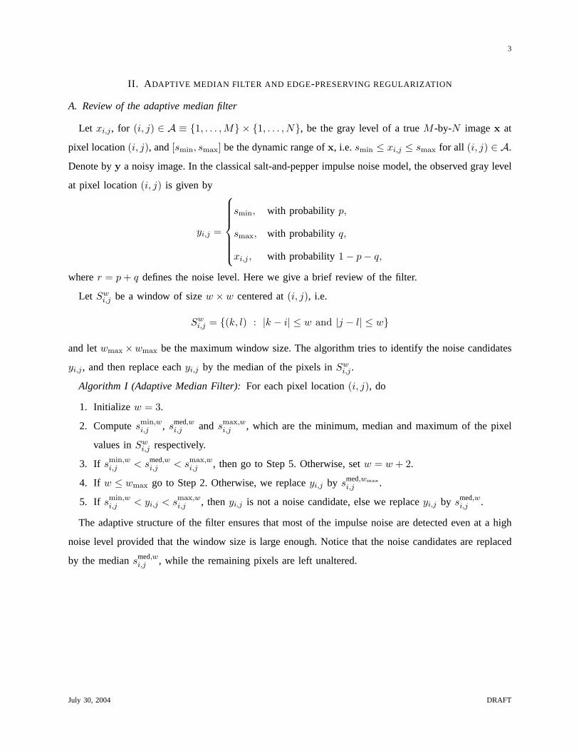
Algorithm I (Adaptive Median Filter):For each pixel location(i, j), do

1. Initialize w = 3.

2. Computesmin,wi,j , smed,w

i,j and smax,wi,j , which are the minimum, median and maximum of the pixel

values inSwi,j respectively.

3. If smin,wi,j < smed,w

i,j < smax,wi,j , then go to Step 5. Otherwise, setw = w + 2.

4. If w ≤ wmax go to Step 2. Otherwise, we replaceyi,j by smed,wmax

i,j .

5. If smin,wi,j < yi,j < smax,w

i,j , thenyi,j is not a noise candidate, else we replaceyi,j by smed,wi,j .

The adaptive structure of the filter ensures that most of the impulse noise are detected even at a high

noise level provided that the window size is large enough. Notice that the noise candidates are replaced

by the mediansmed,wi,j , while the remaining pixels are left unaltered.

July 30, 2004 DRAFT

4

B. Variational method for impulse noise cleaning

In [19], images corrupted by impulse noise are restored by minimizing a convex objective function

Fy : RM×N → R of the form

Fy(u) =∑

(i,j)∈A|ui,j − yi,j |

+β

2

∑

(i,j)∈A

∑

(m,n)∈Vi,j

ϕ(ui,j − um,n), (1)

whereVi,j is the set of the four closest neighbors of(i, j), not including(i, j). It was shown in [18] and

[19] that under mild assumptions and a pertinent choice ofβ, the minimizeru of Fy satisfiesui,j = yi,j

for most of the uncorrupted pixelsyi,j . Furthermore, all pixelsui,j such thatui,j 6= yi,j are restored so

that edges and local features are well preserved, provided thatϕ is an edge-preserving potential function.

Examples of such functions are:

ϕ(t) =√

α + t2, α > 0,

ϕ(t) = |t|α, 1 < α ≤ 2,

see [3], [4], [10], [14]. The minimization algorithm works on the residualsz = u − y. It is sketched

below:

Algorithm II:

1. Initialize z(0)ij = 0 for each(i, j) ∈ A.

2. At each iterationk, calculate, for each(i, j) ∈ A,

ξ(k)i,j = β

∑

(m,n)∈Vi,j

ϕ′(yi,j − zm,n − ym,n),

wherezm,n, for (m,n) ∈ Vi,j , are the latest updates andϕ′ is the derivative ofϕ.

3. If∣∣ξ(k)

i,j

∣∣ ≤ 1, setz(k)i,j = 0. Otherwise, solve forz(k)

i,j in the nonlinear equation

β∑

(m,n)∈Vi,j

ϕ′(z(k)i,j + yi,j − zm,n − ym,n) = sign(ξ(k)

i,j ). (2)

The updating ofz(k)i,j can be done in a red-black fashion, and it was shown in [19] thatz(k) converges

to z = u− y, where the restored imageu minimizesFy in (1). If we chooseϕ(t) = |t|α, the nonlinear

equation (2) can be solved by Newton’s method with quadratic convergence by using a suitable initial

guess derived in [6].

July 30, 2004 DRAFT

5

III. O UR METHOD

Many denoising schemes are “decision-based” median filters, see for example, [11], [12], [24]. This

means that the noise candidates are first detected by some rules and are replaced by the median output

or its variants. For instance, in Algorithm I, the noise candidateyi,j , (i, j) ∈ N , is replaced bysmed,wi,j .

These schemes are good because the uncorrupted pixels will not be modified. However, the replacement

methods in these denoising schemes cannot preserve the features of the images, in particular the edges

are smeared.

In contrast, Algorithm II can preserve edges during denoising but it has problem in detecting noisy

patches, i.e., a connected region containing many noisy pixels. If one wishes to smooth out all the noisy

patches, one has to increaseβ, see [7] for the role ofβ. As a result, the values of some pixels near edges

will be distorted.

Combining both methods will avoid the drawbacks of either one of them. The aims of our method are

to correct noisy pixels and preserve edges in the image. In the following, we denote the restored image

by x.

Algorithm III:

1. (Noise detection):Denote byy the image obtained by applying an adaptive median filter to the

noisy imagey. Noticing that noisy pixels take their values in the set{smin, smax}, we define the

noise candidate set as

N = {(i, j) ∈ A : yi,j 6= yi,j andyi,j ∈ {smin, smax}} .

The set of all uncorrupted pixels isN c = A \ N .

2. (Replacement):Since all pixels inN c are detected as uncorrupted, we naturally keep their original

values, i.e.,xi,j = yi,j for all (i, j) ∈ N c. Let us now consider a noise candidate, say, at(i, j) ∈ N .

Each one of its neighbors(m,n) ∈ Vi,j is either a correct pixel, i.e.,(m,n) ∈ N c and hence

xm,n = ym,n; or is another noise candidate, i.e.,(m,n) ∈ N , in which case its value must be

restored. The neighborhoodVi,j of (i, j) is thus split asVi,j = (Vi,j ∩ N c) ∪ (Vi,j ∩ N ). Noise

candidates are restored by minimizing a functional of the form (1), but restricted to the noise

candidate setN :

Fy

∣∣N (u) =

∑

(i,j)∈N

[|ui,j − yi,j |+ β

2(S1 + S2)

](3)

July 30, 2004 DRAFT

6

where

S1 =∑

(m,n)∈Vi,j∩N c

2 · ϕ(ui,j − ym,n),

S2 =∑

(m,n)∈Vi,j∩Nϕ(ui,j − um,n).

The restored imagex with indices(i, j) ∈ N is the minimizer of (3) which can be obtained by

using Algorithm II but restricted ontoN instead of ontoA. As in (1), the`1 data-fidelity term

|ui,j − yi,j | discourages those wrongly detected uncorrupted pixels inN from being modified to

other values. The regularization term(S1 +S2) performs edge-preserving smoothing for the pixels

indexed byN .

Let us emphasize that Step 1 of our method can be realized by any reliable impulse noise detector,

such as the multi-state median filter [11] or the improved detector [24], etc. Our choice, the adaptive

median filter, was motivated by the fact that it provides a good compromise between simplicity and robust

noise detection, especially for high level noise ratios. The pertinence of this choice can be seen from the

experimental results in [13] (where the noise level is 50%) or Figures 3(h) and 4(h) (where the noise

level is 70%).

IV. SIMULATIONS

A. Configuration

Among the commonly tested 512-by-512 8-bit gray-scale images, the one with homogeneous region

(Lena) and the one with high activity (Bridge) will be selected for our simulations. Their dynamic ranges

are [0, 255]. In the simulations, images will be corrupted by “salt” (with value 255) and “pepper” (with

value 0) noise with equal probability. Also a wide range of noise levels varied from 10% to 70% with

increments of 10% will be tested. Restoration performances are quantitatively measured by the peak

signal-to-noise ratio (PSNR) and the mean absolute error (MAE) defined in [5, p. 327]:

PSNR = 10 log10

2552

1MN

∑i,j(ri,j − xi,j)2

,

MAE =1

MN

∑

i,j

|ri,j − xi,j |,

whereri,j andxi,j denote the pixel values of the restored image and the original image, respectively.

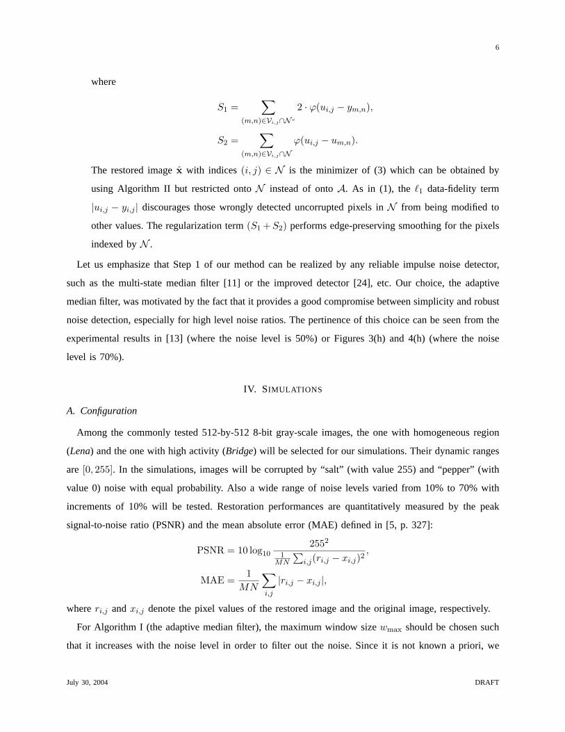
For Algorithm I (the adaptive median filter), the maximum window sizewmax should be chosen such

that it increases with the noise level in order to filter out the noise. Since it is not known a priori, we

July 30, 2004 DRAFT

7

TABLE I

MAXIMUM WINDOW SIZE wmax IN ALGORITHM I.

noise level wmax × wmax

r < 25% 5× 5

25% ≤ r < 40% 7× 7

40% ≤ r < 60% 9× 9

60% ≤ r < 70% 13× 13

70% ≤ r < 80% 17× 17

80% ≤ r < 85% 25× 25

85% ≤ r ≤ 90% 39× 39

tried differentwmax for any given noise level, and found thatwmax given in Table I are sufficient for the

filtering. We therefore setwmax = 39 in all our tests. We remark that with such choice ofwmax, almost

all the salt-and-pepper noise are detected in the filtered images.

For Algorithm II (the variational method in [19]), we chooseϕ(t) = |t|α as the edge-preserving

function. We observe that ifα is small (1 < α < 1.1), most of the noise is suppressed but staircases

appear. Ifα is large (α > 1.5), the fine details are not distorted seriously but the noise cannot be fully

suppressed. The selection ofα is a trade-off between noise suppression and detail preservation [19]. In

the tests, the best restoration results are not sensitive toα when it is between 1.2 and 1.4. We therefore

chooseϕ(t) = |t|1.3, andβ is tuned to give the best result in terms of PSNR.

For our proposed Algorithm III, the noise candidate setN should be obtained such that most of the

noise are detected. This again amounts to the selection ofwmax. As mentioned,wmax = 39 can be fixed

for most purposes. Then we can restore those noise pixelsyi,j with (i, j) ∈ N . As in Algorithm II, the

edge-preserving functionϕ(t) = |t|1.3 will be used. That leaves only the parameterβ to be determined.

Later, we will demonstrate that our proposed algorithm is very robust with respect toβ and thus we fix

β = 5 in all the tests.

For comparison purpose, Algorithm I, Algorithm II, the standard median (MED) filter, and also recently

proposed filters like the progressive switching median (PSM) filter [23], the multi-state median (MSM)

filter [11], the noise adaptive soft-switching median (NASM) filter [12], the directional difference-based

switching median (DDBSM) filter [15], and the improved switching median (ISM) filter [24] are also

tested. For MED filter, the window sizes are chosen for each noise level to achieve its best performance.

For MSM filter, the maximum center weights of 7, 5 and 3 are tested for each noise level. For ISM filter,

July 30, 2004 DRAFT

8

10 20 30 40 50 60 7015

20

25

30

35

40

45Lena

Noise level (%)

PS

NR

(dB

)

MEDPSMMSMNASMDDBSMISMAlgorithm IAlgorithm IIAlgorithm III

(a)

10 20 30 40 50 60 700

2

4

6

8

10

12

14

16

18Lena

Noise level (%)

MA

E

MEDPSMMSMNASMDDBSMISMAlgorithm IAlgorithm IIAlgorithm III

(b)

Fig. 1. Results in PSNR and MAE for theLena image at various noise levels for different algorithms.

the convolution kernelsK5, K7 andK9 and filtering window sizes of9× 9 and11× 11 are used. The

decision thresholds in PSM, MSM, DDBSM, ISM filters are also tuned to give the best performance in

terms of PSNR.

B. Denoising Performance

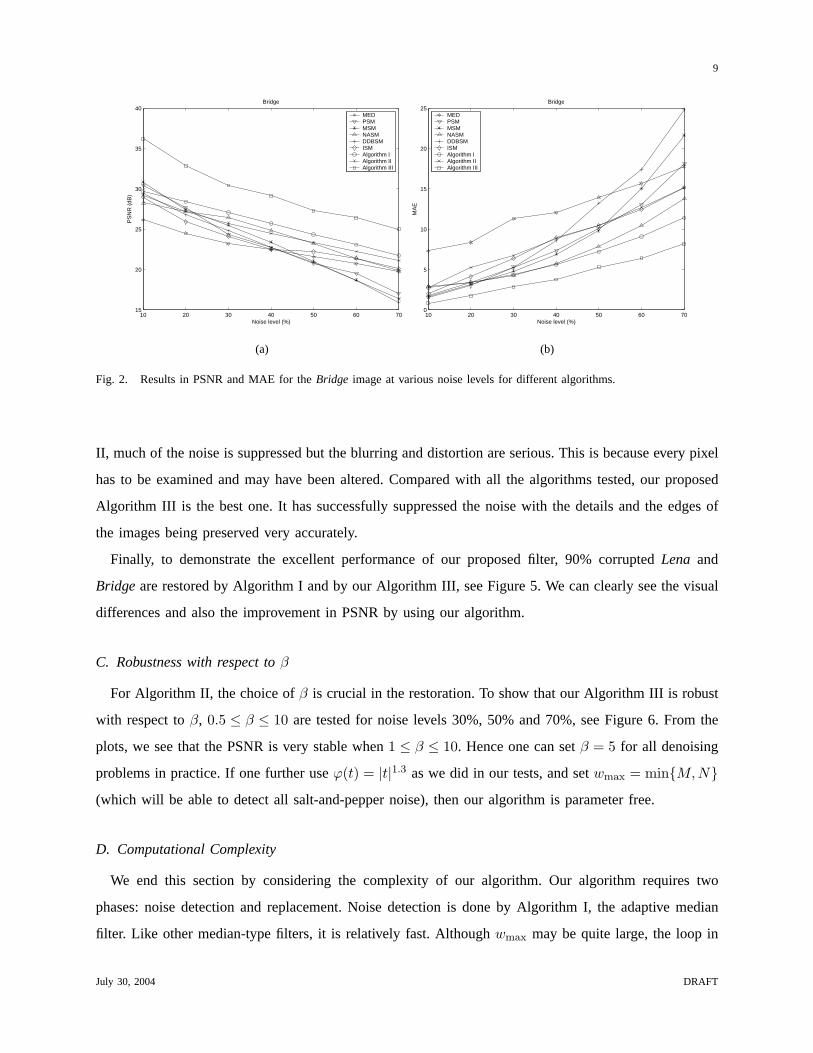
We summarize the performance of different methods in Figures 1 and 2. From the plots, we see that

all the methods have similar performance when the noise level is low. This is because those recently

proposed methods focus on the noise detection. However when the noise level increases, noise patches

will be formed and they may be considered as noise free pixels. This causes difficulties in the noise

detection algorithm. With erroneous noise detection, no further modifications will be made to the noise

patches, and hence their results are not satisfactory.

On the other hand, our proposed denoising scheme achieves a significantly high PSNR and low MAE

even when the noise level is high. This is mainly based on the accurate noise detection by the adaptive

median filter and the edge-preserving property of the variational method of [19].

In Figures 3 and 4, we present restoration results for the 70% corruptedLena and Bridge images.

Among the restorations, except for our proposed one, Algorithm I gives the best performance in terms

of noise suppression and details preservation. As mentioned before, it is because the algorithm locates

the noise accurately. In fact, about 70.2% and 70.4% pixels are detected as noise candidates inLenaand

Bridge respectively by Algorithm I. However, the edges are jittered by the median filter. For Algorithm

July 30, 2004 DRAFT

9

10 20 30 40 50 60 7015

20

25

30

35

40Bridge

Noise level (%)

PS

NR

(dB

)

MEDPSMMSMNASMDDBSMISMAlgorithm IAlgorithm IIAlgorithm III

(a)

10 20 30 40 50 60 700

5

10

15

20

25Bridge

Noise level (%)

MA

E

MEDPSMMSMNASMDDBSMISMAlgorithm IAlgorithm IIAlgorithm III

(b)

Fig. 2. Results in PSNR and MAE for theBridge image at various noise levels for different algorithms.

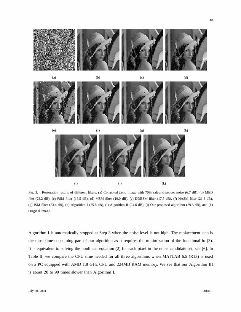
II, much of the noise is suppressed but the blurring and distortion are serious. This is because every pixel

has to be examined and may have been altered. Compared with all the algorithms tested, our proposed

Algorithm III is the best one. It has successfully suppressed the noise with the details and the edges of

the images being preserved very accurately.

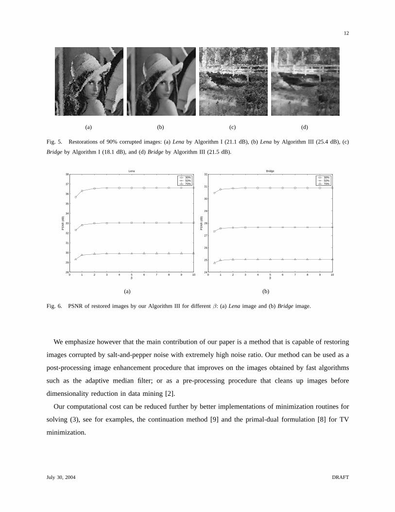
Finally, to demonstrate the excellent performance of our proposed filter, 90% corruptedLena and

Bridge are restored by Algorithm I and by our Algorithm III, see Figure 5. We can clearly see the visual

differences and also the improvement in PSNR by using our algorithm.

C. Robustness with respect toβ

For Algorithm II, the choice ofβ is crucial in the restoration. To show that our Algorithm III is robust

with respect toβ, 0.5 ≤ β ≤ 10 are tested for noise levels 30%, 50% and 70%, see Figure 6. From the

plots, we see that the PSNR is very stable when1 ≤ β ≤ 10. Hence one can setβ = 5 for all denoising

problems in practice. If one further useϕ(t) = |t|1.3 as we did in our tests, and setwmax = min{M,N}(which will be able to detect all salt-and-pepper noise), then our algorithm is parameter free.

D. Computational Complexity

We end this section by considering the complexity of our algorithm. Our algorithm requires two

phases: noise detection and replacement. Noise detection is done by Algorithm I, the adaptive median

filter. Like other median-type filters, it is relatively fast. Althoughwmax may be quite large, the loop in

July 30, 2004 DRAFT

10

(a) (b) (c) (d)

(e) (f) (g) (h)

(i) (j) (k)

Fig. 3. Restoration results of different filters: (a) CorruptedLena image with 70% salt-and-pepper noise (6.7 dB), (b) MED

filer (23.2 dB), (c) PSM filter (19.5 dB), (d) MSM filter (19.0 dB), (e) DDBSM filter (17.5 dB), (f) NASM filter (21.8 dB),

(g) ISM filter (23.4 dB), (h) Algorithm I (25.8 dB), (i) Algorithm II (24.6 dB), (j) Our proposed algorithm (29.3 dB), and (k)

Original image.

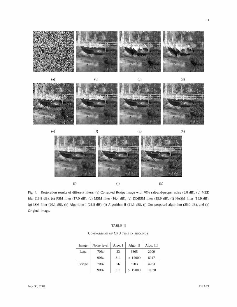
Algorithm I is automatically stopped at Step 3 when the noise level is not high. The replacement step is

the most time-consuming part of our algorithm as it requires the minimization of the functional in (3).

It is equivalent to solving the nonlinear equation (2) for each pixel in the noise candidate set, see [6]. In

Table II, we compare the CPU time needed for all three algorithms when MATLAB 6.5 (R13) is used

on a PC equipped with AMD 1.8 GHz CPU and 224MB RAM memory. We see that our Algorithm III

is about 20 to 90 times slower than Algorithm I.

July 30, 2004 DRAFT

11

(a) (b) (c) (d)

(e) (f) (g) (h)

(i) (j) (k)

Fig. 4. Restoration results of different filters: (a) CorruptedBridge image with 70% salt-and-pepper noise (6.8 dB), (b) MED

filer (19.8 dB), (c) PSM filter (17.0 dB), (d) MSM filter (16.4 dB), (e) DDBSM filter (15.9 dB), (f) NASM filter (19.9 dB),

(g) ISM filter (20.1 dB), (h) Algorithm I (21.8 dB), (i) Algorithm II (21.1 dB), (j) Our proposed algorithm (25.0 dB), and (k)

Original image.

TABLE II

COMPARISON OFCPU TIME IN SECONDS.

Image Noise level Algo. I Algo. II Algo. III

Lena 70% 23 6865 2009

90% 311 > 12000 6917

Bridge 70% 56 8003 4263

90% 311 > 12000 10070

July 30, 2004 DRAFT

12

(a) (b) (c) (d)

Fig. 5. Restorations of 90% corrupted images: (a)Lena by Algorithm I (21.1 dB), (b)Lena by Algorithm III (25.4 dB), (c)

Bridge by Algorithm I (18.1 dB), and (d)Bridge by Algorithm III (21.5 dB).

0 1 2 3 4 5 6 7 8 9 1028

29

30

31

32

33

34

35

36

37

38Lena

β

PS

NR

(dB

)

30%50%70%

(a)

0 1 2 3 4 5 6 7 8 9 1024

25

26

27

28

29

30

31

32Bridge

β

PS

NR

(dB

)

30%50%70%

(b)

Fig. 6. PSNR of restored images by our Algorithm III for differentβ: (a) Lena image and (b)Bridge image.

We emphasize however that the main contribution of our paper is a method that is capable of restoring

images corrupted by salt-and-pepper noise with extremely high noise ratio. Our method can be used as a

post-processing image enhancement procedure that improves on the images obtained by fast algorithms

such as the adaptive median filter; or as a pre-processing procedure that cleans up images before

dimensionality reduction in data mining [2].

Our computational cost can be reduced further by better implementations of minimization routines for

solving (3), see for examples, the continuation method [9] and the primal-dual formulation [8] for TV

minimization.

July 30, 2004 DRAFT

13

V. CONCLUSION

In this paper, we propose a decision-based, details preserving restoration method. It is the ultimate

filter for removing salt-and-pepper noise. Experimental results show that our method performs much

better than median-based filters or the edge-preserving regularization methods. Even at a very high noise

level (≤ 90%), the texture, details and edges are preserved accurately. One can further improve our

results by using different noise detectors and regularization functionals that are tailored to different types

of noises, such as the random-valued impulse noise or impulse-plus-Gaussian noise. These extensions

together with fast solvers for (3) will be given in our forthcoming papers.

REFERENCES

[1] J. Astola and P. Kuosmanen,Fundamentals of Nonlinear Digital Filtering.Boca Raton, CRC, 1997.

[2] E. Bingham and H. Mannila, “Random projection in dimensionality reduction: applications to image and text data,”

Proceedings of the 7th ACM SIGKDD International Conference on Knowledge Discovery and Data Mining (KDD-2001),

August 26-29, 2001, San Francisco, CA, USA, pp. 245–250.

[3] M. Black and A. Rangarajan, “On the unification of line processes, outlier rejection, and robust statistics with applications

to early vision,” International Journal of Computer Vision, 19 (1996), pp. 57–91.

[4] C. Bouman and K. Sauer, “On discontinuity-adaptive smoothness priors in computer vision,”IEEE Transactions on Pattern

Analysis and Machine Intelligence, 17 (1995), pp. 576–586.

[5] A. Bovik, Handbook of Image and Video Processing, Academic Press, 2000.

[6] R. H. Chan, C.-W Ho, and M. Nikolova, “Convergence of Newton’s method for a minimization problem in impulse noise

removal”, Journal of Computational Mathematics, 22 (2004), pp. 168–177.

[7] T. F. Chan and S. Esedoglu, “Aspects of total variation regularizedL1 function approximation,” Department of Mathematics,

UCLA, CAM Report (04-07), 2004.

[8] T. F. Chan, G. H. Golub and P. Mulet, “A nonlinear primal-dual method for total variation-based image restoration,”SIAM

Journal on Scientific Computing, 20 (1999), pp. 1964–1977.

[9] T. F. Chan, H. M. Zhou, and R. H. Chan, “A continuation method for total variation denoising problems,”Proceedings

of SPIE Symposium on Advanced Signal Processing: Algorithms, Architectures, and Implementations, ed. F. T. Luk, 2563

(1995), pp. 314–325,

[10] P. Charbonnier, L. Blanc-Feraud, G. Aubert, and M. Barlaud, “Deterministic edge-preserving regularization in computed

imaging,” IEEE Transactions on Image Processing, 6 (1997), pp. 298–311.

[11] T. Chen and H. R. Wu, “Space variant median filters for the restoration of impulse noise corrupted images,”IEEE

Transactions on Circuits and Systems II, 48 (2001), pp. 784–789.

[12] H.-L. Eng and K.-K. Ma, “Noise adaptive soft-switching median filter,”IEEE Transactions on Image Processing, 10 (2001),

pp. 242–251.

[13] R. C. Gonzalez and R. E. Woods,Digital Image Processing Second Edition, Prentice Hall, 2001; andBook Errata Sheet

(July 31, 2003), http://www.imageprocessingbook.com/downloads/erratasheet.htm.

[14] P. J. Green, “Bayesian reconstructions from emission tomography data using a modified EM algorithm,”IEEE Transactions

on Medical Imaging, MI-9 (1990), pp. 84–93.

July 30, 2004 DRAFT

14

[15] Y. Hashimoto, Y. Kajikawa and Y. Nomura, “Directional difference-based switching median filters,”Electronics and

Communications in Japan, 85 (2002), pp. 22–32.

[16] T. S. Huang, G. J. Yang, and G. Y. Tang, “Fast two-dimensional median filtering algorithm,”IEEE Transactions on

Acoustics, Speech, and Signal Processing, 1 (1979), pp. 13–18.

[17] H. Hwang and R. A. Haddad, “Adaptive median filters: new algorithms and results,”IEEE Transactions on Image

Processing, 4 (1995), pp. 499–502.

[18] M. Nikolova, “Minimizers of cost-functions involving nonsmooth data-fidelity terms. Application to the processing of

outliers,” SIAM Journal on Numerical Analysis, 40 (2002), pp. 965–994.

[19] M. Nikolova, “A variational approach to remove outliers and impulse noise,”Journal of Mathematical Imaging and Vision,

20 (2004), pp. 99–120.

[20] T A. Nodes and N. C. Gallagher, Jr. “The output distribution of median type filters,”IEEE Transactions on Communications,

COM-32, 1984.

[21] G. Pok, J.-C. Liu, and A. S. Nair, “Selective removal of impulse noise based on homogeneity level information,”IEEE

Transactions on Image Processing, 12 (2003), pp. 85–92.

[22] C. R. Vogel and M. E. Oman, “Fast, robust total variation-based reconstruction of noisy, blurred images,”IEEE Transactions

on Image Processing, 7 (1998), pp. 813–824.

[23] Z. Wang and D. Zhang, “Progressive switching median filter for the removal of impulse noise from highly corrupted

images,”IEEE Transactions on Circuits and Systems II, 46 (1999), pp. 78–80.

[24] S. Zhang and M. A. Karim, “A new impulse detector for switching median filters,”IEEE Signal Processing Letters, 9

(2002), pp. 360–363.

July 30, 2004 DRAFT