1-s2.0-s0307904x13007683-main

Applied Mathematical Modelling 38 (2014) 3054–3066

Contents lists available at ScienceDirect

Applied Mathematical Modelling

journal homepage: www.elsevier .com/locate /apm

Large deflections of tapered functionally graded beamssubjected to end forces

0307-904X/$ - see front matter � 2013 Elsevier Inc. All rights reserved.http://dx.doi.org/10.1016/j.apm.2013.11.032

⇑ Corresponding author. Tel.: +84 4 3762 8006; fax: +84 4 3762 2039.E-mail addresses: [email protected], [email protected] (D.K. Nguyen).

Nguyen Dinh Kien a,⇑, Buntara Sthenly Gan b

a Department of Solid Mechanics, Institute of Mechanics, Vietnam Academy of Science and Technology, 18 Hoang Quoc Viet, Hanoi, Viet Namb Department of Architecture, College of Engineering, Nihon University, Koriyama, Fukushima-ken 963-8642, Japan

a r t i c l e i n f o a b s t r a c t

Article history:Received 5 June 2012Received in revised form 24 September 2013Accepted 22 November 2013Available online 15 December 2013

Keywords:Functionally graded materialTapered beamFinite element methodLarge deflection

The large deflections of tapered functionally graded beams subjected to end forces arestudied by using the finite element method. The material properties of the beams areassumed to vary through the thickness direction according to a power law distribution.A first order shear deformable beam element employed the exact polynomials tointerpolate the transverse displacement and rotation, is formulated in the context of theco-rotational approach. The large deflection response of the beams is computed by usingthe arc-length control algorithm in combination with the Newton–Raphson iterativemethod. The numerical results show that the formulated element is capable to assessaccurately the response of the beams by using just several elements. A parametric studyis given to examine the influence of the material non-homogeneity, taper ratio as well asthe aspect ratio on the large deflection behaviour of the beams.

� 2013 Elsevier Inc. All rights reserved.

1. Introduction

Functionally graded materials (FGMs), which were invented by Japanese scientists in Sendai in 1984 [1], have receivedmuch attention from researchers. The FGMs are formed by varying percentage of constituents in any desired spacial direc-tion, and as a result the specific physical and mechanical properties of the formed material can be obtained. FGMs are beingused widely as a structural material, and analysis of FGM structures has become an important topic in the field of structuralmechanics. A comprehensive list of publications on the analysis of FGM structures subjected to different loadings is given ina review paper by Birman and Byrd [2], contributions that are most relevant to the present work are discussed below.

Sankar [3] proposed an elasticity solution for FGM beams under static transverse loads by assuming the material prop-erties to vary in the thickness direction by an exponential law.Based on the first order shear deformation beam theory, Cha-kraborty et al. [4] formulated a beam element for analyzing the thermoelastic behaviour of FGM beams by using the exactsolution of the governing differential equations of an FGM Timoshenko beam segment to interpolate the displacements androtation. Using the spectral finite element method, Chakraborty and Gopalakrishnan [5] studied the wave propagationbehaviour of FGM beams under high frequency impulse loading. Kadoli et al. [6] formulated a beam element to investigatethe static behaviour of metal ceramic beams under ambient temperature by adopting the third order shear deformationbeam theory. Taking the warping effect into consideration, Benatta et al. [7] derived an analytical solution to the bendingproblem of a FGM beam. Singh and Li [8] presented a mathematical model for computing the buckling loads of uniformand non-uniform axially FGM columns. Kang and Li [9,10] proposed closed-form solutions for a nonlinear FGM cantileverbeam with the elastic modulus variation in thickness direction under a tip load or a tip moment by deriving an expression

http://crossmark.crossref.org/dialog/?doi=10.1016/j.apm.2013.11.032&domain=pdf

http://dx.doi.org/10.1016/j.apm.2013.11.032

mailto:[email protected]

mailto:[email protected]


http://www.sciencedirect.com/science/journal/0307904X

http://www.elsevier.com/locate/apm

D.K. Nguyen, B.S. Gan / Applied Mathematical Modelling 38 (2014) 3054–3066 3055

for the effective bending rigidity. Lee et al. [11] presented a finite element procedure for computing the post-bucklingresponse of FGM plates under compressive and thermal loads. Huang and Li [12] studied the free vibration of non-uniformcross-section beams made of an axially FGM. Employing the multilayering method, Kutiš et al. [13] presented a finiteelement procedure for modelling a FGM beam with spatial variation of material properties. Also using the finite elementmethod, Alshorbagy et al. [14] investigated the free vibration characteristics of Euler–Bernoulli beams with materialgraduation in both axially and transversally through the beam thickness. Adopting the Ritz method, Wattanasakulponget al. [15] investigated the thermal buckling and elastic vibration of the third-order shear deformable FGM beams. Shahbaet al. [16] computed the natural frequencies and buckling loads of tapered Timoshenko beams composed of axially FGM byusing the exact shape functions of a uniformed homogeneous Timoshenko beam segment to derive the mass and stiffnessmatrices. Aminbaghai et al. [17] studied the free vibration of FGM beams with continuous spatial polynomial variation ofmaterial properties by a fourth order differential equation of the second order beam theory. Using the finite element method,Nguyen et al. [18] studied the dynamic behaviour of non-uniform FGM Timoshenko beams subjected to a variable speedmoving load.

Non-prismatic beams with variable cross section are of great important in engineering because of their ability in optimiz-ing the weight and strength of structures. Analytical methods are often encountered difficulties in analyzing the non-pris-matic beams due to the presence of variable coefficients in the governing differential equations, and a numerical methods isnecessarily employed instead of. In this line of work, Wood and Zienkiewicz [19] computed the large displacement responseof a non-uniform column subjected to an eccentric axial compressive force by using the finite element method. In [20], Cleg-horn and Tabarrok employed the homogeneous solution of a tapered Timoshenko beam segment to formulate the mass andstiffness matrices for computing the vibration characteristics of the beams. Baker [21] used the weight residual method insolving the governing differential equation of a slender tapered cantilever beam under arbitrarily distributed loads. Lee et al.[22] presented a Runge–Kutta based numerical method to solve the governing differential equations of tapered cantileverbeams under large displacements, and then verified the computed results by performing an experiment on a width taperedsteel beam. Brojan et al. [23] developed an exact moment–curvature formula for determining deformed shape of non-pris-matic cantilever beams obeying the generalized Ludwick law under a tip moment. Attarnejad et al. [24] derived the displace-ment functions for studying the free vibration of non-prismatic beams by solving the governing equations of motion of atapered Timoshenko beam element. Shahba et al. [25] introduced the basic displacement functions and then constructedthe shape functions for derivation of an efficient 2D beam element for the free vibration analysis of rotating tapered Timo-shenko beams.

To the authors’ best knowledge, the large deflection of tapered FGM beams subjected to end forces has not been studied inthe literature and this topic will be the subject of investigation by using the finite element method in the present work. Thematerial properties of the beams are assumed to be described by a power law distribution through the beam thickness. Anonlinear beam element based on the first order shear deformation beam theory, employing the polynomials obtained fromthe solution of the governing differential equations of a uniform homogeneous Timoshenko beam segment to interpolate thetransverse displacement and rotation, is formulated in the context of the co-rotational approach. Using the formulated ele-ment, the large deflection response of a cantilever FGM beam with different taper cases is computed with the aid of the arc-length control algorithm in combination with the iterative Newton–Raphson method. Numerical examples are presented toshow the accuracy and efficiency of the proposed element. The influence of the material distribution, taper ratio as well asthe aspect ratio on the large deflections of the beams is numerically investigated in detail.

2. Tapered FGM beams

Consider a tapered FGM beam with length of L. Three following taper cases are considered in the present work

Case A: A ¼ A0 1� a xL

� �, I ¼ I0 1� a x

L

� �Case B: A ¼ A0 1� a x

L

� �, I ¼ I0 1� a x

L

� �3

Case C: A ¼ A0 1� a xL

� �2, I ¼ I0 1� a xL

� �4

where A0; I0 denote the area and moment of inertia of the section at x ¼ 0, respectively; 0 6 a < 1 is the taper ratio. Fig. 1shows the geometry of the three considered cases of the beam in a co-ordinate system, ðx; y; zÞ, where the z axis directs alongthe thickness direction of the beam.

The beam is assumed to be formed from two different materials with volume fractions to be varied according to a powerlaw as

V1 ¼zhþ 1

2

� �k

; V2 ¼ 1� V1; ð1Þ

where the subscript 1 and 2 indicate the material 1 and material 2 – the constituents of the FGM, respectively; k is the non-negative power law exponent, dictating the material variation through the beam thickness; h is the section height, whichlongitudinally varies for the case B and case C. According to the rule of mixture, the effective Young’s modulus E, and theeffective shear modulus G of the FGM beam are given by

Fig. 1. FGM beam with three considered taper cases.

200 250 300 350 400−0.5

−0.25

0

0.25

0.5

E (GPa)

z/h

k = 1

k = 2 k = 3

k = 5

k = 0.2

k = 0.5

80 90 100 110 120 130 140−0.5

−0.25

0

0.25

0.5

G (GPa)

z/h

k = 0.5

k = 0.2

k = 1

k = 2 k = 3

k = 5

Fig. 2. Variation of Young’s and shear moduli through the thickness of FGM beam formed from steel and alumina.

3056 D.K. Nguyen, B.S. Gan / Applied Mathematical Modelling 38 (2014) 3054–3066

EðzÞ ¼ ðE1 � E2Þzhþ 1

2

� �k

þ E2;

GðzÞ ¼ ðG1 � G2Þzhþ 1

2

� �k

þ G2;

ð2Þ

where E1; E2 and G1;G2 denote the Young’s and shear moduli of the constituents. It is evident from Eq. (2) that whenz ¼ �h=2; E ¼ E2;G ¼ G2, and thus the bottom surface contains purely material 2; when z ¼ h=2; E ¼ E1;G ¼ G1, and thetop surface contains only material 1. Fig. 2 shows the variation of the effective Young’s modulus and the shear modulusthrough the thickness of a FGM beam formed from steel and alumina. The Young’s and shear moduli of the alumina and steelare as follows [4]: Ea ¼ 390 GPa, Es ¼ 210 GPa, Ga ¼ 137 GPa, Gs ¼ 80 GPa, where the subscript ‘a’ and ‘s’ stand for ‘alumina’and ‘steel’, respectively.

3. Finite element formulation

3.1. Large deflection analysis

A convenient way to formulate a geometrically nonlinear element is to introduce a local coordinate system which con-tinuously moves and rotates during the element deformation process. The element formulation is firstly derived in the localsystem then transferred into the global one with the aid of transformation matrices defined from the relationship betweenthe local and global nodal displacements. The method is known in the literature as the co-rotational method [26,27], and willbe adopted herein.


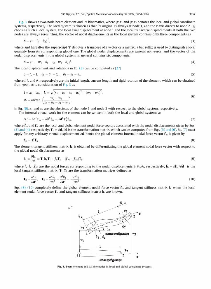
Fig. 3 shows a two-node beam element and its kinematics, where ð�x;�zÞ and ðx; zÞ denotes the local and global coordinatesystems, respectively. The local system is chosen as that its original is always at node 1, and the x axis directs to node 2. Bychoosing such a local system, the local axial displacement at node 1 and the local transverse displacements at both the twonodes are always zeros. Thus, the vector of nodal displacements in the local system contains only three components as

�d ¼ f�u �h1�h2g

T; ð3Þ

where and hereafter the superscript ‘T’ denotes a transpose of a vector or a matrix; a bar suffix is used to distinguish a localquantity from its corresponding global one. The global nodal displacements are general non-zeros, and the vector of thenodal displacements in the global system, in general contains six components

d ¼ fu1 w1 h1 u2 w2 h2gT: ð4Þ

The local displacement and rotations in Eq. (3) can be computed as [27]

�u ¼ ln � l; �h1 ¼ h1 � hr; �h2 ¼ h2 � hr: ð5Þ

where l; ln and hr , respectively are the initial length, current length and rigid rotation of the element, which can be obtainedfrom geometric consideration of Fig. 3 as

l ¼ x2 � x1; ln ¼ffiffiffiffiffiffiffiffiffiffiffiffiffiffiffiffiffiffiffiffiffiffiffiffiffiffiffiffiffiffiffiffiffiffiffiffiffiffiffiffiffiffiffiffiffiffiffiffiffiffiffiffiffiffiffiffiffiffiffiffiffiffiffiffiffiffiffiffiffiffiffiffiðx2 þ u2 � x1 � u1Þ2 þ ðw2 �w1Þ2

q;

hr ¼ arctanw2 �w1

x2 þ u2 � x1 � u1

� �:

ð6Þ

In Eq. (6), x1 and x2 are the abscissas of the node 1 and node 2 with respect to the global system, respectively.The internal virtual work for the element can be written in both the local and global systems as

dU ¼ ddT f in ¼ d�dT �f in ¼ ddT TT1�f in; ð7Þ

where �f in and f in are the local and global element nodal force vectors associated with the nodal displacements given by Eqs.(3) and (4), respectively; T1 ¼ @�d=@d is the transformation matrix, which can be computed from Eqs. (5) and (6). Eq. (7) mustapply for any arbitrary virtual displacement dd, hence the global element internal nodal force vector f in is given by

f in ¼ TT1�f in: ð8Þ

The element tangent stiffness matrix, kt is obtained by differentiating the global element nodal force vector with respect tothe global nodal displacements as

kt ¼@f in

@d¼ TT

1�kt T1 þ �f uT2 þ ð�f h1 þ �f h2ÞT3; ð9Þ

where �f u;�f h1;

�f h2 are the nodal forces corresponding to the nodal displacements �u; �h1; �h2, respectively; �kt ¼ @�f in=@�d is the

local tangent stiffness matrix; T2;T3 are the transformation matrices defined as

T2 ¼@2�u

@d2 ; T3 ¼@2�h1

@d2 ¼@2�h2

@d2 ¼ �@2hr

@d2 : ð10Þ

Eqs. (8)–(10) completely define the global element nodal force vector f in and tangent stiffness matrix kt when the localelement nodal force vector �f in and tangent stiffness matrix �kt are known.

Fig. 3. Beam element and its kinematics in local and global coordinate systems.


3.2. Local formulation

Adopting the first order shear deformation beam theory, the axial and transverse displacements at any point of the beamcan be expressed in the local system as

uð�x;�zÞ ¼ u0ð�xÞ � �zhð�xÞ; wð�x;�zÞ ¼ w0ð�xÞ; ð11Þ

where u0 and w0, respectively are the axial and transverse displacements of the point on the mid-plane, chosen as the ref-erence plane; hð�xÞ is the cross-sectional rotation. The axial strain, �, and the shear strain, c, for the large deflection analysisare deduced from Eq. (11) as

� ¼ u0;�x þ12

w20;�x

� �� zh;�x ¼ �m þ �zv;

c ¼ w0;�x � h;

ð12Þ

where a coma denotes the derivative with respect to the followed variable; �m is the membrane strain, and v ¼ �h;�x is thebeam curvature. It is noted that in the co-rotational method, a linear definition can be used for the local axial strain [26,27],but as the first author has shown in [28] that by adding the nonlinear term 1

2 w20;x, the convergency of the element can be

improved considerably.Assuming the material of the FGM beam obeys the Hook’s law, the axial stress, r, and shear stress, s, associated with the

axial and shear strains in Eq. (12) are given by

r ¼ Eð�zÞ�; s ¼ wGð�zÞc; ð13Þ

where Eð�zÞ;Gð�zÞ are the effective moduli, defined by Eq. (2) with z is replaced by �z; w denotes the shear correction factor,equals to 5/6 for a rectangular section. The virtual work of the internal force for the element can be expressed as

dU ¼Z l

0

ZA

rd�þ sdcð Þ dAd�x; ð14Þ

where d� and dc are the small arbitrary virtual strains; A denotes the cross section area, which longitudinally varies herein. Inorder to express the virtual work in term of the local nodal displacements, interpolation schemes are necessary to introducefor the kinematic variables. Noting that �u1 ¼ �w1 ¼ �w2 ¼ 0, one can write

u0 ¼ Nu�u; w0 ¼ NTw

�h; h ¼ NTh

�h; ð15Þ

where �h ¼ f�h1�h2g

T; Nw and Nh are the matrices of interpolating functions for w0 and h, respectively. Linear and cubic Hermite

polynomials derived purely from mathematical consideration can be employed to interpolate the displacement field of aFGM beam element [14]. The use of exact shape functions for uniform homogeneous beam elements to interpolate the trans-verse displacement and rotation of the tapered FGM Timoshenko beam leads to a beam element with high accuracy [16]. Inthe present work, linear function is adopted for the axial displacement, Nu ¼ �x=l, and the exact polynomials derived byKosmatka [29] as solutions of the governing differential equations for a uniform homogeneous Timoshenko beam elementare used for the transverse displacement and rotation as

Nw ¼l

1þ /

�xl

� �3 � 2þ /2

� ��xl

� �2 þ 1þ /2

� ��xl

� ��xl

� �3 � 1� /2

� ��xl

� �2 � /2

�xl

� �( )

ð16Þ

and

Nh ¼1

1þ /

3 �xl

� �2 � ð4þ /Þ �xl

� �þ ð1þ /Þ

3 �xl

� �2 � ð2� /Þ �xl

� �( )

: ð17Þ

In Eqs. (16) and (17), / is the ratio of the bending stiffness to the shear stiffness as [29]

/ ¼ 12

l2

EhIh

wGhAh

� �ð18Þ

where the subscript ‘h’ designates the value of the parameters in the homogeneous and isotropic uniform beam. It should benoted that if the notation / ¼ EhIh=ðl2wGhAhÞ is used instead of (18), the interpolation functions in Eqs. (16) and (17) resumethe same forms as that formulated by Reddy in [30], and used by Shahba et al. in [16]. Present work uses the area andmoment of inertia of the cross section at the left node of the element as Ah and Ih, and the Young’s and shear moduli ofthe material at the bottom surface of the beam as Eh and Gh, respectively.

Due to the unbalance interpolations adopted for the axial and transverse displacements, the formulated element mightsuffer from the membrane locking [26]. To overcome this problem, it is necessary to replace the membrane strain in Eq. (12)by the ‘effective strain’, defined as [26]


�eff : ¼1l

Z l

0u0;�x þ

12

w20;�x

� �d�x: ð19Þ

Using Eq. (16), we can write the effective strain (19) in the form

�eff : ¼ bu�uþ 12l

�hTZ l

0bwbT

w d�x �h; ð20Þ

where bu ¼ Nu;�x ¼ 1=l, and

bw ¼ Nw;�x ¼1

1þ /

3 �xl

� �2 � ð4þ /Þ �xl

� �þ 1þ /

2

� �3 �x

l

� �2 � ð2� /Þ �xl

� �� /

2

( ): ð21Þ

With the introduction of the effective strain, the virtual work given by Eq. (14) reads

dU ¼Z l

0ðNd�eff : þMdvþ QdcÞd�x; ð22Þ

where, with the aid of Eqs. (15)–(17), the resultants N;M and Q are given by

N ¼ A11�eff: þ A12v ¼ A11�eff: þ A12bTh�h;

M ¼ A12�eff : þ A22v ¼ A12�eff : þ A22bTh�h;

Q ¼ wA33c ¼ wA33ðbTw � NT

h Þ�h:

ð23Þ

In Eq. (23), bh ¼ �Nh;�x; A11;A12;A22 and A33 denote the extensional, coupling, bending and shear rigidities, respectively anddefined as follows

A11;A12;A22ð Þ ¼Z

AEð�zÞ ð1;�z;�z2ÞdA; A33 ¼

ZA

Gð�zÞdA: ð24Þ

The virtual strains and virtual curvature in Eq. (22) can be computed from Eqs. (15) and (20) as

d�eff: ¼ bud�uþ cTwd�h; dv ¼ bT

hd�h; dc ¼ ðbTw � NT

h Þd�h; ð25Þ

where

cw ¼ �eff:;�h ¼1

60ð1þ /2Þ5/ð2þ /Þ ð�h1 � �h2Þ þ 2ð4�h1 � �h2Þ�5/ð2þ /Þ ð�h1 � �h2Þ � 2ð�h1 � 4�h2Þ

( ): ð26Þ

Substituting Eq. (25) into Eq. (22), one gets

dU ¼Z l

0Nbud�uþ NcT

w þMbTh þ QðbT

w � NTh Þ

h id�h

n od�x ð27Þ

So that the components of the local element nodal force vector are given by

�f u ¼Z l

0Nbud�x;

�fh ¼ �f h1�f h2

� �T ¼Z l

0Ncw þMbh þ Qðbw � NhÞ½ �d�x:

ð28Þ

The local tangent stiffness matrix can be divided into sub-matrices as

�kt ¼�kuu

�kuh

�kTuh

�khh

" #; ð29Þ

where, the sub-matrices can be computed from Eq. (28) with the aid of Eqs. (23)–(26) as follows

�kuu ¼ �f u;�u ¼Z l

0A11b2

udx ¼ 1

l2

Z l

0A11d�x;

�kuh ¼ �f u;�h ¼Z l

0buðA11cT

w þ A12bTh Þd�x;

�khh ¼ �f h;�h ¼Z l

0A11cwcT

w þ NDþ 2A12bhcTw þ A22bhbT

h þ wA33ðbw � NhÞ ðbTw � NT

h Þh i

d�x;

ð30Þ


where D is a symmetric matrix with the following form

Table 1Absolut

P�

505

D ¼ cTw;�h ¼

160ð1þ /2Þ

8þ 10/þ 5/2 �ð2þ 10/þ 5/2Þ�ð2þ 10/þ 5/2Þ 8þ 10/þ 5/2

" #: ð31Þ

The terms containing cw and N in Eq. (30) stemming from the nonlinear part of the local strain, 12 w2

0;�x, and they are functionsof the current local nodal displacements. Eqs. (28) and (30) together with Eqs. (8)–(10) completely define the elementformulation. In order to improve convergency of the numerical result, the rigidities A11;A12;A22 and A33 in the local elementnodal force vector and tangent stiffness matrix, and previously defined by Eq. (24), are computed by using the exact variationof the section profile herein.

In case of homogeneous beams, E1 ¼ E2 ¼ Eh and G1 ¼ G2 ¼ Gh, where Eh and Gh are the Young’s and shear moduli of thehomogeneous beam, respectively, and thus Eq. (2) gives constant effective moduli. As a result, the coupling rigidity A12

defined in Eq. (24) is vanished, and the formulated element can be employed to analyze the tapered homogeneous beamsjust by assigning E1 ¼ E2 ¼ Eh and G1 ¼ G2 ¼ Gh.

3.3. Discrete system equations

The derived formulation is assembled into structural nodal force vector and tangent stiffness matrix to construct the equi-librium equations, which can be written in the form [26]

gðp; kÞ ¼ qinðpÞ � kfef ¼ 0; ð32Þ

where the residual force vector g is a function of the current structural nodal displacements p, and the load-level parameterk; qin is the structural nodal force vector, assembled from the formulated element force vector f in; fex is the fixed externalloading vector. For the beam under the end forces considered in the present work, the loading vector contains zero compo-nents except for the ones corresponding to the end forces. The boundary conditions for a cantilever beam used in the numer-ical examples below constrain the displacements and rotation at the left end to zeros.

The system of nonlinear equations (32) can be solved by an incremental/iterative method. In the method, a new iterativedisplacement vector dp can be obtained from a truncated Taylor expansion of gðp; kÞ around an equilibrium point ðp0; k0fefÞas

gðp; kÞ ¼ g0 þ Kt0dp ¼ 0; so that dp ¼ �K�1t0 g0; ð33Þ

where Kt is the structural tangent stiffness matrix assembled from the element tangent stiffness matrix kt; Kt0 and g0 are thevalues of the matrix Kt and vector g evaluated at the equilibrium point, ðp0; k0fef Þ. The arc-length control algorithm in com-bination with the Newton–Raphson method described by Crisfield in [26] is adopted in the present work.

4. Numerical result and discussion

The large deflection of a cantilever FGM beam is investigated by using the formulated element and described numericalalgorithm in this Section. Except for Sub-section 4.6, the beam is assumed to be formed from the steel and alumina with theYoung’s and shear moduli given in Section 2. Otherwise stated, the beam is assumed having an aspect ratio L=h0 ¼ 50, whereh0 is the height of the clamped section. A shear correction factor w ¼ 5=6 is used in all analyses. To facilitate the presentationof numerical results, the following dimensionless parameters are introduced

u ¼ uL

L; w ¼ wL

L; h ¼ hL

ðp=2Þ ; P ¼ PLL2

EsI0; M ¼ MLL

EsI0; ð34Þ

where uL;wL; hL are the displacements and rotation at the free end; PL and ML are the external load and moment, respectively.

4.1. Formulation validation

The large deflections of a homogeneous cantilever beam with linearly varying bending stiffness (case A) subjected to anend transverse or/and an end moment are investigated. The numerical result of the problem obtained by Lee et al. [22] for

e values of tip response for case A homogenous beam under a transverse load or/and a moment (I0=IL ¼ 3).

M� Present Ref. [22]

u w h u w h

0 0.1671 0.4919 0.5407 0.1678 0.4926 0.54282 0.1414 0.4135 0.6993 0.1411 0.4136 0.69942 0.3578 0.6402 0.9962 0.3640 0.6433 0.9969

−1.2 −1 −0.8 −0.6 −0.4 −0.2 0 0.2 0.4 0.6 0.8 10

1

2

3

4

Free end displacements, u & w

Tip

mom

ent,

MKang & Li [10]

present 1 element

present 4 elements

u w

k:

101

0.2 k: 0.21

10

Fig. 4. Relation between tip displacements and tip moment of uniform FGM beam.


the case I0=IL ¼ 3 is used to verify the accuracy of the formulated element. Table 1 lists the absolute values of the free enddisplacements and rotation of the beam computed by four elements formulated in the present work. In the table,P� ¼ PLL2=ðEsILÞ and M� ¼ MLL=ðEsILÞ are introduced for consistent with the work in [22]. The table shows a good agreementbetween the numerical result obtained in the present work with that of Ref. [22].

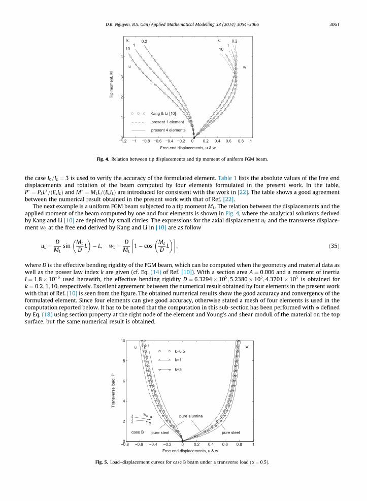
The next example is a uniform FGM beam subjected to a tip moment ML. The relation between the displacements and theapplied moment of the beam computed by one and four elements is shown in Fig. 4, where the analytical solutions derivedby Kang and Li [10] are depicted by small circles. The expressions for the axial displacement uL and the transverse displace-ment wL at the free end derived by Kang and Li in [10] are as follow

uL ¼D

MLsin

ML

DL

� �� L; wL ¼

DML

1� cosML

DL

� � ; ð35Þ

where D is the effective bending rigidity of the FGM beam, which can be computed when the geometry and material data aswell as the power law index k are given (cf. Eq. (14) of Ref. [10]). With a section area A ¼ 0:006 and a moment of inertiaI ¼ 1:8� 10�6 used herewith, the effective bending rigidity D ¼ 6:3294� 105;5:2380� 105;4:3701� 105 is obtained fork ¼ 0:2;1;10, respectively. Excellent agreement between the numerical result obtained by four elements in the present workwith that of Ref. [10] is seen from the figure. The obtained numerical results show the good accuracy and convergency of theformulated element. Since four elements can give good accuracy, otherwise stated a mesh of four elements is used in thecomputation reported below. It has to be noted that the computation in this sub-section has been performed with / definedby Eq. (18) using section property at the right node of the element and Young’s and shear moduli of the material on the topsurface, but the same numerical result is obtained.

−0.8 −0.6 −0.4 −0.2 0 0.2 0.4 0.6 0.8 10

2

4

6

8

10


Tran

sver

se lo

ad, P

pure steel pure steel

pure alumina

k=0.5

k=1

k=5

P

case B

u w

u w

Fig. 5. Load–displacement curves for case B beam under a transverse load (a ¼ 0:5).

−1.2 −0.8 −0.4 0 0.4 0.80

2

4

6

8

10


Ecce

ntric

axi

al lo

ad, P

pure alumina

pure steel pure steel

P

uw

u wk=0.5k=1

k=5

case B

Fig. 6. Load–displacement curves for case B beam under an eccentric axial force (a ¼ 0:5).

0 0.2 0.4 0.6 0.80

0.2

0.4

0.6

0.8

1+u

w

k: 5 1 0.5

case B, α=0.5

−0.1 0 0.2 0.40

0.2

0.4

0.6

0.8

1+u

wk: 0.515

case B, α=0.5

Fig. 7. Deformed configurations corresponding to P ¼ 5 for case B beam with different values of index k.


4.2. Effect of material non-homogeneity

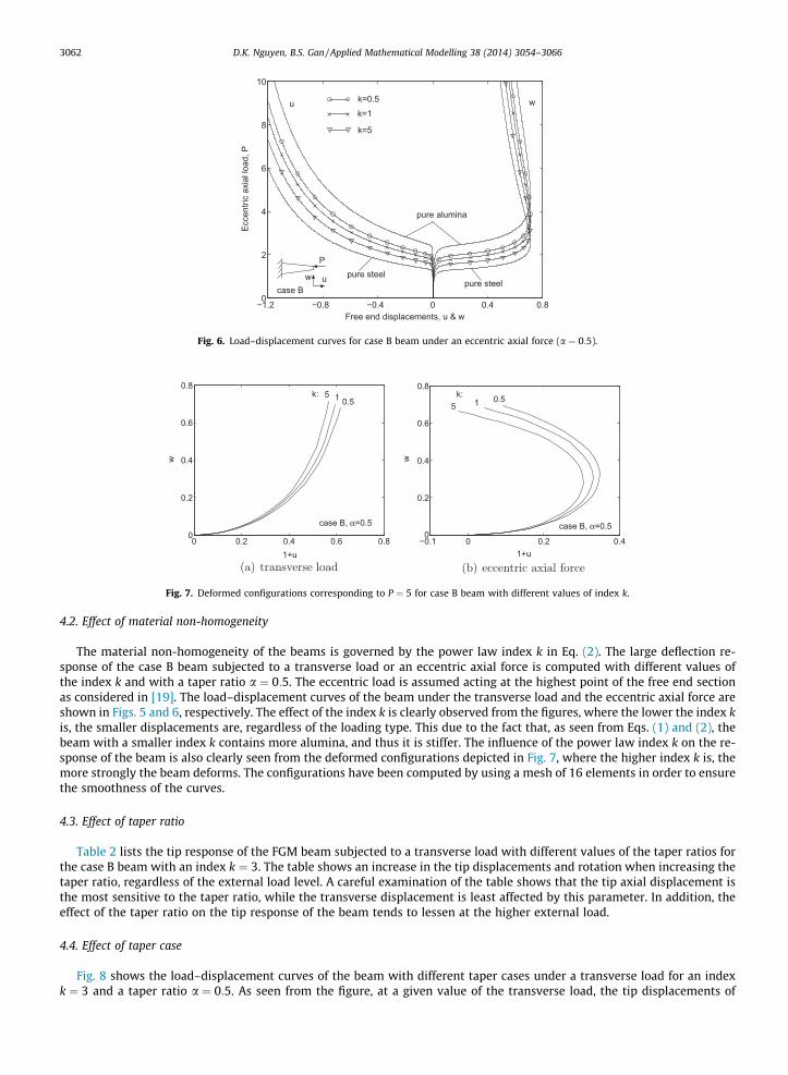
The material non-homogeneity of the beams is governed by the power law index k in Eq. (2). The large deflection re-sponse of the case B beam subjected to a transverse load or an eccentric axial force is computed with different values ofthe index k and with a taper ratio a ¼ 0:5. The eccentric load is assumed acting at the highest point of the free end sectionas considered in [19]. The load–displacement curves of the beam under the transverse load and the eccentric axial force areshown in Figs. 5 and 6, respectively. The effect of the index k is clearly observed from the figures, where the lower the index kis, the smaller displacements are, regardless of the loading type. This due to the fact that, as seen from Eqs. (1) and (2), thebeam with a smaller index k contains more alumina, and thus it is stiffer. The influence of the power law index k on the re-sponse of the beam is also clearly seen from the deformed configurations depicted in Fig. 7, where the higher index k is, themore strongly the beam deforms. The configurations have been computed by using a mesh of 16 elements in order to ensurethe smoothness of the curves.

4.3. Effect of taper ratio

Table 2 lists the tip response of the FGM beam subjected to a transverse load with different values of the taper ratios forthe case B beam with an index k ¼ 3. The table shows an increase in the tip displacements and rotation when increasing thetaper ratio, regardless of the external load level. A careful examination of the table shows that the tip axial displacement isthe most sensitive to the taper ratio, while the transverse displacement is least affected by this parameter. In addition, theeffect of the taper ratio on the tip response of the beam tends to lessen at the higher external load.

4.4. Effect of taper case

Fig. 8 shows the load–displacement curves of the beam with different taper cases under a transverse load for an indexk ¼ 3 and a taper ratio a ¼ 0:5. As seen from the figure, at a given value of the transverse load, the tip displacements of

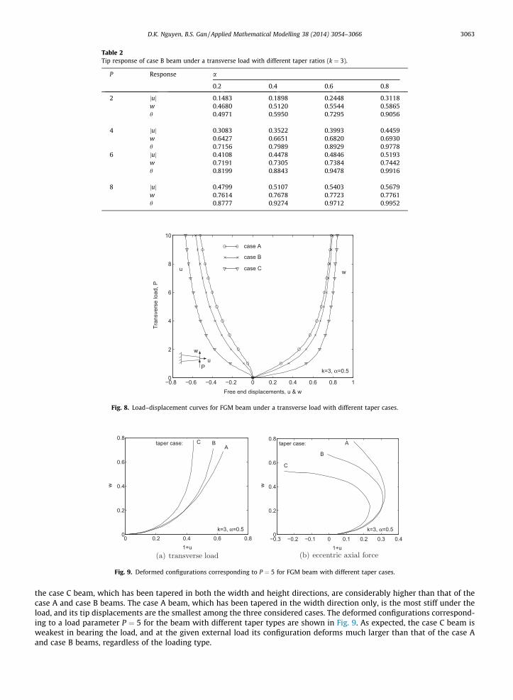
Table 2Tip response of case B beam under a transverse load with different taper ratios (k ¼ 3).

P Response a

0.2 0.4 0.6 0.8

2 juj 0.1483 0.1898 0.2448 0.3118w 0.4680 0.5120 0.5544 0.5865h 0.4971 0.5950 0.7295 0.9056

4 juj 0.3083 0.3522 0.3993 0.4459w 0.6427 0.6651 0.6820 0.6930h 0.7156 0.7989 0.8929 0.9778

6 juj 0.4108 0.4478 0.4846 0.5193w 0.7191 0.7305 0.7384 0.7442h 0.8199 0.8843 0.9478 0.9916

8 juj 0.4799 0.5107 0.5403 0.5679w 0.7614 0.7678 0.7723 0.7761h 0.8777 0.9274 0.9712 0.9952

−0.8 −0.6 −0.4 −0.2 0 0.2 0.4 0.6 0.8 10

2

4

6

8

10


Tran

sver

se lo

ad, P

case A

case B

case C

Pu

w

wu

k=3, α=0.5

Fig. 8. Load–displacement curves for FGM beam under a transverse load with different taper cases.

0 0.2 0.4 0.6 0.80

0.2

0.4

0.6

0.8

1+u

w

taper case: A

BC

k=3, α=0.5

−0.3 −0.2 −0.1 0 0.1 0.2 0.3 0.40

0.2

0.4

0.6

0.8

1+u

w

taper case: A

B

k=3, α=0.5

C

Fig. 9. Deformed configurations corresponding to P ¼ 5 for FGM beam with different taper cases.


the case C beam, which has been tapered in both the width and height directions, are considerably higher than that of thecase A and case B beams. The case A beam, which has been tapered in the width direction only, is the most stiff under theload, and its tip displacements are the smallest among the three considered cases. The deformed configurations correspond-ing to a load parameter P ¼ 5 for the beam with different taper types are shown in Fig. 9. As expected, the case C beam isweakest in bearing the load, and at the given external load its configuration deforms much larger than that of the case Aand case B beams, regardless of the loading type.

Table 3Tip response of case A beam under a transverse load with different aspect ratios (k ¼ 3;a ¼ 0:5).

P Response L=h0

50 25 20 15 10

4 juj 0.3042 0.3047 0.3050 0.3056 0.3071w 0.6393 0.6394 0.6394 0.6398 0.6417h 0.7099 0.7082 0.7073 0.7056 0.7020

8 juj 0.4766 0.4769 0.4772 0.4777 0.4791w 0.7601 0.7603 0.7607 0.7618 0.7659h 0.8737 0.8711 0.8697 0.8673 0.8618

Table 4Tip response of case C beam under a transverse load with different aspect ratios (k ¼ 3;a ¼ 0:5).

P Response L=h0

50 25 20 15 10

4 juj 0.5152 0.5154 0.5155 0.5159 0.5170w 0.7547 0.7552 0.7558 0.7574 0.7626h 0.9626 0.9592 0.9575 0.9544 0.9479

8 juj 0.6346 0.6348 0.6350 0.6355 0.6369w 0.8242 0.8259 0.8274 0.8310 0.8420h 0.9903 0.9858 0.9834 0.9795 0.9710


4.5. Effect of aspect ratio

The tip responses of the case A and case C beams with different values of the aspect ratio, L=h0, subjected to a transverseload are given in Tablse 3 and 4 for the case k ¼ 3 and a ¼ 0:5, respectively. While both the tip axial and transverse displace-ments increase when reducing the aspect ratio, the tip rotation reduces, regardless of the external load level and the tapercase. Examining the tables in more detail, one can see that while the tip axial displacement of the case A beam is more sen-sitive to the aspect ratio comparing to the case C beam, the tip transverse and rotation of the case A beam are much lesssensitive to the aspect ratio than that of the case C beam.

4.6. Beam with different materials

To study the large deflection behaviour of the FGM beam formed from different materials, in addition to the beam formedfrom steel and alumina (SA) examined above, two other cantilever FGM beams, one formed from aluminum and steel (AS),and the other from aluminum and alumina (AA) are considered in this Sub-section. The Young’s modulus and Poisson’s ratioof aluminum are 70 GPa and 0.3, respectively [31].

−0.8 −0.6 −0.4 −0.2 0 0.2 0.4 0.6 0.8 10

2

4

6

8

10


Tran

sver

se lo

ad, P

Beam material:

AS

AA

SA

w u

PCase C, k=3, α=0.5

Fig. 10. Load–displacement curves for case C beam formed from different materials under a transverse load.

0 0.1 0.2 0.3 0.4 0.50

0.2

0.4

0.6

0.8

1

1+u

AS AASA

case C, k=3, α=0.5

Beam material:

w

0 0.1 0.2 0.3 0.4 0.50

0.2

0.4

0.6

0.8

1

1+u

AS AASA

case C, k=3, α=0.5

Beam material:

w

Fig. 11. Deformed configurations for case C beam formed from different materials under a transverse load.


Fig. 10 shows the load–displacement curves for the case C beam formed from the different materials under a transverseload for the case k ¼ 3 and a ¼ 0:5. It is necessary to note that for the purpose of comparison, the load P of all the curves inthe figure is normalized by the Young’s modulus of steel according to Eq. (34). At a given value of the external load, the AAbeam with the Young’s modulus of the bottom surface material is just one third of that of the SA beam, deforms much largerthan the SA beam. The AS beam with the Young moduli of the materials on both the top and bottom surfaces are lower thanthat of the SA beam is the most flexible. The deformed configurations of the beams at two values of the load parameter,namely P ¼ 5 and P ¼ 10, as depicted in Fig. 11 also confirm the influence the materials on the large deflection behaviourof the beam.

5. Conclusions

The large deflections of tapered FGM beams subjected to the end forces have been studied by the finite element method. Anonlinear first order shear deformable beam element, using the polynomials as solutions of a uniform homogeneous Timo-shenko beam segment to interpolate the transverse displacement and rotation, has been formulated in the context of the co-rotational formulation. The large deflection response of a cantilever FGM beam with various taper cases has been computedby using the arc-length control algorithm in combination with the Newton–Raphson method. The numerical examples haveshown that the formulated element is capable to give accurate response by using just several elements. A parametric studyhas been given to examine the effect of the non-homogeneity material, the taper ratio as well as the aspect ratio on the largedeflection behaviour of the beams.

Though the numerical examples in the present work were presented for the cantilever beam, the element formulated inthe present work is independent of the boundary conditions, and thus the finite element procedure described in this papercan be employed to analyze the beams with other boundary conditions.

Acknowledgement

The financial support from Vietnam NAFOSTED to the first author is gratefully acknowledged.

Appendix A. Supplementary data

Supplementary data associated with this article can be found, in the online version, at http://dx.doi.org/10.1016/j.apm.2013.11.032.

References

[1] M. Koizumi, FGM activities in Japan, Compos. Part B Eng. 28 (1997) 1–4.[2] V. Birman, L.W. Byrd, Modeling and analysis of functionally graded materials and structures, Appl. Mech. Rev. 60 (2007) 195–216.[3] B.V. Sankar, An elasticity solution for functionally graded beams, Compos. Sci. Technol. 61 (2001) 689–696.[4] A. Chakraborty, S. Gopalakrishnan, J.R. Reddy, A new beam finite element for the analysis of functionally graded materials, Int. J. Mech. Sci. 45 (2003)

519–539.[5] A. Chakraborty, S. Gopalakrishnan, A spectrally formulated finite element for wave propagation analysis in functionally graded beams, Int. J. Solids

Struct. 40 (2003) 2421–2448.[6] R. Kadoli, K. Akhtar, N. Ganesan, Static analysis of functionally graded beams using higher order shear deformation beam theory, Appl. Math. Model. 32

(2008) 2509–2525.[7] M.A. Benatta, I. Mechab, A. Touns, E.A. Adda Bedia, Static analysis of functionally graded short beams including warping and shear deformation effects,

Comput. Mater. Sci. 44 (2008) 765–773.[8] K.V. Singh, G. Li, Buckling of functionally graded and elastically restrained nonuniform column, Compos. Part B Eng. 40 (2009) 393–403.



http://refhub.elsevier.com/S0307-904X(13)00768-3/h0005













[9] Y.A. Kang, X.F. Li, Bending of functionally graded cantilever beam with power-law nonlinearity subjected to an end force, Int. J. Non-linear Mech. 44(2009) 696–703.

[10] Y.A. Kang, X.F. Li, Large deflection of a non-linear cantilever functionally graded beam, J. Reinf. Plast. Compos. 29 (2010) 1761–1774.[11] Y.Y. Lee, X. Zhao, J.N. Reddy, Postbuckling analysis of functionally graded plates subjected to compressive and thermal loads, Comput. Methods Appl.

Mech. Eng. 199 (2010) 1645–1653.[12] Y. Huang, X.F. Lin, A new approach for free vibration of axially functionally graded beams with non-uniform cross-section, J. Sound Vib. 329 (2010)

2291–2303.[13] V. Kutiš, J. Murín, R. Belák, J. Paulech, Beam element with spatial variation of material properties for multiphysics analysis of functionally graded

materials, Comput. Struct. 89 (2011) 1192–1205.[14] A.E. Alshorbagy, M.A. Eltaher, F.F. Mahmoud, Free vibration characteristics of a functionally graded beam by finite element method, Appl. Math. Model.

35 (2011) 412–425.[15] N. Wattanasakulpong, B.G. Gangadhara, D.W. Kelly, Thermal buckling and elastic vibration of third-order shear deformable functionally graded beams,

Int. J. Mech. Sci. 53 (2011) 734–743.[16] A. Shahba, R. Attarnejad, M.T. Marvi, S. Hajila, Free vibration and stability analysis of axially functionally graded tapered Timoshenko beams with

classical and non-classical boundary conditions, Compos. Part B Eng. 42 (2011) 801–808.[17] M. Aminbaghai, J. Murín, V. Kutiš, Modal analysis of the FGM-beams with continuous transversal symmetric and longitudinal vibration of material

properties with effect of large axial force, Eng. Struct. 34 (2012) 314–329.[18] D.K. Nguyen, B.S. Gan, T.H. Le, Dynamic response of non-uniform functionally graded beams subjected to a variable speed moving load, J. Comput. Sci.

Technol. (JSME) 7 (2013) 12–27.[19] R.D. Wood, O.C. Zienkiewicz, Geometrically nonlinear finite element analysis of beams, frames, arches and axisymmetric shells, Comput. Struct. 7

(1977) 725–735.[20] W.L. Cleghorn, B. Tabarrok, Finite element formulation of a tapered Timoshenko beams for free lateral vibration analysis, J. Sound Vib. 152 (1992) 461–

470.[21] G. Baker, On the large deflections of non-prismatic cantilevers with a finite depth, Comput. Struct. 46 (1993) 365–370.[22] B.K. Lee, J.F. Wilson, S.J. Oh, Elastica of cantilevered beams with variable cross section, Int. J. Non-linear Mech. 28 (1993) 579–589.[23] M. Brojan, T. Videnic, F. Kosel, Large deflections of nonlinearly elastic non-prismatic cantilever beams made from materials obeying the generalized

Ludwick law, Meccanica 44 (2009) 733–739.[24] R. Attarnejad, S.J. Semnani, A. Shahba, Basic displacement functions for free vibration analysis of non-prismatic Timoshenko beams, Finite Elem. Anal.

Des. 46 (2010) 916–929.[25] A. Shahba, R. Attarnejad, S.J. Semnani, V. Shahriari, A.A. Dormohamamadi, Derivation of an efficient element for free vibration analysis of rotating

tapered Timoshenko beams using basic displacement functions, Proc. IMechE Part G J. Aerosp. Eng. 226 (2012) 1455–1469.[26] M.A. Crisfield, Non-linear Finite Element Analysis of Solids and Structures, Volume 1: Essentials, John Wiley & Sons, Chichester, 1991.[27] C. Pacoste, A. Eriksson, Beam elements in instability problems, Comput. Methods Appl. Mech. Eng. 44 (1997) 163–197.[28] D.K. Nguyen, A Timoshenko beam element for large displacement analysis of planar beams and frames, Int. J. Struct. Stab. Dyn. 12 (2012), http://

dx.doi.org/10.1142/S0219455412500484.[29] J.B. Kosmatka, An improve two-node finite element for stability and natural frequencies of axial-loaded Timoshenko beams, Comput. Struct. 57 (1995)

141–149.[30] J.R. Reddy, On locking-free shear deformable beam finite elements, Comput. Methods Appl. Mech. Eng. 149 (1997) 113–132.[31] G.N. Praveen, J.N. Reddy, Nonlinear transient thermoelastic analysis of functionally graded ceramic-metal plates, Int. J. Solids Struct. 35 (1998) 4457–

4476.



































http://dx.doi.org/10.1142/S0219455412500484

http://dx.doi.org/10.1142/S0219455412500484






1-s2.0-s0307904x13007683-main

Documents