ELSEVIER Journal of Wind Engineering

and Industrial Aerodynamics 58 (1995) 277-292

,~URN~. OF

Reformulation of the momentum theory applied to wind turbines

Rica rdo A. P r a d o

Departamento de Mecimica Aplicada, Facultad de lngenieria, Universidad Nacional del Comahue, calle Buenos Aires No. 1400, 8300 Neuqudn, Argentina

Received 2 January 1994; accepted 21 June 1995

Abstract

The aim of the present paper is to propose modifications to the Dyment formulation of the momentum theory applied to wind turbines. Although the hypotheses established by Dyment in order to modify the classical Betz wind turbine theory are considered valid, an alternative model is proposed to represent the streamtube that flows through the actuator disc and defines the turbine wake contour. In the present model a source is added to include the effects of a divergent streamtube, whose geometry is defined by the intensity of the source and its position with respect to the disc that simulates the horizontal-axis wind turbine. As an example, for a given position of the rotor disc relative to the source, the characteristic coefficients of the turbine and the geometry of the bounding streamtube, are obtained for the maximum output power condition. These results are compared with those obtained from the Betz and Dyment models.

1. Introduction

The momentum theory applied to propellers (called Rankine-Froude theory) assumes that the propeller can be represented by means of a fiat and infinitely thin actuator disc of radius R that supports an uniform pressure difference on its surface. Other assumptions related to this theory are: The disc is immersed in a well-defined coaxial streamtube z. Inside that streamtube, the flow is con- sidered practically one-dimensional. The fluid is incompressible. The flow rotation imposed by the propeller is not considered. The static pressure, infinitely far ahead and behind the actuator disc is constant and equal to the freestream static pressure,

Poo. As stated by Theodorsen [1], although an actuator disc cannot be considered as

a mathematical limit for the description of a propeller, the momentum theory gives

0167-6105/95/$09.50 © 1995 Elsevier Science B.V. All rights reserved SSDI 0167-6105(95)00021-6

278 R.A. Prado/J. Wind Eng. Ind. Aerodyn. 58 (1995) 277-292

q

- i

i

-!

-i

P,

V

p - p

.. v ,! 4

%

q

3 ! .4

j 7.,,(I b)

i V (~-20) . -1

4 I [ -4

~ 0

Fig. 1. Flow model according to the Betz theory.

:z + , ,

×

a simplified representation which enables the general properties of the system to be obtained.

Betz applied the theory to the case of a horizontal-axis wind turbine [2]. Since the turbine extracts kinetic energy from the wind, the streamtube that traverses the disc has to become wider as it flows downstream (Fig. 1).

At infinity ahead of the disc, the velocity field is given by the freestream velocity, V~, and the pressure field by the freestream static pressure, p~.

At the disc, the velocity has decreased by a fraction a with respect to V~,, and the pressure distribution shows a discontinuity. The velocity crossing the disc, Vd = V~ (1 -- a), is assumed constant. The disc supports a uniform pressure difference, Ap = p' - p", where p' > p~ and p" < p~. This pressure difference generates, on the area S = rcR 2 of the disc, a thrust T = A p S .

At infinity behind the disc, the pressure recovers the value of the freestream static pressure, p~. The flow outside the streamtube that crosses the actuator disc shows a velocity equal to V~, but the air flowing inside the streamtube has a velocity equal to V~ (1 - b), b being greater than a.

By analogy with Rankine-Froude theory, Betz assumed that the air inside the streamtube r flows without pressure losses. Therefore, it is possible to apply the Bernoulli equation between far upstream and just ahead of the disc, and between just behind the disc and far downstream, changing the Bernoulli constant when the flow crosses the disc.

R.A. Prado/J. Wind Eng. Ind. Aerodyn. 58 (1995) 277-292 279

P~

W

P~ p'

~ ~ P~ P~ V~ V~

P = P~ O-b)

V ( I -o) ( l -a )

L

X : - c ~ X : 0 X : + '>:

Fig. 2. Flow model according to the Dyment theory (see Ref. [3], Fig. 2).

X

Dyment [3] presented a modification to the Betz theory considering that, since the flow inside the streamtube z is continuously retarded, the internal streamtube edges are represented by shear layers that develop eddies. These eddies imply losses, and consequently, the Bernoulli equation cannot be applied inside the streamtube z. Therefore, in the Dyment model, the Bernoulli equation is applied only to the air flowing outside the streamtube r.

As a result of the Dyment model (Fig. 2), due to the pressure field downstream of the disc being given by p~, the retarded air flows with no losses inside the streamtube portion behind the disc. However, since a shear layer is still present, there is a contra- diction between hypotheses and results.

Theodorsen [1] considered that in the application of momentum theory to propel- lers, the external flow (i.e. the flow that surrounds the streamtube z) may be analysed as the superposition of a sink "at the origin" to the freestream field. This superposition is valid since the sink does not disturb the flow conditions at infinity.

Following the Theodorsen assertion, when applying the momentum theory to wind turbines, the potential external flow could be represented by the superposition on the freestream field of a source whose strength and position with respect to the actuator disc should be determined.

In accordance with the Dyment procedures, the Bernoulli equation is applied only to that external flow. Also, since the swirl introduced by the rotor is generally small [4], it is neglected in the present model.

280 R.A. Prado/d. Wind Eng. Ind. Aerodyn. 58 (1995) 277-292

2. Procedure

According to potential theory, the axisymmetric flow determined by the superposi- tion of a uniform stream with velocity V~ and a source of strength k placed at the origin of the coordinates is determined for the whole field (r, 0) by the streamfunction

~(r, O) = - ~ V.~ r- sin- 0 + k cos O. (1)

This superposition defines the flow field called m o d e l A .

For a source strength given by k = V,~ 6 2, a body of revolution is defined by the streamfunction 7~(r, O) = V~ 6 2 (the so-called Rankine axisymmetric body), where 6 represents the distance between the source and the body vertex. The body contour is determined by

6 r(O) -- . (2)

sm (0/2)

By transforming to Cartesian coordinates Eq. ~2) is rewritten as

//1 A.¢.2 X 2 3,= _ + ~ ( ~ , - + x v / x 2 + 8 6 2 ) . x~> - 6 . (3t

The presence of the blunt body generates a particular streamtube r that, in coincid- ence with the disc abscissa x = Xo, has a radius equal to the radius of the disc, R. The disc position (x = x0) does not necessarily coincide with the source position (x = 0).

Having defined the geometry of the streamtube r, the Rankine axisymmetric body is eliminated, and following the Betz and Diment models, a one-dimensional axial flow is considered in the interior of the streamtube r. In this configuration (called m o d e l B), the external flow is the same to that defined by model A (i.e. source plus freestream). Fig. 3 shows models A and B.

3. Velocity field

For the external flow in model B, and for every point of the field in model A, the streamfunction is

~(r, 0) = V~ (6 2 cos 0 --½r e sin e 0)

and the velocity components are

- V~,o [cos 0 + ( 6 / r ) 2 ] , v , - r 2sin0c~0

In the Cartesian coordinate system (x, y)

Vx = Vo sin 0 - v, cos O,

(4)

1 &0 - V~ sinO. (5)

~ ' o - r s i n O ?r

G, = - Vo cos 0 + tJ, sin O, (6)

R.A. Prado/J. Wind Eng. Ind. Aerodyn. 58 (1995) 277-292 281

X ~ - c o

~y

p~ I

v~ I

"F

P® i , 72(

voo

"1-

I b......-J

I

I

I

x : 0

g~o-o)

p ' l ~ R

p~

V~

26

"7

Fig. 3. Models A and B for the representation of the streamtube internal flow. The external flow is the same in both models.

then

( vx(x,y) = V~ 1 ~ (X 2 + y2)a/2,],

The modulus of the velocity vector is

2 V(x, y) = I V(x, Y) I = x / ~ z + vr,

therefore, from Eqs. (7),

= VZ~(1 + VZ(x, y) \

2XO 2 64 ) (X2 .~_ y2)3/2 + (X 2 _~_ y2)2 "

y62 ) vy(x, y) = V~ (x 2 + y2)3/2 '

In particular, the velocity distribution along the y axis (x = O) is given by

vx(O, y) = V~o, v,(o, y) = v~ ~ , v2(o, y) = v ~ l +

(7)

(8)

(9)

282 R.A. Prado/Y. Wind Eng. Ind. Aerodyn. 58 (1995) 277 292

4. Equivalence relationship between models A and B

The volumetr ic flow rate, q (being measured in model A through the annular section defined at the abscissa Xo, between the Rankine axisymmetr ic body (Eq. (3)) and the s t reamtube r), is given by

2r~ R R

q = c.dXo, y)ydyd~p = 27rI~, I -} Ix 2 + v2)3/2 ydy ,

0 FZq. 13 ) [{q, (.'.)

q = 7rV_~R 2 1 -- 3~-2 (4~52 - -'G + .x'~x'xg + 862)

,5-' " - (10) + 2 ~ Xo , 2 r 2 ~ ' x/462 + .'q~ + xo \ - o + 8( ~2 ~ /R + Xo

Since the s t reamtube r has the same contigurat ion in both models A and B, the volumetric flow rate given by Eq. (10) should be the same as the volumetric flow rate that flows through the ac tua tor disc in model B. Therefore,

q = r r V , R2(1 a). ( l l )

Equat ing Eqs. {10) and (11), gives

a = ~ ( 4 ¢ ~ 2 -- .% + x o \ ' . ' q { + 8~21

- 2 R~ Xo ," . 2 .v/R 2 ~//462 + x~ + Xo \. .xo + 832 + x

and by introducing the nondimensional variables

(~ = R / & c = Xo/6

the following equat ion is obtained.

a = ~ ( 4 - . + r x & 2 + 8 ) :-,c~ ] - ~ ",\ 4 + c 2 +~:w'c /~+8 V/- ~ 2 + e 2

Letting

= 4 - ~:2 + c\/.c2 + 8,

vS . l] = i/-- ,~;2 I X v 4 + + ~: \,,. c + 8

(12)

R.A. Prado/J. Wind Eng. Ind. Aerodyn. 58 (1995) 277-292 283

the following expression, for ~ as a function of a and e, results

¢6(¼aZ ) + ~ 4 [ a ( f l _ ¼~ + ¼ae2)] + ¢2[fl2 + ~ u z _ ½eft + aeZ(fl-¼a)] + ez( flz + ~6az -½eft - I) = 0. (13)

Since the following relations are true,

fl -¼~ = - I, flz + ~6~2 -½eft = i

Eq. (13) is simplified to

~4 + ~2 ( e 2 - ! ) + a4--g(1- ae2) = 0,

which has the solution

~z = 1 [(4 - ae') + ew/-~ + ae2)]. (14)

Eq. (14) establishes the equivalence between models A and B since it relates the variables R, 6, Xo and a, having the values of a and Xo/6 as the input variables. However, since it is better to have a and xo/R as the input variables, the new variable e = xo/R (i.e. e = e0 is introduced and for e 7> 0, it follows that

~2=_2 1 + . (15) a

5. Determination of the coefficient b

Since at x = + oo the Rankine axisymmetric body has a radius 26, at x = + oo the streamtube z will have a radius R +~, and from the continuity condition in model A, the volumetric flow rate q is

q = V~on [RZ+~ - (26)1]. (16)

This must equal that flowing inside the bounding streamtube in model B, given by Eq. (11), so that

R2+oo = 462 + R2(1 - a)

and therefore

R+o~ 1 R =-~ x/(1 -- a)~2 + 4. (17)

Applying the continuity condition to the streamtube z in model B, it follows that

V~rrR2~ = V~(1 - a)ltR 2 = Vow(1 - b)nR2+~

284 R.A, Prado/J. Wind Eng, Ind. derodyn. 58 H995)27~292

and therefore, 2 R+~(1 - b) = R 2 ( 1 - a). (18)

Equating Eqs. (17) and (18), one obtains the relationship between the reduction of velocity at the disc, a, and the reduction of velocity at infinity downstream, b, for a given value of e,

4 b - (19)

(1 - - a ) ~ z + 4'

where ~2 is given by (15).

6. Geometry of the streamtube z

The streamfunction that defines the streamtube r is 1 2 • 2 ~o = V-~(~2cosOo--~rosln 0o),

where

2 R 2, xo _ Xo R R r 2 = x o + c o s 0 o - s i n 0 o - - ro o x / ~ - ~ ' ro xf~o2 + R 2

Therefore,

( a2x 0 1 2 R2 ( e ~ ) . (20) 2

In order to determine the Cartesian coordinates (x, y) of that streamfunction, one sets

1 ( 2~2x ~ 7'(x, y) = - ~ v . y2 --- ~ ] ~o- (21)

Defining

2e 2 = 1 , Y, = x / R , y = y / R

~2 ~-~ + 1

and equating Eqs. (20) and (21), it follows that

22 ~2 _ _ - - ~ g 2 f ~ + y2

having the following polynomial form,

y6 + 374(22 -- 22) + 372(22 _2222) + 22(22 _ 4/(4) = 0. (22)

The geometry 37 = 37 ( - ~ < £ < + 0o) of the streamtube z is determined by solving Eq. (22) when the values of a and e are given. Particularly, at the origin, the streamtube

radius is y(0) = x/2R.

. ~ / > ~f > ~ /y jx pue Ox ~ x ~ 0 aoj 'z oqnltueoals oql jo op!s leUaOlxo oql (!.t!)

,(Ox = x ' ~ / ~ ~f ~ 0) os!p ao len loe oql (!!) '.(0 = x 'oo > 4" > ~ /~ jx ) ,VV uo!loos ae lnuue oql (9

:,{q

UOA~ Oa~ SU!~tuop Oral oql JO so .uepunoq uotutuoo oq.l "os!p ~ol~nlo~ oql jo tu~o~ls - u ~ o p pooeld II u!e tuop oql pue 'os!p ao len loe oql jo tueoalsdn pooeld I u!e tuop oql :9 pug ~ "s$!~l u~ uA~oqs s! 1! Se pougop oae su!etuop o ~ 'fl Iopotu uI

sasso ! aanssaJd aql jo uo.~leu.nuaala(I "L

"90L6"0 = y__//x 'osgo lgql uI "L6E'0 = n pue 0gE'0 = a aoj ~poq oulotutu,(s!xg OUplUe~I oql pug z oqnlturoals oql smoqs 17 "~!A

"(ou!l

pmlop-qsep) ,~poq o!Jlatutu,(s!xr OUplU~I ~u!puodso~1oo oql p u t u!~!~o oql 1~ oo.mos oql '(OU!l poqs~p) os!p aol~nlo~ Otll s! u ~ o q s o s l v "(ou!I p!los)0gE'0 = a pue L6U0 = v ~oj z oqnltu~o~ls *ql jo uot . l~n~tjuo D "'e "~!A

g £'L c3"0 0 g 'O- t.- ~'1,- Z - - - ' I" I ' ' ~ -

. . . . . . . . . . ~ - . . . . . . . . . -, ; . . . . . . t

. . . . . . . . . . . . . . . . . . . . . . . . . i . . . . . . . . . . . . . ~ . . . . . . ,~ . . . . . . . . . . . . . . . . . ~ . . . . . . . . . . . . . . . . . . . . . . . . . . . . . . . . . . . . . . . . . . . : : : x : :

: : i L

; i t ! ; : ? 1 ,' [

i / : : i : / :

1

i i i

c j o ~ o = q L 6 E O = o

~ ' 0 -

0

. . . . . ~ . . . . . . . . . . . . ~ . . . . . . . . . . g ' O

i ,

~ :

. . . . . . . . . . . . . . . . . . . . . . . . . . . ~ . . . . . . . . . . . . . . . . ~ ' L

OgZO = a

; ; r 3

~SE ~6g-LLg (~66I) gg "u'fp°aav "pul "Su~t pu!M "F/opvad "V'~t

286 R.A. Prado/J. Wind Eng. Ind. Aeroclvn. 58 (1995) 277-292

V --V=

X -- ~

V --V®

y = + c,~ V = v , = V ~

V~ zV=

y = - . V v ~ ,

p(o,y)-p~

i

I , R

L 1 X i

0

k

x ; O

B' A ~

p, _ p~.,

V = V~oO-o)

Fig. 5. Schematic representation of the control volume for the domain 1 showing the axial velocity and the relative pressure distributions over its contour. The pressure is relative to the freestream static pressure, p~. This domain includes the anterior portion of the streamtube r and the external flow for x~<0.

Applying the Bernoulli equation to the external flow, the pressure distribution on section AA' can be determined. Then,

p(O,y) p~ =~pL ~ - V 2 ( 0 , y ) ] = ½ p ,~ y ,

where p denotes the air density.

R.A. Prado/J. Wind Eng. Ind. Aerodyn, 58 (1995) 277-292 287

V = V®

p(0,y)- p.

A ~

p"_ p®

o

V~(I-c

p(~,y)- p°

A'

y _--+oo V = v ~ : V .

V x = V~

p(O,y)- p®

X = X o

y :+oo V : v, :V~

v=v.

X = -I.~o

V.O-b)

- - C

V=V®

C'

Fig. 6. Same as in Fig. 5 for domain I1. This domain includes the posterior portion of the streamtube z and the external flow for x > 0. As in domain I, the portion AA" of the control volume is represented by the external side of the streamtube z; therefore, there is no flow through that surface.

In order to apply the momentum conservation theorem in the axial direction, the axial pressure force on the section AA', F1, must be determined as follows

2 ~ oo

F1 = f Rf~[P(0'Y)-p~]ydyd(p =

~ p V Z R 2

22~ 4 (23)

288 R.A. Prado/J. Wind Eng. Ind. Aerodyn. 58 (1995) 277 292

,~ R i

i J i

i i

X

Fig. 7. Conical app rox ima t ion to the shape of the s t r eamtube ~ for 0 < x ~< \,~.

On the left-hand side of the ac tuator disc, the axial force acting, t:2, is

F 2 = (p' - p ~ . ) S =- (p ' p~ ) g R 2. (24)

On the r ight-hand side of the ac tuator disc, the axial force acting, F3, is

1:3 = (p" - p ~ ) S = (p" - p ~ ) ~ R 2. (25)

The axial force, -~4, acting on the streamtube section 0 ~< x ~< x0, can be computed assuming that the segment AA" can be rectified (as in Fig. 7), so that

tan7 R(1 ' - = - ' - = - x / 2 ) / X o (1 v")o)/e -~ (y R x / 2 ) / x

and

o Rx,~

(26)

R.A. Prado/J. Wind Eng. Ind. Aerodyn. 58 (1995) 277-292 289

therefore, in nondimensional variables,

F, 1

2 -- 233V/2 + tan_2 30] 3/2 tan7 tan2y + ~72(1

+ y¢-4 ) t-an--~ + 372(1 + tan-2~)

In the domain I, from the axial momentum equilibrium, it follows that

--(p ' - p o ~ ) n R 2 = F, - Fa + pV~o(l - a ) r t R 2 [ V ~ ( l - a) - V~o].

In the domain II, from the axial momentum equilibrium, it follows that

(p" -p~)nR z = - F 1 + F4 + pVo~(1 - a ) r t R 2 [ V ~ ( l - b) -V~(1 - a)].

The pressure losses inside the streamtube z corresponding to the anterior and posterior portions are determined by comparing the total pressures. Also, let F be defined by F = F1 - F4.

For the anterior portion of the streamtube z, the losses are given by

1 2 1 2 ~' = (po~ + ~ p V ~ ) - [ p ' + ~pV~(1 - a ) 2 ]

~' = pv~[-~a"2 "t 2 + F / p V 2 x R 2) (27)

and for the posterior portion of the streamtube r, the losses are given by

1 2 1 2 ~" = [p" + xpVo~( l - a) 2] - [Po~ + - ~ p V . ( 1 - b)2],

~" = pV2~{(1 - a)(a - b) + ½[(l - a) 2 - ( l - b) 2] - F / p V ~ T z R 2 } ,

~tl 2 1 = pVoo [ - ~ ( a - b) 2 - e / p V ~ r t R 2 ] . (28)

The expressions for ~' and ~" must both be positive for any pair of values (a, e), for consistency of the model.

8. Characteristic coefficients of the wind turbine - Example

For a wind turbine, the thrust and output power coefficients are defined as follows: Thrust coefficient,

2T 2Ap c T = = = 2 ( 1 - a ) b ,

since Ap = p' -p" = p V ~ [a(1 - a) - (1 - a)(a - b)] = p V 2 (l - a)b.

2 9 0 R.A. Prado/'J. Wind Eng. Ind. Aerodyn. 58 (1995) 277-292

1

0 9 -

0 . 8 -

3 7 -

0 6 -

3.5

0 .~ , -

9 . 3 -

Betz'modeF L)yment's model present model (e = 0.25)

L

) 5 \ , 4\, ,

3.1

0 0.1 0.2 0,3 0,4 05 0.6 0.7 0.8 0.9

Fig. 8. Thrust coefficient, C~, versus the coefficient of velocity reduction at the disc, a , according to the Betz and Dyment theories and the present model for e - 0 . 2 5 . For the latter one, the solid line corresponds to the cases where the pressure loss coefficients for the posterior portion of the streamtube r , ~"/pV~, are positive.

Output power coefficient,

2 P o 2 T V ~ (1 a)

CPa [)V3,S p V 3 , S = C-r41 -- a ) = 2{1 - a)2b.

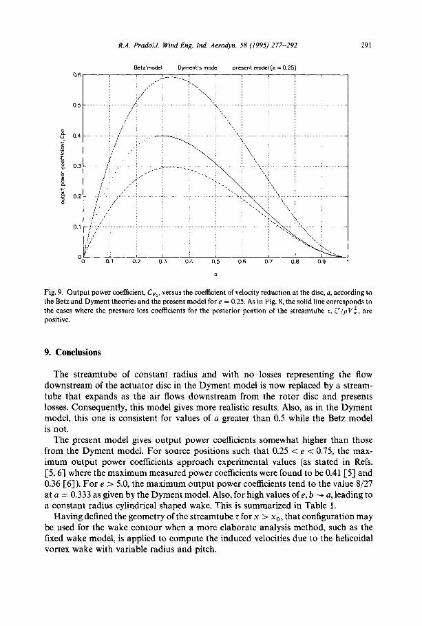
From the Betz theory, b = 2a. On the other hand, the Dyment model gives b = a. In both models, the maximum output power condition is reached when a = 0.333, being Ceo(max) = 0.5296 (Betz) and Ces(max) = 0.2963 (Dyment).

The present model reaches a maximum output power condition depending on the pair of values (a, e), providing if' and (" are positive. For example, when e = 0.250 the maximum is reached for a = 0.297. Under that condition it follows that b = 0.405, (' = 0.0378, ~'" = 0.0005, Cr = 0.5691 and Ce,. = 0.4001. Fig. 4 shows the correspond- ing geometry of the streamtube r, as well as the source and disc positions. For that location of the disc, if" becomes negative if a < 0.277.

Figs. 8 and 9 compare, respectively, the thrust and output power coefficient distributions when e = 0.250 with those corresponding to the Betz and Dyment theories. It should be recalled that the Betz model is inconsistent for a > 0.5, since 0.5 < a < 1 produces values of b > 1.

R.A. Prado/J. Wind Eng. Ind. Aerodyn. 58 (1995) 277-292 291

0 . 6

0 . 5

o 0.4

~ 0 . 3

&

~ 0 . 2 o

0.1

0 0 0.1

8etz'model Dyment's model present model (e = 0.25)

i /

: / i \~

. . . . . . / I • i . . . . . . . . . :: . . . . . . . . . . . . . . . . . . . : . . . . . . . . . . . . . . ! . . . . . . . . . . . . . . . . . ? : , , , . . . . . . . . . . . . . . . . . . . . . . . . ,

i i / t i i i i ~ i ix i i

/ / " . i \ i

f / ~ i 4 \

0.2 0.3 0.4 0.5 0.6 0.7 0.8 0.9

Fig. 9. Output power coefficient, Ceo, versus the coefficient of velocity reduction at the disc, a, according to the Betz and Dyment theories and the present model for e = 0.25. As in Fig. 8, the solid line corresponds to the cases where the pressure loss coefficients for the posterior portion of the streamtube z, ~"/pV~,, are positive.

9. Conclusions

The streamtube of constant radius and with no losses representing the flow downstream of the actuator disc in the Dyment model is now replaced by a stream- tube that expands as the air flows downstream from the rotor disc and presents losses. Consequently, this model gives more realistic results. Also, as in the Dyment model, this one is consistent for values of a greater than 0.5 while the Betz model is not.

The present model gives output power coefficients somewhat higher than those from the Dyment model. For source positions such that 0.25 < e < 0.75, the max- imum output power coefficients approach experimental values (as stated in Refs. [5, 6] where the maximum measured power coefficients were found to be 0.41 1-5] and 0.36 1-6]). For e > 5.0, the maximum output power coefficients tend to the value 8/27 at a = 0.333 as given by the Dyment model. Also, for high values of e, b --* a, leading to a constant radius cylindrical shaped wake. This is summarized in Table 1.

Having defined the geometry of the streamtube z for x > x0, that configuration may be used for the wake contour when a more elaborate analysis method, such as the fixed wake model, is applied to compute the induced velocities due to the helicoidal vortex wake with variable radius and pitch.

292 R.A. Prado/J. Wind Eng. Ind. Aerodyn. 58 (1995) 277-292

Table 1 Comparative table for the values of the maximum output power coefficients, Ceo, and the following coefficients for maximum Ce o condition: velocity reduction at the disc, a, velocity reduction at x = + ~ , b, and pressure losses for the anterior and posterior portions of the streamtube r, ('/p V 2 and ("/p V ~, as given by the Betz and Dyment theories and the present model. For the present model, these results are showed for different nondimensional locations of the actuator disc with respect to the source position, e = xo/R

Model Betz Dyment Present

e 0.25 0.50 0.75 1.0 3.0 5.0 10.0 15.0 25.0 Cpo(max) 0.5926 0.2963 0.4001 0.3647 0.3425 0,3287 0.3015 0.2982 0.2968 0.2965 0.2964 a 0.333 0.333 0.297 0.309 0.317 0,32 0.331 0.332 0.333 0.333 0.333 b 0.667 0.333 0.405 0.382 0.367 0.357 0.337 0.334 0.334 0,333 0.333 ~'/pV~, 0 0.0556 0.0378 0.0442 0.0485 0.0511 0.0540 0.0534 0.0527 0,0522 0.0519 ( " /pV] 0 0 0.0005 0.0008 0.0004 0.0001 0.0007 0.0017 0.0028 0.0032 0.0036

Although this model is not valid for every pair of values (a, e), with appropriate values of a and e, the streamtube shape obtained by the superposition of a source and a freestream could be a reasonable approach when modelling techniques are used to represent, at least, the near wake. On the other hand, the growth rate and downwind decay of the wake are found (as stated in Refs. [7,8]) to strongly depend on the ambient turbulence level, among other variables. Therefore, the actual shape of the far wake could not be adequately represented by any of these models.

Acknowledgement

The author is very grateful to lng. A. Marchegiani who plotted Figs. 1-3 and 5-7 of the present work.

References

[1] Th. Theodorsen, Theory of propellers (McGraw-HilL New York, 1948). [2] D. Le Gouri/~res, Energie 6olienne, 2nd Ed. (Eyrolles, Paris, 1982). [3] A. Dyment, A modified form of the Betz' wind turbine theory including losses, J. Fluids Eng. 111 (1989)

356 358. [4] J.F. Ainslie, Calculating the flowfield in the wake of wind turbines, J. Wind. Eng. Ind. Aerodyn. 27

(1988) 213 214. [5] R.C. Maydew and P.C. Klimas, Aerodynamic performance of vertical and horizontal axis wind

turbines, J. Energy 5, No. 3 (1981) 189-190. [6] J.L. Tangler, Comparison of wind turbine performance prediction and measurement, J. Solar Energy

Eng. 104 (1982) 84- 88. [7] F.C. Kaminsky, R.H. Kirchhoff and L,J. Sheu, Optimal spacing of wind turbines in a wind energy

power plant, Solar Energy 39, No. 6 (1987) 467 471. [8] R.W. Baker and S.N. Walker, Wake measurements behind a large horizontal axis wind turbine

generator, Solar Energy 33, No. I (1984) 5-12.