1

Running head: 1

Polar bears of the southern Beaufort Sea 2

3

Title: 4

Polar bear population dynamics in the southern Beaufort Sea during a period of sea ice decline 5

6

Jeffrey F. Bromaghin1,8, Trent L. McDonald2, Ian Stirling3,4, Andrew E. Derocher4, Evan S. 7

Richardson3, Eric V. Regehr5, David C. Douglas6, George M. Durner1, Todd Atwood1, Steven C. 8

Amstrup1,7 9

10

1 U.S. Geological Survey, Alaska Science Center, 4210 University Drive, Anchorage, Alaska, 11

99508 U.S.A. 12

2 Western Ecosystems Technology, Inc., 2003 Central Ave., Cheyenne, Wyoming 82070 U.S.A. 13

3 Environment Canada, Science and Technology Branch, Wildlife Research Division, c/o 14

Department of Biological Sciences, University of Alberta, Edmonton, Alberta, Canada, T6G 2E9 15

4 University of Alberta, Department of Biological Sciences, Edmonton, Alberta, Canada, T6G 16

2E9 17

5 U.S. Fish and Wildlife Service, Marine Mammals Management, 1011 East Tudor Road, 18

Anchorage, Alaska 99503 U.S.A. 19

6 U.S. Geological Survey, Alaska Science Center, 250 Egan Drive, Juneau, Alaska 99801 U.S.A. 20

7 Present address: Polar Bears International, P. O. Box 3008, Bozeman, MT 59772-3008 U.S.A. 21

8 Corresponding author: jbromaghin@usgs.gov, 907-786-7086 22

23

2

Abstract 24

In the southern Beaufort Sea of the U.S. and Canada, prior investigations have linked 25

declines in summer sea ice to reduced physical condition, growth, and survival of polar bears. 26

Combined with projections of population decline due to continued climate warming and the 27

ensuing loss of sea ice habitat, those findings contributed to the 2008 decision to list the species 28

as threatened under the U.S. Endangered Species Act. Here, we used mark-recapture models to 29

investigate the population dynamics of polar bears in the southern Beaufort Sea from 2001 to 30

2010, years during which the spatial and temporal extent of summer sea ice generally declined. 31

Low survival from 2004 through 2006 led to a 25-50% decline in abundance. We hypothesize 32

that low survival during this period resulted from 1) unfavorable ice conditions that limited 33

access to prey during multiple seasons; and possibly 2) low prey abundance. For reasons that are 34

not clear, survival of adults and cubs began to improve in 2007 and abundance was 35

comparatively stable from 2008 to 2010 with approximately 900 bears in 2010 (90% C.I. 606-36

1,212). However, survival of subadult bears declined throughout the entire period. Reduced 37

spatial and temporal availability of sea ice is expected to increasingly force population dynamics 38

of polar bears as the climate continues to warm. However, in the short term, our findings suggest 39

that factors other than sea ice can influence survival. A refined understanding of the ecological 40

mechanisms underlying polar bear population dynamics is necessary to improve projections of 41

their future status and facilitate development of management strategies. 42

43

Keywords: Ursus maritimus, Arctic, climate warming, sea ice, mark-recapture, abundance, 44

survival, Cormack-Jolly-Seber, Horvitz-Thompson, demographic modeling 45

46

3

INTRODUCTION 47

The polar bear (Ursus maritimus) is a universally recognized symbol of the Arctic. Polar 48

bears prefer sea ice concentrations exceeding 50% in the shallow, productive waters over the 49

continental shelf (Durner et al. 2009, Sakshaug 2004), where ice provides a platform from which 50

polar bears can efficiently hunt marine mammals. Their primary prey are ringed (Pusa hispida) 51

and bearded (Erignathus barbatus) seals, although diet varies regionally with prey availability 52

(Thiemann et al. 2008, Cherry et al. 2011). 53

Polar bears are vulnerable to the loss of sea ice, which is projected to induce substantial 54

declines in abundance by mid-century (Amstrup et al. 2008, Hunter et al. 2010) unless global 55

greenhouse gas levels are reduced (Amstrup et al. 2010). Global temperatures will rise as 56

atmospheric greenhouse gas concentrations increase (Pierrehumbert 2011), and the Arctic has 57

warmed at twice the global rate (IPCC 2007), in part due to positive feedback mechanisms 58

referred to as Arctic Amplification (Serreze and Francis 2006, Perovich and Polashenski 2012). 59

Since the advent of satellite observations in 1979, the spatial extent of Arctic sea ice during the 60

autumn ice minimum declined by over 12% per decade through 2010 (Stroeve et al. 2012), a rate 61

of loss greater than predicted by climate models (Stroeve et al. 2007, Overland and Wang 2013). 62

Coastal areas are experiencing longer ice-free periods (Markus et al. 2009) and the remaining ice 63

is increasingly composed of thin, first-year ice (Maslanik et al. 2007, 2011) with greater potential 64

for rapid melt in subsequent years (Stroeve et al. 2012). Projections of global warming and sea 65

ice loss led to the species being listed as threatened under the U.S. Endangered Species Act in 66

2008, increasing global awareness of its status and elevating the importance of monitoring by 67

circumpolar nations (Vongraven et al. 2012). 68

4

Amstrup et al. (2008) introduced a classification of polar bear habitat into ecoregions based 69

on broad seasonal patterns of sea ice dynamics that is useful for understanding regional 70

differences in polar bear ecology (Fig. 1). However, populations sharing an ecoregion may 71

experience localized combinations of environmental and ecological conditions that elicit 72

different responses. For example, in the Seasonal Ice Ecoregion (Fig. 1), where sea ice melts 73

completely in summer and forces all bears ashore until ice re-forms in autumn, reduced access to 74

prey during prolonged ice-free periods is negatively affecting the status of some populations 75

(Stirling et al. 1999, Regehr et al. 2007, Rode et al. 2012), while high prey abundance may be 76

forestalling declines in other populations (Peacock et al. 2013). In the Divergent Ice Ecoregion 77

(Fig. 1), polar bears still have access to some ice all year, although its availability over the 78

continental shelf during summer and autumn is increasingly limited (Markus et al. 2009). 79

Despite extensive sea ice loss throughout the Divergent Ice Ecoregion (Markus et al. 2009, 80

Stammerjohn et al. 2012), an expansive continental shelf and high productivity may have 81

enabled the Chukchi Sea population to maintain condition and recruitment more effectively than 82

the neighboring southern Beaufort Sea (SBS) population (Rode et al. 2013). 83

The SBS population is one of 19 recognized worldwide (Obbard et al. 2010), and it has been 84

studied more intensively than most. The population is thought to have been over-harvested prior 85

to the passage of the U.S. Marine Mammal Protection Act in 1972 (Amstrup et al. 1986), and to 86

have generally increased in abundance thereafter through the late 1990s (Amstrup et al. 2001). 87

Estimates from the mid-2000s suggested that abundance had stabilized and possibly declined 88

(Regehr et al. 2006). 89

Recent investigations of the SBS population have revealed early indications of the effects of 90

climate-induced changes in the characteristics and availability of sea ice. Fischbach et al. (2007) 91

5

documented a shift in the distribution of maternal dens from multi-year pack ice to terrestrial 92

locations, perhaps in response to the reduced availability of ice suitable for denning (Amstrup 93

and Gardner 1994). The summer retreat of sea ice from continental-shelf waters now forces polar 94

bears to either remain with the remnant ice in the central Polar Basin or move to land; both 95

options are hypothesized to reduce fitness compared to historical patterns of habitat availability 96

and use. Although most SBS polar bears currently remain with the sea ice, a growing proportion 97

of the population is utilizing terrestrial habitat (Schliebe et al. 2008, USGS unpublished data) and 98

accessing remains of subsistence-harvested bowhead whale (Balaena mysticetus) carcasses 99

(Herreman and Peacock 2013). The increasing distance between shore and the summer pack ice 100

increases the potential for long-distance swimming (Pagano et al. 2012), which elevates 101

susceptibility to adverse weather (Monnett and Gleason 2006) and is energetically expensive 102

(Durner et al. 2011). Nutritional stress also appears to be increasing (Cherry et al. 2009, Rode et 103

al. 2013), and may be responsible for observations of reduced body size, growth, and survival of 104

young (Rode et al. 2010, 2013). Regehr et al. (2010) associated reduced ice over the continental 105

shelf in 2004 and 2005 with reductions in survival (Amstrup and Durner 1995; Amstrup et al. 106

2001). 107

We investigated the population dynamics of SBS polar bears from 2001 to 2010 using 108

Cormack-Jolly-Seber (CJS) mark-recapture models (Lebreton et al. 1992; Amstrup et al. 2005) 109

to (1) determine whether low survival rates reported for 2004 and 2005 (Regehr et al. 2010) 110

persisted into subsequent years, (2) assess the recent trend in abundance, and (3) refine our 111

understanding of the relationship between sea ice and polar bear survival. The spatial and 112

temporal extent of sea ice over the continental shelf generally declined during this period, and we 113

evaluated the utility of measures of ice availability to explain temporal patterns in survival. Our 114

6

findings provide new information on population status, as well as insights into the ecological 115

mechanisms underlying population dynamics of polar bears. 116

117

METHODS 118

Study Area 119

The Beaufort Sea (Fig. 1), unlike most marginal seas in the Polar Basin, has a narrow 120

continental shelf with a steep shelf-break that plummets to some of the deepest waters of the 121

Arctic Ocean (Jakobsson et al. 2008). Pacific waters enter the Arctic Ocean via the Bering Strait 122

and the remnant of the Alaska Coastal Current flows eastward along the shelf (Schulze and 123

Pickart 2012). Near-shore waters carry substantial freshwater inputs, including terrestrial carbon 124

and nitrogen, from the Mackenzie River and numerous smaller river systems (Dunton et al. 125

2006). Off-shore, the anti-cyclonic Beaufort Gyre (Proshutinsky et al. 2002, Giles et al. 2012) 126

and the Transpolar Drift Stream (Serreze et al. 1989) govern sea ice motion basin-wide. 127

During spring, primary production in the SBS is dominated by ice algae (Horner and 128

Schrader 1982). Wind-induced current reversals and storm events pump nutrient-rich basin 129

waters onto the continental shelf, supporting production throughout the year and seeding the 130

algal bloom the following year (e.g., Sigler et al. 2011, Tremblay et al. 2011, Schulze and Pickart 131

2012, Pickart et al. 2013a, 2013b). Climate warming is increasing primary productivity 132

(Tremblay et al. 2011, Nicolaus et al. 2012, Pickart et al. 2013a) and altering its composition 133

(Lasternas and Agustí 2010). Open water at the interface of land-fast ice and pack ice is an 134

additional source of primary production (Palmer et al. 2011), and these areas are important for 135

numerous Arctic species (Stirling 1997). Zooplankton are thought to underutilize primary 136

production in Arctic ecosystems, thereby favoring a rich benthos (Grebmeier et al. 2006, 137

7

Logerwell et al. 2011). Arctic cod (Boreogadus saida) are the most abundant fish in pelagic 138

waters (Jarvela and Thorsteinson 1999, Parker-Stetter et al. 2011). Ringed and bearded seals are 139

resident year-round (Stirling et al. 1982, Frost et al. 2004), while beluga (Delphinapterus leucas) 140

and bowhead whales migrate into the SBS during summer (Luque and Ferguson 2009, Ashjian et 141

al. 2010). Polar bears are an apex predator of this food web, which may be sensitive to 142

perturbation due to its simple structure and strong interspecific dependencies (Banašek-Richter et 143

al. 2009). 144

145

Data sources 146

U.S. Geological Survey (USGS) researchers captured polar bears in the U.S. (Alaska) portion 147

of the SBS (Fig. 1) from approximately late March to early May annually from 2001 to 2010. 148

The communities of Barrow, Deadhorse, and Barter Island (Kaktovik) were used as operational 149

bases each year, excluding Barrow in 2001 and Barter Island in 2006. Helicopters were used to 150

search the sea ice for polar bears, ranging as far as approximately 160 km from the coast. Bears 151

were immobilized with Telazol™ administered with projectile syringes fired from a helicopter 152

(Stirling et al. 1989) and given lip tattoos and ear tags with unique identification numbers. 153

Satellite radio collars were affixed to a subset of adult females captured, except in 2010. 154

Captures were generally nonselective with respect to sex and age class, although females 155

wearing radio collars were often targeted to facilitate collar retrieval. Field procedures were 156

approved by the independent USGS Alaska Science Center Animal Care and Use Committee. 157

Researchers from Environment Canada (EC) and the University of Alberta (UA) conducted 158

mark-recapture activities in the Canadian portion of the population range (Fig. 1) using similar 159

methods in April and May from 2003 to 2006. The combined efforts of USGS, EC, and UA 160

8

resulted in the distribution of capture effort throughout the majority of the SBS population range 161

in those years. UA researchers continued to capture polar bears in Canada from 2007 to 2010, 162

although subadults and females were preferentially targeted and capture effort did not extend 163

into the easternmost portion of the study area. Animal welfare committees of EC and UA 164

approved bear capture and handling protocols in Canada. 165

We modeled the population dynamics of SBS polar bears using two combinations of data. 166

The first data set (USGS) was compiled from USGS captures in the U.S. portion of the study 167

area. Capture methods were consistent throughout the study period, and these data were 168

therefore expected to provide the most reliable assessment of trends in survival and abundance, 169

although estimates were applicable only to the portion of the population available for capture 170

within the U.S. The second data set (USCA; U.S. and Canada), was compiled from the data 171

collected by all three entities. The USCA data had greater spatial coverage and the potential to 172

produce estimates germane to the entire SBS population. However, the previously described 173

geographic and temporal discontinuities in capture effort and differential selectivity for age and 174

sex classes in some years presented modeling challenges, especially with respect to estimation of 175

recapture probabilities and abundance. 176

177

Mark-recapture modeling 178

We estimated the survival and abundance of SBS polar bears using open-population 179

Cormack-Jolly-Seber (CJS) models (Lebreton et al. 1992, Amstrup et al. 2005), similar to 180

several previous mark-recapture investigations of polar bear populations (e.g., Amstrup et al. 181

2001, Regehr et al. 2007, 2010, Taylor et al. 2008, Stirling et al. 2011). Multiple observations of 182

an individual within a calendar year were amalgamated into a single capture record for that year 183

9

and the history of annual capture indicators was constructed for each animal. We used 184

information on harvests of marked bears to terminate subsequent modeling of their capture 185

histories. 186

CJS models are composed of sub-models for survival and recapture probabilities, which are 187

typically expressed as linear functions of explanatory variables (covariates) via a logistic link 188

function (Lebreton et al. 1992). Covariates were either single variables or groups of related 189

variables that were employed simultaneously, so we used a single term to reference either case 190

(Table 1, Appendix A). We utilized the regression parameterization of CJS models (McDonald 191

and Amstrup 2001; Amstrup et al. 2005) because of the flexibility with which it incorporates 192

covariates. Parameters of the logistic functions were estimated using maximum likelihood. 193

Survival and recapture probabilities were estimated from the parameters of the logistic functions, 194

and abundance estimates were derived from the estimated recapture probabilities using the 195

Horvitz-Thompson estimator (Horvitz and Thompson 1952, McDonald and Amstrup 2001). 196

197

Survival probability models 198

We constructed survival models from combinations of covariates representing age and sex 199

class effects and forms of temporal structure, and modeled survival probabilities separately for 200

each age class (Table 2). Four age classes were defined: cub (Age0), yearling (Age1), subadult 201

(2 to 4 years old, Age2), and adult (> 4 years old, Age3), categories similar to those used in other 202

investigations (e.g., Regehr et al. 2010, Stirling et al. 2011). Survival models also incorporated 203

one of four forms of temporal variation: temporal stratification (TS-sur), a cubic function of year 204

(Time-cubic), and two measures of sea ice availability. Data were too sparse to independently 205

estimate an annual survival probability for each age class, but the covariates TS-sur and Time-206

10

cubic provided flexibility to model temporal variation using fewer parameters (e.g., Stoklosa and 207

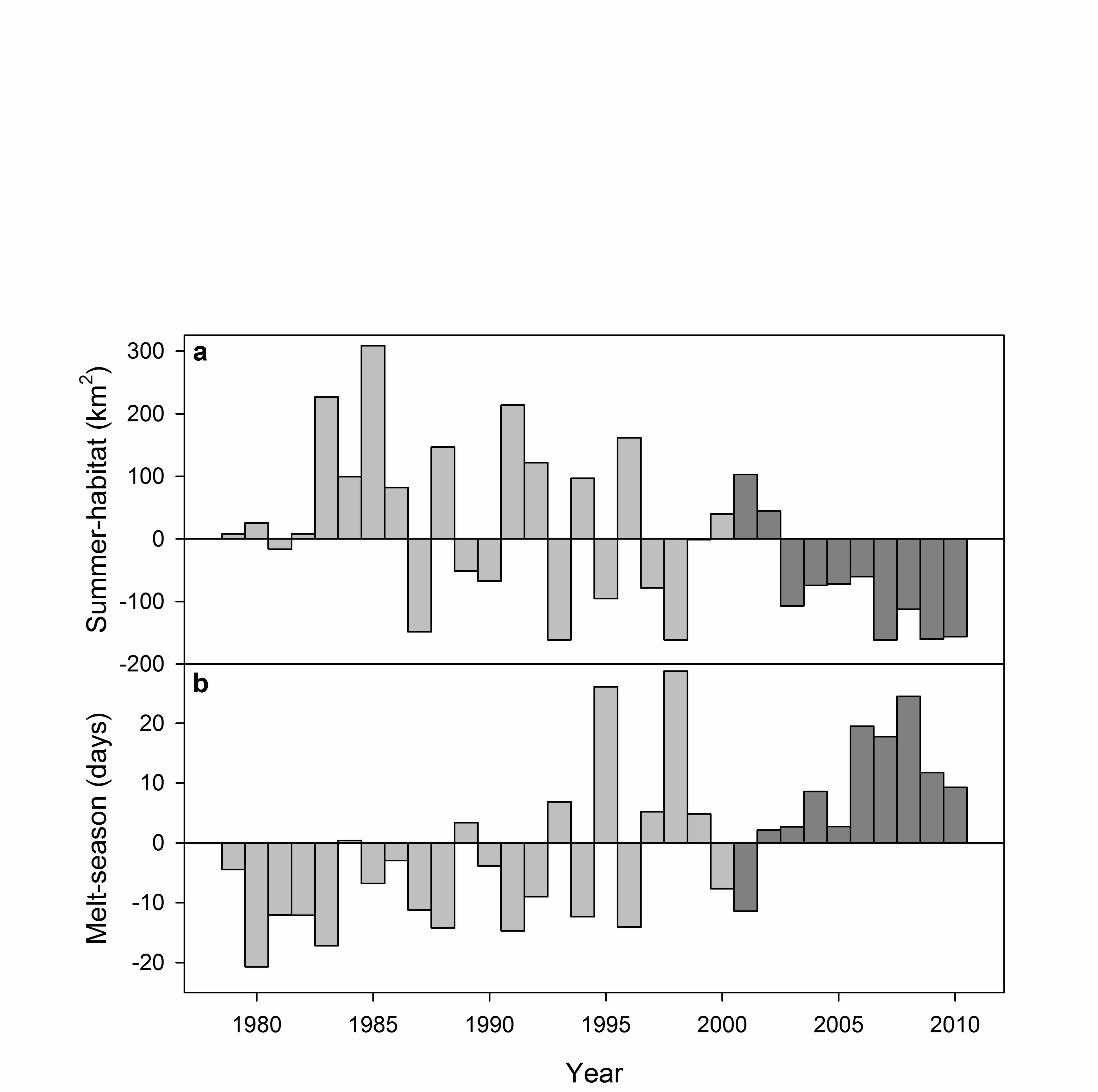
Huggins 2012, Peacock et al. 2013, Thorson et al. 2013). We constructed the ice covariate 208

Summer-habitat by summing monthly indices of the area (km2) of optimal polar bear habitat over 209

the SBS continental shelf (Durner et al. 2009) for July through October of each year (Fig. 2). 210

We expected this covariate to be informative because it was based on the availability of habitat 211

preferred by radio-collared polar bears. The ice covariate Melt-season measured the time 212

between the melt and freeze onset in the Beaufort Sea each summer (Fig. 2; Inner Melt Length; 213

Markus et al. 2009, Stroeve et al. 2014), obtained courtesy of Dr. Julienne Stroeve (National 214

Snow and Ice Data Center, University of Colorado, personal communication). We included 215

Melt-season because it covered a broader geographic region than Summer-habitat and the two 216

covariates were not highly correlated (r = -0.68). The means and standard deviations of the ice 217

covariates from 2001 to 2010 were used to normalize their values before analysis. 218

219

Recapture probability models 220

Recapture models incorporated covariates for sex and the four age classes previously 221

described. We constrained recapture probabilities of cubs and yearlings to equal those of adult 222

females because family groups were captured simultaneously (Age01.3Fem). We constructed a 223

group of time-varying indicator covariates (UA) to model potential discontinuities in Canadian 224

recapture probabilities after 2006, because UA researchers targeted females and subadults and 225

expended less capture effort from 2007 to 2010. 226

Recapture models incorporated two nonparametric forms of temporal structure, either 227

constant through time or a separate probability for each year (Time). In addition, we constructed 228

covariates to model temporal variation arising from heterogeneity in capture effort. The hours 229

11

spent searching for polar bears in the U.S. each year was recorded by USGS (Search-US). The 230

total hours spent flying in Canada was recorded and we assumed 60% of flight hours were spent 231

actively searching for polar bears, a percentage derived from USGS flight records. We added the 232

resulting approximation of Canadian search hours to USGS search hours to construct a measure 233

of effort for the entire study area (Search). In addition, we stratified annual search hours in the 234

U.S. and Canada into low, medium, and high effort categories (Eff-US, Eff-CA), which Stirling et 235

al. (2011) found useful. 236

We incorporated geographic structure into some models because recapture probabilities vary 237

within the study area (Amstrup et al. 2001). We assigned individuals to a home stratum based on 238

the proximity of their mean capture longitude to the four operational bases (Fig. 1), and used 239

stratum assignments to construct four indicator covariates: Barrow, Deadhorse, Barter Island, 240

and Canada (Home). These covariates reflected coarse variation in recapture probabilities 241

among regions, rather than distinct locations as would be used in multi-state models (White et al. 242

2006). We collapsed the Home covariates into two covariates corresponding to country (US, CA) 243

for some models. In addition, we used an indicator covariate (BI2006) to accommodate the lack 244

of effort from the Barter Island base in 2006. 245

Two covariates improved model fit so greatly that we included them in all recapture models. 246

The first (Radio) indicated whether a bear was wearing an active radio during the sampling 247

period each year. Instrumented bears were often targeted for sampling to evaluate their 248

condition and retrieve radios, and could therefore have elevated recapture probabilities; similar 249

covariates have been used by other researchers (e.g., Amstrup et al. 2001, Regehr et al. 2010, 250

Stirling et al. 2011). The second covariate (Cap-procliv) modeled potential recapture 251

heterogeneity unexplained by other covariates, using an individual’s prior capture history as a 252

12

measure of its current tendency to be recaptured (Appendix F), indirectly accounting for 253

individual characteristics, such as behavior, that are difficult to quantify. 254

We constructed models of recapture probability from combinations of four age and sex class 255

effects and eight covariate combinations representing temporal and geographic (abiotic) structure 256

(Table 3, 4). 257

258

Modeling strategies 259

We formed CJS models from combinations of survival and recapture sub-models (Tables 2-260

4). We utilized the plausible combinations (PC) strategy (Bromaghin et al. 2013), with an 261

Akaike’s Information Criterion (AICC) model weight (Burnham and Anderson 2002) of 2.5% as 262

an inclusion threshold, to objectively base inference on a reduced model space. Simulation 263

results (Bromaghin et al. 2013) suggest its performance is similar to that of the “all 264

combinations” strategy recommended by Doherty et al. (2012). 265

We utilized R version 3.0.3. (RCT 2013) for data manipulation and version 2.14 of the R 266

package mra (http://cran.r-project.org/web/packages/mra/index.html) to estimate model 267

parameters (function F.cjs.estim), using the Horvitz-Thompson estimator of abundance (Horvitz 268

and Thompson 1952, McDonald and Amstrup 2001), and compute model-averaged estimates 269

based on AICC model weights (function F.cr.model.avg). 270

We evaluated estimation precision using bootstrap resampling (Chernick 1999), drawing 271

bootstrap samples of capture histories and individual covariates at random with replacement. For 272

each sample, we implemented the PC strategy to select models, estimate the parameters of all 273

selected models, and compute model-averaged estimates (Burnham and Anderson 2002) of 274

recapture, survival, and abundance. Because of the computational burden of this approach, we 275

13

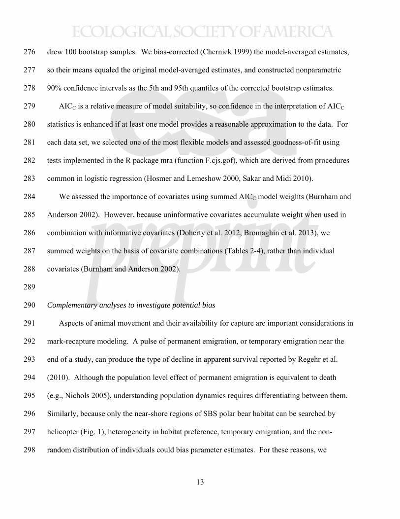
drew 100 bootstrap samples. We bias-corrected (Chernick 1999) the model-averaged estimates, 276

so their means equaled the original model-averaged estimates, and constructed nonparametric 277

90% confidence intervals as the 5th and 95th quantiles of the corrected bootstrap estimates. 278

AICC is a relative measure of model suitability, so confidence in the interpretation of AICC 279

statistics is enhanced if at least one model provides a reasonable approximation to the data. For 280

each data set, we selected one of the most flexible models and assessed goodness-of-fit using 281

tests implemented in the R package mra (function F.cjs.gof), which are derived from procedures 282

common in logistic regression (Hosmer and Lemeshow 2000, Sakar and Midi 2010). 283

We assessed the importance of covariates using summed AICC model weights (Burnham and 284

Anderson 2002). However, because uninformative covariates accumulate weight when used in 285

combination with informative covariates (Doherty et al. 2012, Bromaghin et al. 2013), we 286

summed weights on the basis of covariate combinations (Tables 2-4), rather than individual 287

covariates (Burnham and Anderson 2002). 288

289

Complementary analyses to investigate potential bias 290

Aspects of animal movement and their availability for capture are important considerations in 291

mark-recapture modeling. A pulse of permanent emigration, or temporary emigration near the 292

end of a study, can produce the type of decline in apparent survival reported by Regehr et al. 293

(2010). Although the population level effect of permanent emigration is equivalent to death 294

(e.g., Nichols 2005), understanding population dynamics requires differentiating between them. 295

Similarly, because only the near-shore regions of SBS polar bear habitat can be searched by 296

helicopter (Fig. 1), heterogeneity in habitat preference, temporary emigration, and the non-297

random distribution of individuals could bias parameter estimates. For these reasons, we 298

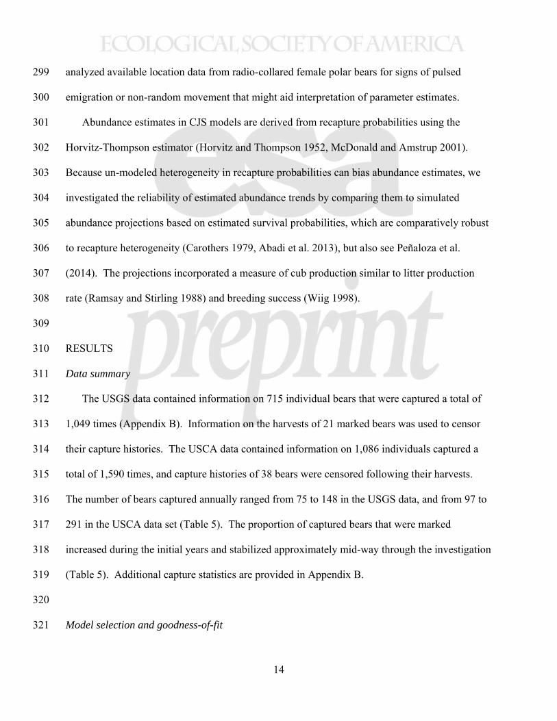
14

analyzed available location data from radio-collared female polar bears for signs of pulsed 299

emigration or non-random movement that might aid interpretation of parameter estimates. 300

Abundance estimates in CJS models are derived from recapture probabilities using the 301

Horvitz-Thompson estimator (Horvitz and Thompson 1952, McDonald and Amstrup 2001). 302

Because un-modeled heterogeneity in recapture probabilities can bias abundance estimates, we 303

investigated the reliability of estimated abundance trends by comparing them to simulated 304

abundance projections based on estimated survival probabilities, which are comparatively robust 305

to recapture heterogeneity (Carothers 1979, Abadi et al. 2013), but also see Peñaloza et al. 306

(2014). The projections incorporated a measure of cub production similar to litter production 307

rate (Ramsay and Stirling 1988) and breeding success (Wiig 1998). 308

309

RESULTS 310

Data summary 311

The USGS data contained information on 715 individual bears that were captured a total of 312

1,049 times (Appendix B). Information on the harvests of 21 marked bears was used to censor 313

their capture histories. The USCA data contained information on 1,086 individuals captured a 314

total of 1,590 times, and capture histories of 38 bears were censored following their harvests. 315

The number of bears captured annually ranged from 75 to 148 in the USGS data, and from 97 to 316

291 in the USCA data set (Table 5). The proportion of captured bears that were marked 317

increased during the initial years and stabilized approximately mid-way through the investigation 318

(Table 5). Additional capture statistics are provided in Appendix B. 319

320

Model selection and goodness-of-fit 321

15

The PC model selection strategy (Bromaghin et al. 2013) with the USGS data resulted in the 322

retention of 60 survival probability models and 20 recapture probability models. The estimation 323

algorithm failed to converge for one combination of survival and recapture models (Survival: Int 324

+ Age3*Melt-season + Age3Fem + Age2*Melt-season + Age2Fem + Age1*Melt-season + 325

Age0*TS-sur; Recapture: Time + Age01.23.Fems + Radio + Cap-procliv). The model selected to 326

evaluate goodness-of-fit contained 34 parameters (covariate structures listed in bold font in 327

Tables 2 and 3). The results of goodness-of-fit tests did not raise concerns regarding inadequate 328

model fit. The Osius-Rojek test could not be evaluated (it returned a “not-a-number” code), but 329

the Hosmer-Lemeshow test was not significant (p=0.690) and the Receiver Operating 330

Characteristic (ROC) curve displayed acceptable discrimination (0.736). 331

For the USCA data, the PC model selection strategy resulted in 47 survival probability 332

models and 4 recapture probability models being selected for further consideration. The model 333

selected to assess goodness-of-fit contained 39 parameters (covariate structures listed in bold 334

font in Tables 2 and 4). Based on that model, the Osius-Rojek test was moderately significant 335

(p=0.036), but the Hosmer-Lemeshow test was not (p=0.276) and the Receiver Operating 336

Characteristic (ROC) curve displayed acceptable discrimination (0.727), providing no 337

compelling evidence of inadequate model fit. 338

339

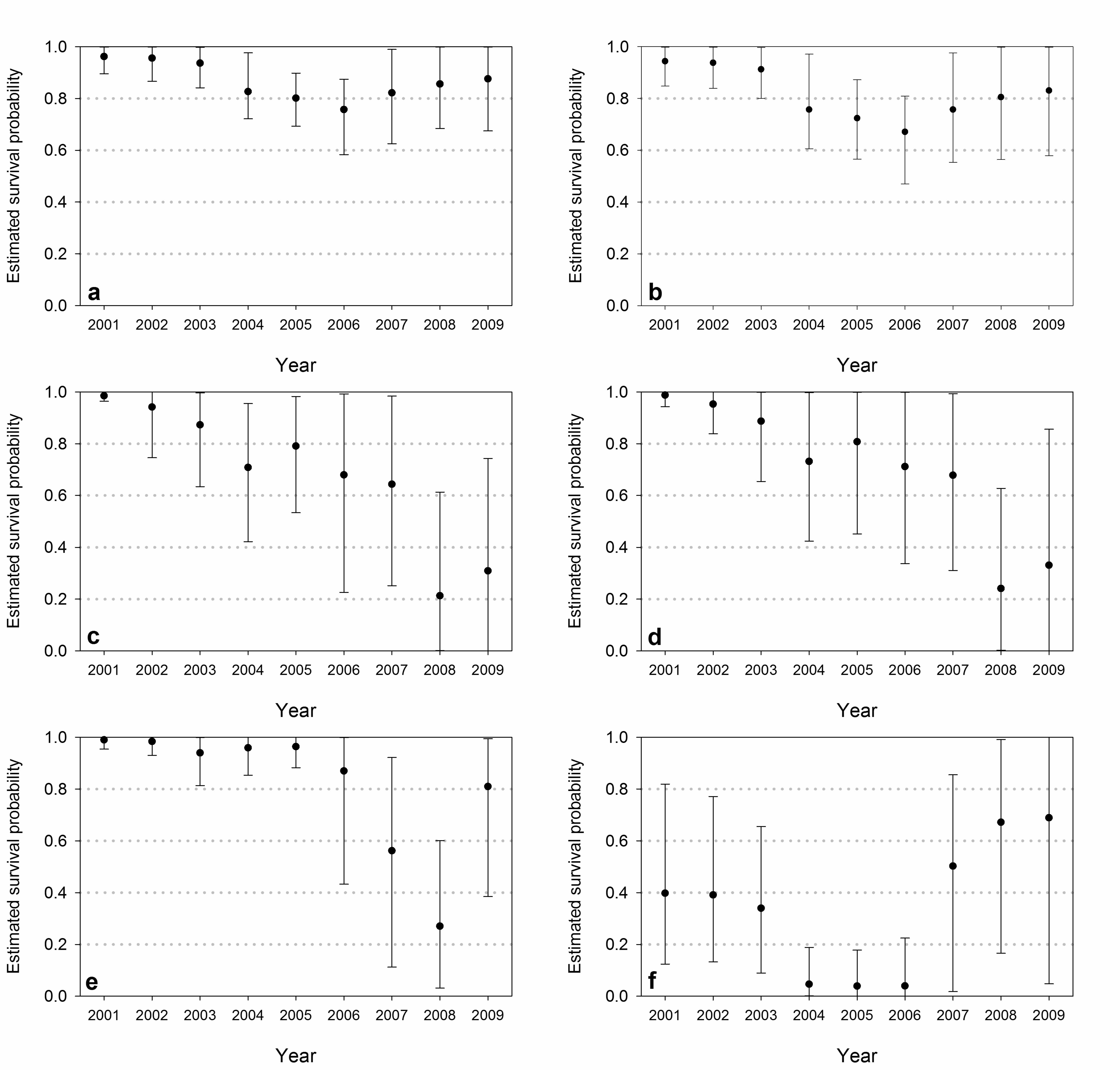
Survival and recapture probabilities 340

Model-averaged estimates of survival based on the USGS data differed among age classes 341

and varied through time (Fig. 3, Table 6). Survival of adult bears was high from 2001 through 342

2003, substantially reduced from 2004 through 2007, and higher but below historical levels in 343

2008 and 2009 (Amstrup and Durner 1995; Amstrup et al. 2001). Point estimates for males were 344

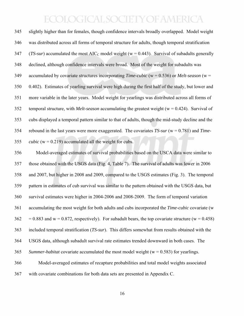
16

slightly higher than for females, though confidence intervals broadly overlapped. Model weight 345

was distributed across all forms of temporal structure for adults, though temporal stratification 346

(TS-sur) accumulated the most AICC model weight (w = 0.443). Survival of subadults generally 347

declined, although confidence intervals were broad. Most of the weight for subadults was 348

accumulated by covariate structures incorporating Time-cubic (w = 0.536) or Melt-season (w = 349

0.402). Estimates of yearling survival were high during the first half of the study, but lower and 350

more variable in the later years. Model weight for yearlings was distributed across all forms of 351

temporal structure, with Melt-season accumulating the greatest weight (w = 0.424). Survival of 352

cubs displayed a temporal pattern similar to that of adults, though the mid-study decline and the 353

rebound in the last years were more exaggerated. The covariates TS-sur (w = 0.781) and Time-354

cubic (w = 0.219) accumulated all the weight for cubs. 355

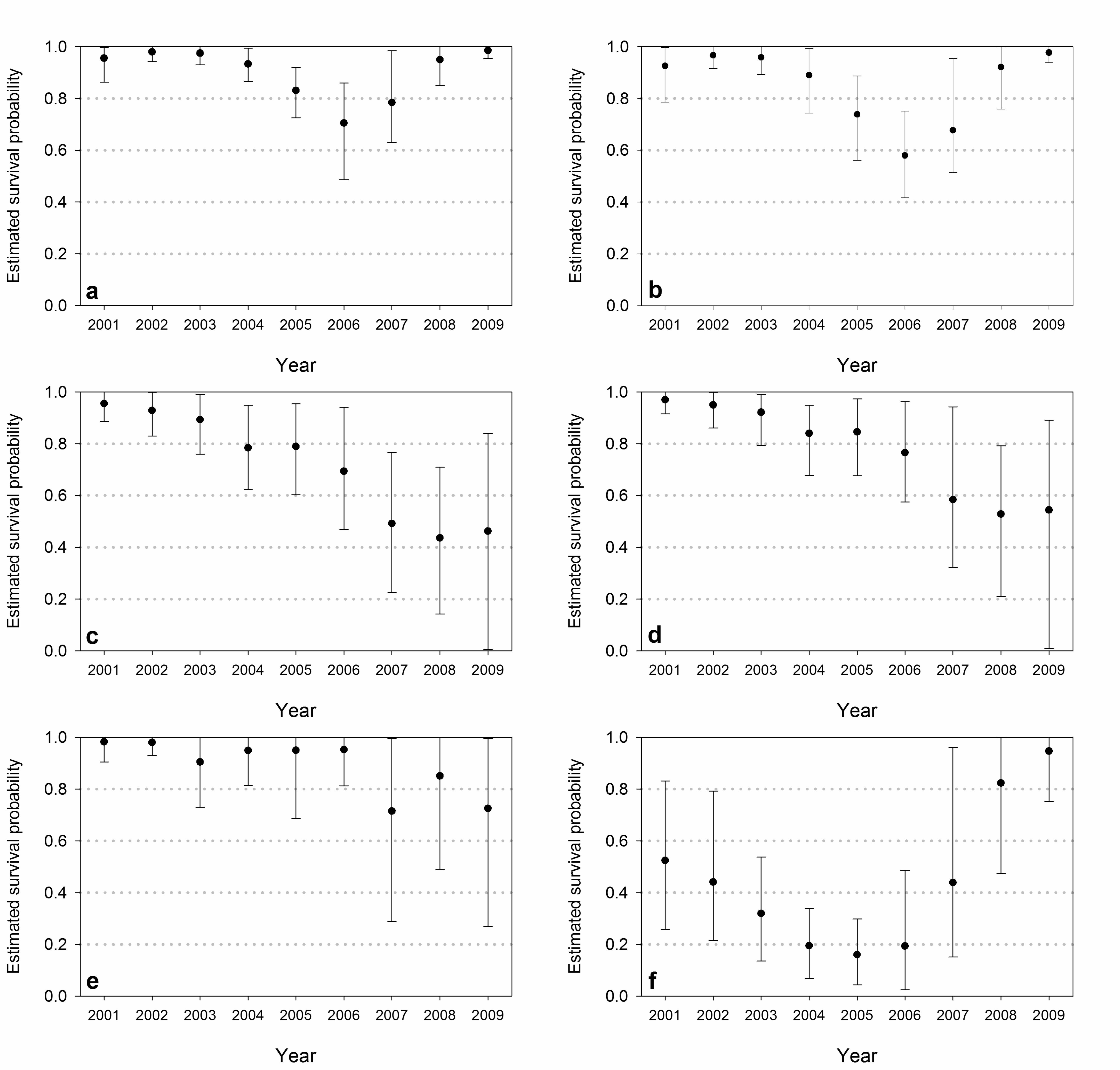
Model-averaged estimates of survival probabilities based on the USCA data were similar to 356

those obtained with the USGS data (Fig. 4, Table 7). The survival of adults was lower in 2006 357

and 2007, but higher in 2008 and 2009, compared to the USGS estimates (Fig. 3). The temporal 358

pattern in estimates of cub survival was similar to the pattern obtained with the USGS data, but 359

survival estimates were higher in 2004-2006 and 2008-2009. The form of temporal variation 360

accumulating the most weight for both adults and cubs incorporated the Time-cubic covariate (w 361

= 0.883 and w = 0.872, respectively). For subadult bears, the top covariate structure (w = 0.458) 362

included temporal stratification (TS-sur). This differs somewhat from results obtained with the 363

USGS data, although subadult survival rate estimates trended downward in both cases. The 364

Summer-habitat covariate accumulated the most model weight (w = 0.583) for yearlings. 365

Model-averaged estimates of recapture probabilities and total model weights associated 366

with covariate combinations for both data sets are presented in Appendix C. 367

17

368

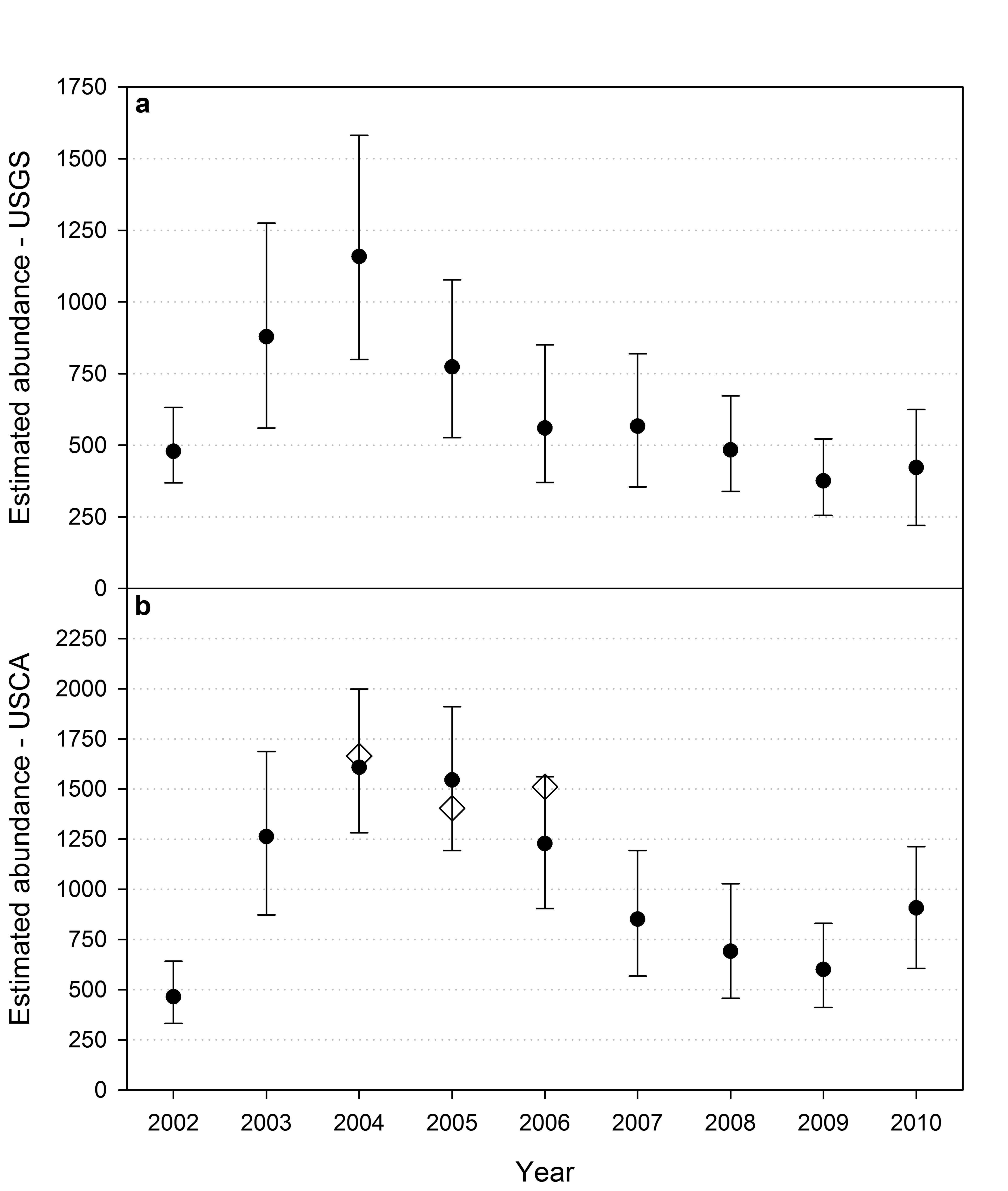
Abundance 369

Annual abundance estimates based on the USGS data, applicable to the Alaskan portion of 370

the study area, ranged from 376 in 2009 to 1,158 in 2004 (Fig. 5a). We suspect estimates in the 371

first two years, particularly 2002, were negatively biased by the absence of capture effort from 372

Barrow in 2001, which may have caused an over-estimate of recapture probability in 2002 373

(Appendix C, Fig. C1-C3). In addition, the mixing of marked and unmarked individuals may 374

have been incomplete during the initial years of the study (Appendix D, Fig. D2). The unusually 375

large number of bears captured in 2004 (Table 5) produced a seemingly large estimate with a 376

wide confidence interval. Even though there is uncertainty regarding abundance levels in these 377

years, the broader pattern of a decline in abundance during the middle of the study followed by 378

relative stability at the end of the study was consistent with patterns in survival. 379

Abundance estimates based on the USCA data ranged from 464 in 2002 to 1,607 in 2004 380

(Fig. 5b). As with the USGS data, we suspect estimates for the initial years of the investigation 381

were less reliable than those in the latter years, particularly because no capture effort occurred in 382

Canada before 2003 and our models were not robust to this deficiency. Considering this 383

uncertainty in the earliest estimates, the temporal pattern in abundance resembled that of the 384

USGS estimates and was consistent with patterns in survival. The correlation between USGS 385

and USCA abundance estimates was 0.84 across all years and 0.86 excluding 2002. 386

387

Complementary analyses to investigate potential bias 388

Analyses of location data from radio-collared females produced no strong evidence that 389

temporary emigration or non-random movement negatively biased estimates of survival 390

18

(Appendix D). An exact test of the hypothesis that equal proportions of collared bears were 391

available for capture each year was not significant (P = 0.990), implying that a pulse of 392

permanent emigration did not occur in the middle of the investigation. We did, however, find 393

indications of non-random movement between near-shore and offshore habitats among 394

consecutive years. Although such non-random movement can bias estimates of recapture and 395

survival probabilities, our data are consistent with conditions in which bias in survival 396

probabilities is small (modest state transition probabilities; Kendall et al. 1997, Schaub et al. 397

2004). 398

The results of population projections were largely consistent with the estimated trends in 399

abundance (Appendix E). Projected abundance increased during the initial years of the study, 400

though more slowly than suggested by the abundance estimates, supporting our conjecture that 401

abundance estimates in the earliest years were negatively biased. Projected abundance declined 402

through the middle of the study and then stabilized. The correlation between abundance 403

estimates and the projections based on the USGS data set was 0.85 across all years and 0.90 404

excluding 2002; the corresponding correlations for the USCA data set were 0.89 and 0.95. 405

406

DISCUSSION 407

Methodological effectiveness 408

We constructed covariates to account for multiple sources of heterogeneity in recapture 409

probabilities that could otherwise bias survival and abundance estimates (Abadi et al. 2013). 410

Recapture probabilities were allowed to vary by sex and age class. Covariates indexed both 411

capture effort and nonparametric temporal structure, and geographic covariates accounted for 412

previously-discovered regional differences in recapture probabilities (Amstrup et al. 2001). The 413

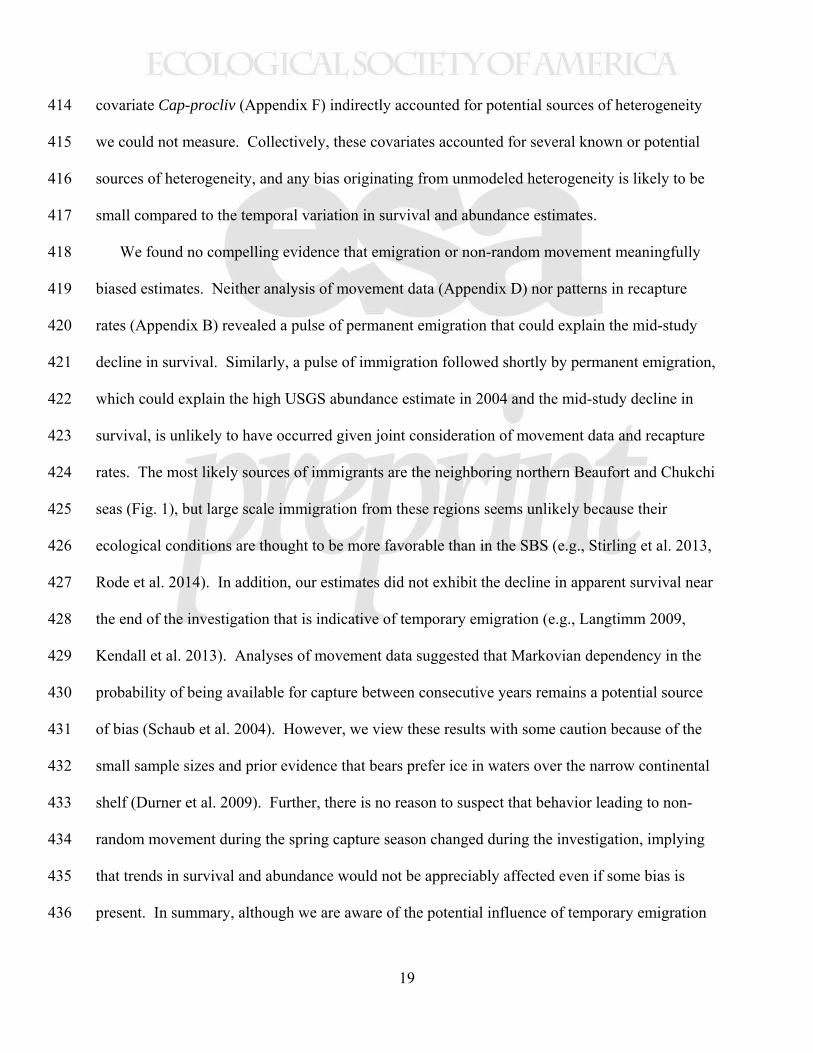
19

covariate Cap-procliv (Appendix F) indirectly accounted for potential sources of heterogeneity 414

we could not measure. Collectively, these covariates accounted for several known or potential 415

sources of heterogeneity, and any bias originating from unmodeled heterogeneity is likely to be 416

small compared to the temporal variation in survival and abundance estimates. 417

We found no compelling evidence that emigration or non-random movement meaningfully 418

biased estimates. Neither analysis of movement data (Appendix D) nor patterns in recapture 419

rates (Appendix B) revealed a pulse of permanent emigration that could explain the mid-study 420

decline in survival. Similarly, a pulse of immigration followed shortly by permanent emigration, 421

which could explain the high USGS abundance estimate in 2004 and the mid-study decline in 422

survival, is unlikely to have occurred given joint consideration of movement data and recapture 423

rates. The most likely sources of immigrants are the neighboring northern Beaufort and Chukchi 424

seas (Fig. 1), but large scale immigration from these regions seems unlikely because their 425

ecological conditions are thought to be more favorable than in the SBS (e.g., Stirling et al. 2013, 426

Rode et al. 2014). In addition, our estimates did not exhibit the decline in apparent survival near 427

the end of the investigation that is indicative of temporary emigration (e.g., Langtimm 2009, 428

Kendall et al. 2013). Analyses of movement data suggested that Markovian dependency in the 429

probability of being available for capture between consecutive years remains a potential source 430

of bias (Schaub et al. 2004). However, we view these results with some caution because of the 431

small sample sizes and prior evidence that bears prefer ice in waters over the narrow continental 432

shelf (Durner et al. 2009). Further, there is no reason to suspect that behavior leading to non-433

random movement during the spring capture season changed during the investigation, implying 434

that trends in survival and abundance would not be appreciably affected even if some bias is 435

present. In summary, although we are aware of the potential influence of temporary emigration 436

20

and non-random movement, we believe any bias from these sources is likely to be small 437

compared to the magnitude of temporal variation and trends in survival and abundance estimates. 438

We believe that the assumptions of the Horvitz-Thompson abundance estimator (Horvitz and 439

Thompson 1952, McDonald and Amstrup 2001) were satisfied. As previously discussed, 440

covariates were utilized to model several known and potential sources of heterogeneity in 441

recapture probabilities, so there is no reason to suspect they are systematically biased. The CJS 442

model conditions on initial captures and estimates subsequent recapture probabilities, while the 443

Horvitz-Thompson estimator applies estimated recapture probabilities to both initial captures and 444

recaptures (McDonald and Amstrup 2001). A behavioral response to initial capture that lowers 445

recapture probabilities therefore has the potential to positively bias abundance estimates. 446

However, our capture methods largely preclude such a behavioral response. Bears are often 447

located by following fresh tracks in snow. There are patches of rough ice in which bears could 448

attempt to hide, if they were not being tracked, but we have not observed hiding behavior. Most 449

bears move away as the helicopter approaches, though some display curiosity or aggression 450

toward it. In addition, we are unaware of any information that suggests our abundance estimates 451

are unrealistically high. 452

453

Insights into ecological mechanisms 454

The previously reported low survival of SBS polar bears in 2004 and 2005 (Regehr et al. 455

2010) continued into 2007, at levels substantially less than earlier estimates for this population 456

(Amstrup and Durner 1995, Amstrup et al. 2001). Annual survival of cubs during that period 457

was estimated to be less than 0.2 based on the USCA data and near zero with the USGS data. 458

Indeed, only 2 of 80 cubs in the USGS data observed from 2003 to 2007 are known to have 459

21

survived to an older age class (Appendix B, Fig. B1). Such poor recruitment, combined with 460

reduced survival of other age classes, must have substantially impacted abundance, and our 461

abundance estimates declined accordingly during those years. Estimated survival of adults and 462

cubs from both data sets began to improve in 2007, with estimates based on the USCA data 463

suggesting a somewhat stronger recovery, although confidence intervals overlap broadly. This 464

potential divergence may be an early indication of regional differences in ecosystem function 465

and polar bear response that may become more apparent as the Arctic continues to warm. 466

Several independent sources of information are consistent with reduced survival during the 467

middle of the study period. Cherry et al. (2009) found physiological indications of nutritional 468

stress to be two to three times greater in 2005 and 2006 than in the 1980s. Regehr et al. (2006) 469

reported observations of starvation during this period, and unusual incidents of polar bears 470

stalking and killing other bears occurred in 2004 (Amstrup et al. 2006). Stirling et al. (2008) 471

reported a case of cannibalism and several instances of polar bears penetrating unusually thick 472

ice barriers to reach ringed seal lairs between 2003 and 2007, predatory behavior that is 473

energetically inefficient and a likely indication of nutritional stress. A similar instance of ice 474

penetration was observed in the SBS in 1975 (Stirling et al. 2008), during a period of low seal 475

production and reduced polar bear cub survival throughout the Canadian portion of the Beaufort 476

Sea (Stirling 2002). Similar low productivity of ringed seals and reduced survival of polar bear 477

cubs were documented in the Canadian portion of the Beaufort Sea again in the mid-1980s 478

(Smith 1987; Stirling 2002). 479

Factors leading to improved survival beginning in 2007 are difficult to identify, but there are 480

indications of a transition at this time. Pilfold et al. (2014) reported a shift in the distribution of 481

seal kill sites among land-fast and pack ice between the periods 2003-2006 and 2007-2011, and 482

22

more kill sites were located in the latter period. The pattern and occurrence of open-water lead 483

systems and ice deformation within the central Beaufort Sea changed in 2006 (Mahoney et al. 484

2012). Similarly, Melling et al. (2012) reported unusual atmospheric and oceanographic 485

conditions in the Beaufort Sea during 2007. Ringed seal productivity within Amundsen Gulf in 486

the eastern SBS was low in 2005 and 2006, but improved in 2007 (Harwood et al. 2012), 487

although this was attributed to localized ice conditions and is not thought to be indicative of the 488

low ringed seal production broadly observed in the 1970s and 1980s (Stirling 2002). Potential 489

linkages between these indicators of a transition in the 2006-2007 timeframe and polar bear 490

survival may become apparent as our understanding of Arctic ecology improves. 491

Improved survival after 2007 might be partially attributable to either density dependent 492

mechanisms or the altered characteristics or behavior of surviving individuals. Reduced 493

competition for limited resources resulting from lower abundance may have increased survival at 494

the end of the study period. Similarly, consecutive years of unfavorable conditions may have 495

eliminated the less fit individuals from the population, with the survivors collectively displaying 496

seemingly enhanced survival. Finally, some individuals may have adopted behavior that 497

increased their survival. For example, a growing proportion of the population utilizes terrestrial 498

habitat after ice retreats from the continental shelf in summer (USGS unpublished data). These 499

bears have access to subsistence-harvested bowhead whale carcasses at discrete locations along 500

the Alaskan coast (Herreman and Peacock 2013), an energy-rich alternative food source 501

(Bentzen et al. 2007) that may enhance survival. Bears utilizing terrestrial habitat in summer 502

may also have earlier access to seals in autumn. Land-fast ice begins to form over coastal waters 503

earlier than the expanding pack ice provides bears summering on perennial ice deep in the Polar 504

23

Basin with access to continental shelf waters. Such behavioral tendencies are likely to be 505

adopted by dependent young and may therefore become increasingly common. 506

Subadults, unlike adults and cubs, did not display increased survival during the latter years of 507

our investigation. Newly independent and inexperienced individuals are likely to be less 508

efficient hunters, and less capable of competing for limited resources or retaining control of kills, 509

than adults (Stirling 1974), and may be more susceptible to unfavorable conditions. Subadults 510

are also less likely to utilize crowded feeding sites such as bowhead whale remains. Sea ice 511

covariates were more strongly associated with the survival of subadults than adults, which is 512

consistent with findings that the body condition of growing bears is more closely linked to ice 513

conditions than that of older bears (Rode et al. 2010). The lack of an improvement in subadult 514

survival may be, in part, a residual effect of poor conditions in prior years. Yearlings that 515

survived to subadult status during years of low survival may have been in inadequate condition 516

to survive independently. Regardless of cause, the status of subadults in the SBS population 517

merits monitoring, because their continued low survival could ultimately lead to further declines 518

in abundance. 519

Polar bears depend on sea ice for several aspects of their life history and multiple 520

characteristics of sea ice can be expected to influence their vital rates, potentially via 521

mechanisms that are complex and nonlinear (e.g., Ellis and Post 2004, Tyler et al. 2008, 522

Derocher et al. 2013). The duration of ice-absence from the continental shelf is thought to 523

directly affect polar bear condition and vital rates through reduced access to prey (Rode et al. 524

2010, Regehr et al. 2010, Rode et al. 2012). Observations of polar bears and seal kills in low- 525

concentration, unconsolidated ice (unpublished field observations: Chukchi Sea in 2009, SBS in 526

2010) testify to the high value of sea ice in biologically productive shelf waters. However, other 527

24

aspects of sea ice are undoubtedly important. Extensive ice rubble and rafted floes during winter 528

and spring are thought to have led to past declines in polar bear productivity in the SBS (Stirling 529

et al. 1976, Amstrup et al. 1986, Stirling 2002), as well as during our investigation (Stirling et al. 530

2008). The increased frequency and severity of storms (Sepp and Jaagus 2011, Thomson and 531

Rodgers 2014) combined with thinner and more mobile pack ice (Spreen et al. 2011), both 532

consequences of climate warming, are likely to result in a greater prevalence of deformed ice in 533

winter and spring that may result in lower quality ringed seal birth lair habitat and subsequent 534

reductions in reproductive success. Similarly, continued warming may increase the frequency 535

of unsuitable snow and ice conditions for maintenance of ringed seal lairs (Stirling and Smith 536

2004, Hezel et al. 2012). The increased vulnerability of ringed seal pups to predation could 537

temporarily enhance polar bear survival, though it would likely also lead to subsequent 538

reductions in prey abundance. Finally, access to terrestrial denning sites can be limited by ice 539

conditions (Derocher et al. 2011). 540

Despite the known importance of sea ice, measures of ice availability did not fully explain 541

short-term demographic patterns in our data, suggesting that other aspects of the ecosystem 542

contribute importantly to the regulation of population dynamics. Prey abundance can obviously 543

affect bear condition and survival independently, to an extent, of sea ice conditions. Numerous 544

factors such as warming-induced increases in primary productivity (Zhang et al. 2010), 545

phenology-based trophic mismatches (Post et al. 2013), changing disease vectors (Jensen et al. 546

2010), increased contaminant transport (Sonne 2010), and expanding human activity in the 547

Arctic (Smith and Stephenson 2013) may interact with the primary effects of sea ice conditions 548

and prey accessibility. As the Arctic continues to warm, ecosystem structure and function can be 549

expected to respond (e.g., Lasternas and Agusti 2010, Carroll et al. 2013, Hezel et al. 2012, 550

25

Hinzman et al. 2013, Ji et al. 2013, Iverson et al. 2014, Nahrgang et al. 2014), perhaps in ways 551

that are difficult to foresee. Although sea ice availability is expected to be the dominant driver of 552

population dynamics over the long term (Amstrup et al. 2008, Stirling and Derocher 2012), other 553

aspects of the ecosystem can be expected to either mitigate or exacerbate the effects of sea ice 554

loss in the short term. The changing Arctic ecosystem may induce increased short term variation 555

in vital rates and elevate the risk of abrupt population decline (Derocher et al. 2013). 556

557

Conclusions 558

Our results collectively suggest that polar bears in the SBS experienced a significant 559

reduction in survival and abundance from 2004 through 2007. However, suspected biases in the 560

abundance estimates for the earliest years of the investigation, potential biases in the USCA 561

estimates in the latter years, and statistical variation associated with estimates necessitate 562

cautious expression of the magnitude of population decline. Conservatively, the decline seems 563

unlikely to have been less than 25%, but may have approached 50%. Improved survival and 564

stability in abundance at the end of the investigation are cause for cautious optimism. However, 565

given projections for continued climate warming (IPCC 2013), polar bear ecology in the SBS 566

and elsewhere in the Arctic is expected to become increasingly forced by sea ice loss (Amstrup 567

et al. 2008, Stirling and Derocher 2012). Behavioral plasticity and ecosystem productivity may 568

enable some populations to temporarily maintain recruitment and abundance, despite 569

deteriorating habitat conditions (e.g., Rode et al. 2014), but seem unlikely to counterbalance the 570

extensive habitat degradation projected to occur over the long term (IPCC 2013). Continued 571

research into the ecological mechanisms underlying polar bear population dynamics is necessary 572

26

to refine projections of their future status and develop appropriate strategies for their 573

management. 574

575

ACKNOWLEDGEMENTS 576

We thank the many members of the U.S. Geological Survey, Environment Canada, and the 577

University of Alberta field crews and the pilots transporting them for collection of the raw data. 578

We also thank Dr. Julienne Stroeve of the University of Colorado, National Snow and Ice Data 579

Center for providing the melt-season covariate, and Tom Evans, U.S. Fish and Wildlife Service, 580

Marine Mammals Management, Anchorage, Alaska, and Marsha Branigan, Government of the 581

Northwest Territories, Environment and Natural Resources, Inuvik, NT for providing access to 582

harvest records of marked bears. William Kendall, Karen Oakley, Karyn Rode, and Michael 583

Runge of the U.S. Geological Survey, and five anonymous referees provided helpful comments 584

on earlier drafts. The Subject Matter Editor’s management of peer review was extremely 585

helpful. Support for long-term research on SBS polar bears conducted in the U.S. was provided 586

by U.S. Geological Survey, Ecosystems and Climate and Land Use Change Mission Areas and 587

the U.S. Bureau of Land Management. Support for research conducted in Canada was provided 588

by the Canadian Wildlife Federation; Environment Canada; Circumpolar/ Boreal Alberta 589

Research; Inuvialuit Game Council; National Fish and Wildlife Federation; Natural Sciences and 590

Engineering Research Council of Canada; Northern Scientific Training Program; Northwest 591

Territories Department of Environment and Natural Resources; Parks Canada; Polar Bears 592

International; Polar Continental Shelf Project; Quark Expeditions; U.S. Bureau of Ocean Energy 593

Management; U.S. Geological Survey, Ecosystems Mission Area, Science Support Partnership 594

Program (2003-2005); University of Alberta; and World Wildlife Fund (Canada). The findings 595

27

and conclusions in this article are those of the authors and do not necessarily represent the views 596

of the U.S. Fish and Wildlife Service (EVR). Any mention of trade names is for descriptive 597

purposes only and does not constitute endorsement by the U.S. federal government. 598

599

LITERATURE CITED 600

Abadi, F., A. Botha, and R. Altwegg. 2013. Revisiting the effect of capture heterogeneity on 601

survival estimates in capture-mark-recapture studies: Does it matter? PLoS ONE 8:e62636. 602

Amstrup, S. C., E. T. DeWeaver, D. C. Douglas, B. G. Marcot, G. M. Durner, C. M. Bitz, and D. 603

A. Bailey. 2010. Greenhouse gas mitigation can reduce sea-ice loss and increase polar bear 604

persistence. Nature 468:955-958. 605

Amstrup, S. C., and G. M. Durner. 1995. Survival rates of radio-collared female polar bears and 606

their dependent young. Canadian Journal of Zoology 73:1312-1322. 607

Amstrup, S. C., and C. Gardner. 1994. Polar bear maternity denning in the Beaufort Sea. Journal 608

of Wildlife Management 58:1-10. 609

Amstrup, S. C., B. G. Marcot, and D. C. Douglas. 2008. A Bayesian network modeling approach 610

to forecasting the 21st century worldwide status of polar bears. Pages 213-268 in E. T. 611

DeWeaver, C. M. Bitz, and L.-B. Tremblay, editors. Arctic sea ice decline: Observations, 612

projections, mechanisms, and Implications. Geophysical Monograph Series 180. American 613

Geophysical Union, Washington, D. C. 614

Amstrup, S. C., T. L. McDonald, B. F. J. Manly. 2005. Handbook of capture-recapture analysis. 615

Princeton University Press. Princeton, New Jersey. 616

28

Amstrup, S. C., T. L. McDonald, and I. Stirling. 2001. Polar bears in the Beaufort Sea: A 30-year 617

mark-recapture case history. Journal of Agricultural, Biological, and Environmental Statistics 618

6:221-234. 619

Amstrup, S. C., I. Stirling, J. W. Lentfer. 1986. Past and present status of polar bears in Alaska. 620

Wildlife Society Bulletin 14:241-254. 621

Amstrup, S.C., I. Stirling, T. S. Smith, C. Perham, and G. W. Thiemann. 2006. Recent 622

observations of intraspecific predation and cannibalism among polar bears in the southern 623

Beaufort Sea. Polar Biology 29:997-1002. 624

Ashjian, C. J., S. R. Braund, R. G. Campbell, J. C. George, J. Kruse, W. Maslowski, S. E. 6 625

Moore, C. R. Nicolsoson, S. R. Okkonen, B. F. Sherr, E. B. Sherr, and Y. H. Spitz. 2010. 626

Climate variability, oceanography, bowhead whale distribution, and Iñupiat subsistence 627

whaling near Barrow, Alaska. Arctic 63:179-194. 628

Banašek-Richter, C., L. Bersier, M. Cattin, R. Baltensperger, J. Gabriel, Y. Merz, R. E. 629

Ulanowicz, A. F. Tavares, D. D. Williams, P. C. Ruiter, K. O. Winemiller, and R. E. Naisbit. 630

2009. Complexity in quantitative food webs. Ecology 90:1470-1477. 631

Bentzen, T. W., E. H. Follmann, S. C. Amstrup, G. S. York, M. J. Wooller, and T. M. O'Hara. 632

2007. Variation in winter diet of southern Beaufort Sea polar bears inferred from stable 633

isotope analysis. Canadian Journal of Zoology 85:596-608. 634

Bromaghin, J. F., T. L. McDonald, and S. C. Amstrup. 2013. Plausible combinations: An 635

improved method to evaluate the covariate structure of Cormack-Jolly-Seber mark-recapture 636

models. Open Journal of Ecology 3:11-22. 637

Burnham, K. P., and D. R. Anderson. 2002. Model selection and multimodel inference: a 638

practical information-theoretic approach. Springer-Verlag, New York, New York, USA. 639

29

Carothers, A. D. 1979. Quantifying unequal catchability and its effect on survival estimates in an 640

actual population. Journal of Animal Ecology 48:863-869. 641

Carroll, S. S., L. Horstmann-Dehn, and B. L. Norcross. 2013. Diet history of ice seals using 642

stable isotope ratios in claw growth bands. Canadian Journal of Zoology 91:191-202. 643

Chernick, M. R. 1999. Bootstrap methods: A practitioner’s guide. John Wiley & Sons, New 644

York, New York, USA. 645

Cherry, S. G., A. E. Derocher, K. A. Hobson, I. Stirling, and G. W. Thiemann. 2011. Quantifying 646

dietary pathways of proteins and lipids to tissues of a marine predator. Journal of Applied 647

Ecology 48:373-381. 648

Cherry, S. G., A. E. Derocher, I. Stirling, and E. S. Richardson. 2009. Fasting physiology of 649

polar bears in relation to environmental change and breeding behavior in the Beaufort Sea. 650

Polar Biology 32:383-391. 651

Derocher, A. E., J. Aars, S. C. Amstrup, A. Cutting, N. J. Lunn, P. K. Molnár, M. E. Obbard, I. 652

Stirling, G. W. Thiemann, D. Vongraven, Ø. Wiig, and G. York. 2013. Rapid ecosystem 653

change and polar bear conservation. Conservation Letters. DOI 10.1111/conl.12009. 654

Derocher, A. E., M. Andersen, Ø. Wiig, A. Aars, E. Hansen, and M. Biuw. 2011. Sea ice and 655

polar bear den ecology at Hopen Island, Svalbard. Marine Ecology Progress Series 441:273-656

279. 657

Doherty, P., G. White, and K. Burnham. 2012. Comparison of model building and selection 658

strategies. Journal of Ornithology 152:317-323. 659

Dunton, K. H., T. Weingartner, and E. C. Carmack. 2006. The nearshore western Beaufort Sea 660

ecosystem: Circulation and importance of terrestrial carbon in arctic coastal food webs. 661

Progress in Oceanography 71:362-378. 662

30

Durner, G. M., D. C. Douglas, R. M. Nielson, S. C. Amstrup, T. L. McDonald, I. Stirling, M. 663

Mauritzen, E. W. Born, Ø. Wiig, E. DeWeaver, M. C. Serreze, S. E. Belikov, M. M. Holland, 664

J. Maslanik, J. Aars, D. A. Bailey, and A. E. Derocher. 2009. Predicting 21st-century polar 665

bear habitat distribution from global climate models. Ecological Monographs 79:25-58. 666

Durner, G. M., J. P. Whiteman, H. J. Harlow, S. C. Amstrup, E. V. Regehr, and M. Ben-David. 667

2011. Consequences of long-distance swimming and travel over deep-water pack ice for a 668

female polar bear during a year of extreme sea ice retreat. Polar Biology 34:975-984. 669

Ellis, A. M., and E. Post. 2004. Population response to climate change: Linear vs. non-linear 670

modeling approaches. BMC Ecology 4:2. 671

Fischbach, A. S., S. C. Amstrup, and D. C. Douglas. 2007. Landward and eastward shift of 672

Alaskan polar bear denning associated with recent sea ice changes. Polar Biology 30:1395-673

1405. 674

Frost, K. J., L. F. Lowry, G. Pendleton, and H. R. Nute. 2004. Factors affecting the observed 675

densities of ringed seals, Phoca hispida, in the Alaskan Beaufort Sea, 1996–99. Arctic 676

57:115-128. 677

Giles, K. A., S. W. Laxon, A. L. Ridout, D. J. Wingham, and S. Bacon. 2012. Western Arctic 678

Ocean freshwater storage increased by wind-driven spin-up of the Beaufort Gyre. Nature 679

Geoscience 5:194-197. 680

Grebmeier, J. M., L. W. Cooper, H. M. Feder, and B. I. Sirenko. 2006. Ecosystem dynamics of 681

the pacific-influenced northern Bering and Chukchi seas in the Amerasian Arctic. Progress in 682

Oceanography 71:331-361. 683

31

Harwood, L. A., T. G. Smith, H. Melling, J. Alikamik, and M. C. S. Kingsley. 2012. Ringed 684

seals and sea ice in Canada’s Western Arctic: harvest-based monitoring 1992-2011. Arctic 685

65:377-390. 686

Herreman, J., and E. Peacock. 2013. Polar bear use of a persistent food subsidy: Insights from 687

non-invasive genetic sampling in Alaska. Ursus 24:148-163. 688

Hezel, P. J., X. Zhang, C. M. Bitz, B. P. Kelly, and F. Massonnet. 2012. Projected decline in 689

spring snow depth on Arctic sea ice caused by progressively later autumn open ocean freeze-690

up this century. Geophysical Research Letters 39:17505. 691

Hinzman, L. D., C. J. Deal, A. D. McGuire, S. H. Mernild, I. V. Polyakov, and J. E. Walsh. 692

2013. Trajectory of the Arctic as an integrated system. Ecological Applications 23:1837-693

1868. 694

Horner, R., and G. C. Schrader. 1982. Relative contributions of ice algae, phytoplankton, and 695

benthic microalgae to primary production in nearshore regions of the Beaufort Sea. Arctic 696

35:485-503. 697

Horvitz, D. G., and D. J. Thompson. 1952. A generalization of sampling without replacement 698

from a finite universe. Journal of the American Statistical Association 47:663-685. 699

Hosmer, D. W., and S. Lemeshow. 2000. Applied logistic regression, 2nd edition. New York: 700

John Wiley and Sons. 701

Hunter, C. M., H. Caswell, M. C. Runge, E. V. Regehr, S. C. Amstrup, and I. Stirling. 2010. 702

Climate change threatens polar bear populations: A stochastic demographic analysis. 703

Ecology 91:2883-2897. 704

IPCC (Intergovernmental Panel on Climate Change). 2007. Climate change 2007: Synthesis 705

report. R. K. Pachauri and A. Reisinger (Eds.) IPCC, Geneva, Switzerland. 706

32

IPCC (Intergovernmental Panel on Climate Change). 2013. Climate Change 2013: The physical 707

science basis. Contribution of Working Group I to the Fifth Assessment Report of the 708

Intergovernmental Panel on Climate Change. T. F. Stocker, D. Qin, G.-K. Plattner, M. 709

Tignor, S.K. Allen, J. Boschung, A. Nauels, Y. Xia, V. Bex and P.M. Midgley (Eds.). 710

Cambridge University Press, Cambridge, United Kingdom and New York, NY, USA. 711

Iverson, S. A., H. G. Gilchrist, P. A. Smith, A. J. Gaston, and M. R. Forbes. 2014. Longer ice-712

free seasons increase the risk of nest depredation by polar bears for colonial breeding birds in 713

the Canadian Arctic. Proceedings of the Royal Society B 281:20133128. 714

Jakobsson, M., R. Macnab, L. Mayer, R. Anderson, M. Edwards, J. Hatzky, H. W. Schenke, and 715

P. Johnson. 2008. An improved bathymetric portrayal of the Arctic Ocean: Implications for 716

ocean modeling and geological, geophysical and oceanographic analyses. Geophysical 717

Research Letters 35:L07602. 718

Jensen, S. K., J. Aars, C. Lydersen, K. M. Kovacs, and K. Ǻsbakk. 2010. The prevalence of 719

Toxoplasma gondii in polar bears and their marine mammal prey: Evidence for a marine 720

transmission pathway? Polar Biology 33:599-606. 721

Ji, R., M. Jin, and Ø. Varpe. 2013. Sea ice phenology and timing of primary production pulses in 722

the Arctic Ocean. Global Change Biology 19:734-741. 723

Kendall, W. L., R. J. Barker, G. C. White, M. S. Lindberg, C. A. Langtimm, and C. L. Peñaloza. 724

2013. Combining dead recovery, auxiliary observations and robust design data to estimate 725

demographic parameters from marked individuals. Methods in Ecology and Evolution 4:828-726

835. 727

Kendall, W. L., J. D. Nichols, and J. E. Hines. 1997. Estimating temporary emigration using 728

capture-recapture data with Pollock's robust design. Ecology 78:563-578. 729

33

Langtimm, C.A. 2009. Non-random temporary emigration and the robust design: Conditions for 730

bias at the end of a time series. Modeling Demographic Processes In Marked Populations 731

(eds D. L. Thomson, E. G. Cooch & M. J. Conroy), pp. 745–761. Springer Verlag, NewYork, 732

USA. 733

Lasternas, S., and S. Agustí. 2010. Phytoplankton community structure during the record Arctic 734

ice-melting of summer 2007. Polar Biology 33:1709-1717. 735

Lebreton, J. D., K. P. Burnham, J. Clobert, and D. R. Anderson. 1992. Modeling survival and 736

testing biological hypotheses using marked animals - a unified approach with case-studies. 737

Ecological Monographs 62:67–118. 738

Logerwell, E., K. Rand, and T. Weingartner. 2011. Oceanographic characteristics of the habitat 739

of benthic fish and invertebrates in the Beaufort Sea. Polar Biology 34:1783-1796. 740

Luque, S. P., and S. H. Ferguson. 2009. Ecosystem regime shifts have not affected growth and 741

survivorship of eastern Beaufort Sea belugas. Oecologia 160:367-378. 742

Mahoney, A.R., H. Eicken, L.H. Shapiro, R. Gens, T. Heinrichs, F.J. Meyer, A. Graves Gaylord. 743

2012. Mapping and Characterization of Recurring Spring Leads and Landfast Ice in the 744

Beaufort and Chukchi Seas. U.S. Dept. of the Interior, Bureau of Ocean Energy 745

Management, Alaska Region, Anchorage, AK. OCS Study BOEM 2012-067. 179pp. 746

http://boemre-new.gina.alaska.edu/reports/BOEM_2012-067_Final.pdf (accessed 27 Aug., 747

2013). 748

Markus, T., J. C. Stroeve, and J. Miller. 2009. Recent changes in arctic sea ice melt onset, 749

freezeup, and melt season length. Journal of Geophysical Research. 114:12024. 750

34

Maslanik, J. A., C. Fowler, J. Stroeve, S. Drobot, J. Zwally, D. Yi, and W. Emery. 2007. A 751

younger, thinner Arctic ice cover: Increased potential for rapid, extensive sea-ice loss. 752

Geophysical Research Letters 34:L24501. 753

Maslanik, J., J. Stroeve, C. Fowler, and W. Emery. 2011. Distribution and trends in arctic sea ice 754

age through spring 2011. Geophysical Research Letters 38:L13502. 755

McDonald, T. L., and S. C. Amstrup. 2001. Estimation of population size using open capture–756

recapture models. Journal of Agricultural, Biological, and Environmental Statistics 6:206-757

220. 758

Melling, H., R. Francois, P. G. Myers, W. Perrie, A. Rochon, and R. L. Taylor. 2012. The Arctic 759

Ocean - a Canadian perspective from IPY. Climatic Change 115:89-113. 760

Monnett, C., and J. S. Gleason. 2006. Observations of mortality associated with extended open-761

water swimming by polar bears in the Alaskan Beaufort Sea. Polar Biology 29:681-687. 762

Nahrgang, J., Ã. Varpe, E. Korshunova, S. Murzina, I. G. Hallanger, I. Vieweg, and J. Berge. 763

2014. Gender specific reproductive strategies of an Arctic key species (Boreogadus saida) 764

and implications of climate change. PLoS ONE 9:e98452. 765

Nichols, J. D. 2005. Modern open-population capture-recapture models. Pages 88-123 in 766

Amstrup, S. C., T. L. McDonald, and B. F. J. Manly, eds. Handbook of capture-recapture 767

analysis. Princeton University Press, Princeton, New Jersey. 768

Nicolaus, M., C. Katlein, J. Maslanik, and S. Hendricks. 2012. Changes in Arctic sea ice result in 769

increasing light transmittance and absorption. Geophysical Research Letters 39:L24501. 770

Obbard, M. E., G. W. Thiemann, E. Peacock, and T. D. BeBruyn (eds). 2010. Polar bears: 771

Proceedings of the 15th working meeting of the IUCN/SSC Polar Bear Specialist Group, 772

35

Copenhagen, Denmark, 29 June – 3 July 2009. Gland, Switzerland and Cambridge, UK: 773

IUCN. 774

Overland, J. E., and M. Wang. 2013. When will the summer Arctic be nearly ice free? 775

Geophysical Research Letters 40:2097-2101. 776

Overland, J. E., M. Wang, J. E. Walsh, and J. C. Stroeve. 2014. Future Arctic climate changes: 777

Adaptation and mitigation time scales. Earth's Future 2:68-74. 778

Pagano, A. M., G. M. Durner, S. C. Amstrup, K. S. Simac, and G. S. York. 2012. Long-distance 779

swimming by polar bears (Ursus maritimus) of the southern Beaufort Sea during years of 780

extensive open water. Canadian Journal of Zoology 90:663-676. 781

Palmer, M., K. Arrigo, C. J. Mundy, J. Ehn, M. Gosselin, D. Barber, J. Martin, E. Alou, S. Roy, 782

and J. Tremblay. 2011. Spatial and temporal variation of photosynthetic parameters in natural 783

phytoplankton assemblages in the Beaufort Sea, Canadian Arctic. Polar Biology 34:1915-784

1928. 785

Parker-Stetter, S., J. Horne, and T. Weingartner. 2011. Distribution of polar cod and age-0 fish in 786

the U.S. Beaufort Sea. Polar Biology 34:1543-1557. 787

Peacock, E., M. K. Taylor, J. Laake, and I. Stirling. 2013. Population ecology of polar bears in 788

Davis Strait, Canada and Greenland. The Journal of Wildlife Management 77:463-476. 789

Peñaloza, C. L., W. L. Kendall, and C. A. Langtimm. 2014. Reducing bias in survival under 790

nonrandom temporary emigration. Ecological Applications 24:1155-1166. 791

Perovich, D. K., and C. Polashenski. 2012. Albedo evolution of seasonal Arctic sea ice. 792

Geophysical Research Letters 39:L08501. 793

Pickart, R. S., L. M. Schulze, G. W. K. Moore, M. A. Charette, K. R. Arrigo, G. van Dijken, and 794

S. L. Danielson. 2013a. Long-term trends of upwelling and impacts on primary productivity 795

36

in the Alaskan Beaufort Sea. Deep Sea Research Part I: Oceanographic Research Papers 796

79:106-121. 797

Pickart, R. S., M. A. Spall, and J. T. Mathis. 2013b. Dynamics of upwelling in the Alaskan 798

Beaufort Sea and associated shelf–basin fluxes. Deep Sea Research Part I: Oceanographic 799

Research Papers 76:35-51. 800

Pierrehumbert, R. T. 2011. Infrared radiation and planetary temperature. Physics Today 64:33-801

38. 802

Pilfold, N. W., A. E. Derocher, I. Stirling, and E. Richardson. 2014. Polar bear predatory 803

behaviour reveals seascape distribution of ringed seal lairs. Population Ecology 56:129-138. 804

Post, E., U. S. Bhatt, C. M. Bitz, J. F. Brodie, T. L. Fulton, M. Hebblewhite, J. Kerby, S. J. Kutz, 805

I. Stirling, and D. A. Walker. 2013. Ecological consequences of sea-ice decline. Science 806

341:519-524. 807

Proshutinsky, A., R. H. Bourke, and F. A. McLaughlin. 2002. The role of the Beaufort Gyre in 808

Arctic climate variability: Seasonal to decadal climate scales. Geophysical Research Letters 809

29:2100. 810

Ramsay, M. A., and I. Stirling. 1988. Reproductive biology and ecology of female polar bears 811

(Ursus maritimus). Journal of Zoology 214:601-634. 812

RCT (R Core Team). 2013. R: A language and environment for statistical computing. R 813

Foundation for Statistical Computing, Vienna, Austria. URL http://www.R-project.org/. 814

Regehr, E. V., S. C. Amstrup, and I. Stirling. 2006. Polar bear population status in the southern 815

Beaufort Sea: U.S. Geological Survey Open-File Report 2006-1337. 816

37

Regehr, E. V., C. M. Hunter, H. Caswell, S. C. Amstrup, and I. Stirling. 2010. Survival and 817

breeding of polar bears in the southern Beaufort Sea in relation to sea ice. Journal of Animal 818

Ecology 79:117-127. 819

Regehr, E. V., N. J. Lunn, S. C. Amstrup, and I. Stirling. 2007. Effects of earlier sea ice breakup 820

on survival and population size of polar bears in western Hudson Bay. Journal of Wildlife 821

Management 71:2673-2683. 822

Rode, K. D., S. C. Amstrup, and E. V. Regehr. 2010. Reduced body size and cub recruitment in 823

polar bears associated with sea ice decline. Ecological Applications 20:768-782. 824

Rode, K., E. Peacock, M. Taylor, I. Stirling, E. Born, K. Laidre, and Ø. Wiig. 2012. A tale of 825

two polar bear populations: Ice habitat, harvest, and body condition. Population Ecology 826

54:3-18. 827

Rode, K. D., E. V. Regehr, D. Douglas, G. Durner, A. E. Derocher, G. Thiemann, and S. Budge. 828

2013. Variation in the nutritional and reproductive ecology of two polar bear populations 829

experiencing sea ice loss. Global Change Biology. DOI: 10.1111/gcb.12339. 830

Sakar, S. K., and H. Midi. 2010. Importance of assessing the model adequacy of binary logistic 831

regression. Journal of Applied Sciences 10:479-486. 832

Sakshaug, E. 2004. Primary and secondary production in the Arctic seas. Pages 57-81 in R. 833

Stein and R. W. Macdonald, editors. Organic Carbon Cycle in the Arctic Ocean. Springer, 834

New York. 835

Schaub, M., O. Gimenez, B. R. Schmidt, and R. Pradel. 2004. Estimating survival and temporary 836

emigration in the multistate capture-recapture framework. Ecology 85:2107-2113. 837

Schliebe, S., K. D. Rode, J. S. Gleason, J. Wilder, K. Proffitt, T. J. Evans, and S. Miller. 2008. 838

Effects of sea ice extent and food availability on spatial and temporal distribution of polar 839

38

bears during the fall open-water period in the Southern Beaufort Sea. Polar Biology 31:999-840

1010. 841

Schulze, L. M., and R. S. Pickart. 2012. Seasonal variation of upwelling in the Alaskan Beaufort 842

Sea: Impact of sea ice cover. Journal of Geophysical Research: Oceans 117:C06022. 843

Sepp, M., and J. Jaagus. 2011. Changes in the activity and tracks of Arctic cyclones. Climatic 844

Change 105:577-595. 845

Serreze, M., and J. Francis. 2006. The arctic amplification debate. Climatic Change 76:241-264. 846

Serreze, M. C., A. S. McLaren, and R. G. Barry. 1989. Seasonal variations of sea ice motion in 847

the Transpolar Drift Stream. Geophysical Research Letters 16:811-814. 848

Sigler, M. F., M. Renner, S. L. Danielson, L. B. Eisner, R. R. Lauth, K. J. Kuletz, E. A. 849

Logerwell, and G. L. Hunt Jr. 2011. Fluxes, fins, and feathers: Relationships among the 850

Bering, Chukchi, and Beaufort seas in a time of climate change. Oceanography 24:250-265. 851

Sonne, C. 2010. Health effects from long-range transported contaminants in Arctic top predators: 852

An integrated review based on studies of polar bears and relevant model species. 853

Environment International 36:461-491. 854

Smith, T. G. 1987. The ringed seal, Phoca hispida, of the Canadian western Arctic. Canadian 855

Bulletin of Fisheries and Aquatic Sciences 216. 81 p. 856

Smith, L. C., and S. R. Stephenson. 2013. New trans-arctic shipping routes navigable by 857

midcentury. Proceedings of the National Academy of Sciences 110:E1191-E1195. 858

Spreen, G., R. Kwok, and D. Menemenlis. 2011. Trends in Arctic sea ice drift and role of wind 859

forcing: 1992–2009. Geophysical Research Letters 38:L19501. 860

Stammerjohn, S., R. Massom, D. Rind, and D. Martinson. 2012. Regions of rapid sea ice change: 861

An inter-hemispheric seasonal comparison. Geophysical Research Letters 39:L06501. 862

39

Stirling, I. 1974. Midsummer observations on the behavior of wild polar bears (Ursus 863

maritimus). Canadian Journal of Zoology 52:1191-1198. 864

Stirling, I. 1997. The importance of polynyas, ice edges, and leads to marine mammals and birds. 865

Journal of Marine Systems 10:9-21. 866

Stirling, I. 2002. Polar bears and seals in the eastern Beaufort Sea and Amundsen Gulf: A 867

synthesis of population trends and ecological relationships over three decades. Arctic 55(Sup. 868

1):59-76. 869

Stirling, I., and A. E. Derocher. 2012. Effects of climate warming on polar bears: A review of the 870

evidence. Global Change Biology 18:2694-2706. 871

Stirling, I., M. C. S. Kingsley, and W. Calvert. 1982. The distribution and abundance of seals in 872

the eastern Beaufort Sea, 1974–79. Canadian Wildlife Service Occasional Paper 47. 23 p. 873

Stirling, I., N. J. Lunn, J. Iacozza. 1999. Long-term trends in the population ecology of polar 874

bears in western Hudson Bay in relation to climatic change. Arctic 52:294–306. 875

Stirling, I., T. L. McDonald, E. S. Richardson, E. V. Regehr, and S. C. Amstrup. 2011. Polar 876

bear population status in the northern Beaufort Sea, Canada, 1971–2006. Ecological 877

Applications 21:859-876. 878

Stirling, I., A. M. Pearson, F. L. Bunnell. 1976. Population ecology studies of polar and grizzly 879

bears in northern Canada. Transactions of the 41st North American Wildlife Conference 880

41:421–430. 881

Stirling, I., E. Richardson, G. W. Thiemann, and A. E. Derocher. 2008. Unusual predation 882

attempts of polar bears on ringed seals in the southern Beaufort Sea: Possible significance of 883

changing spring ice conditions. Arctic 61:14-22. 884

40

Stirling, I., and T. G. Smith. 2004. Implications of warm temperatures and an unusual rain event 885

for the survival of ringed seals on the coast of southeastern Baffin Island. Arctic 57:59-67. 886

Stirling, I., C. Spencer, and D. Andriashek. 1989. Immobilization of polar bears (Ursus 887

maritimus) with Telazol® in the Canadian Arctic. Journal of Wildlife Diseases 25:159–168. 888

Stoklosa, J., and R. M. Huggins. 2012. A robust P-spline approach to closed population capture–889

recapture models with time dependence and heterogeneity. Computational Statistics & Data 890

Analysis 56:408-417. 891

Stroeve, J., M. M. Holland, W. Meier, T. Scambos, and M. Serreze. 2007. Arctic sea ice decline: 892

Faster than forecast. Geophysical Research Letters 34:L09501. 893

Stroeve, J. C., T. Markus, L. Boisvery, J. Miller, and A. Barrett. 2014. Changes in Arctic melt 894

season and implications for sea ice loss. Geophysical Research letters 41:1216-1225. 895

Stroeve, J., M. Serreze, M. Holland, J. Kay, J. Malanik, and A. Barrett. 2012. The Arctic’s 896

rapidly shrinking sea ice cover: A research synthesis. Climatic Change 110:1005-1027. 897

Taylor, M. K., J. Laake, P. D. McLoughlin, H. D. Cluff, and F. Messier. 2008. Mark-recapture 898

and stochastic population models for polar bears of the high Arctic. Arctic 61:143-152. 899

Thiemann, G. W., S. J. Iverson, and I. Stirling. 2008. Polar bear diets and arctic marine food 900

webs: Insights from fatty acid analysis. Ecological Monographs 78:591-613. 901

Thomson, J., and W. E. Rogers. 2014. Swell and sea in the emerging Arctic Ocean. Geophysical 902

Research Letters 41:3136-3140. 903

Thorson, J. T., S. Zhou, A. E. Punt, and A. D. M. Smith. 2013. A stepwise-selected spline 904

approximation to time-varying parameters, with application to occupancy modelling. 905

Methods in Ecology and Evolution 4:123-132. 906

41

Tremblay, J.-É., S. Bélanger, D. G. Barber, M. Asplin, J. Martin, G. Darnis, L. Fortier, Y. 907

Gratton, H. Link, P. Archambault, A. Sallon, C. Michel, W. J. Williams, B. Philippe, and M. 908

Gosselin. 2011. Climate forcing multiplies biological productivity in the coastal Arctic 909

Ocean. Geophysical Research Letters 38:L18604. 910

Tyler, N. J. C., M. C. Forchhammer, and N. A. Øritsland. 2008. Nonlinear effects of climate and 911

density in the dynamics of a fluctuating population of reindeer. Ecology 89:1675-1686. 912

Vongraven, D., J. Aars, S. Amstrup, S. N. Atkinson, S. Belikov, E. W. Born, T. D. DeBruyn, A. 913

E. Derocher, G. Durner, M. Gill, N. Lunn, M. E. Obbard, J. Omelak, N. Ovsyanikov, E. 914

Peacock, E. Richardson, V. Sahanatien, I. Stirling, and Ø. Wiig. 2012. A circumpolar 915

monitoring framework for polar bears. Ursus 23 (Sup. 2):1-16. 916

White, G. C., W. L. Kendall, and R. J. Barker. 2006. Multistate survival models and their 917

extensions in program MARK. Journal of Wildlife Management 70:1521-1529. 918

Wiig, Ø. 1998. Survival and reproductive rates for polar bears at Svalbard. Ursus 10:25-32. 919

Zhang, J., Y. H. Spitz, M. Steele, C. Ashjian, R. Campbell, L. Berline, and P. Matrai. 2010. 920

Modeling the impact of declining sea ice on the Arctic marine planktonic ecosystem. Journal 921

of Geophysical Research 115:C10015. 922

923

42

SUPPLEMENTAL MATERIAL 924

Appendix A 925

Definitions of covariates and covariate combinations (groups) used to model survival and 926

recapture probabilities of southern Beaufort Sea polar bears (Ecological Archives E-A1). 927

928

Appendix B 929

Southern Beaufort Sea polar bear capture statistics (Ecological Archives E-A2). 930

931

Appendix C 932

Model-averaged estimates of recapture probabilities for southern Beaufort Sea polar bears and 933

total model weights associated with recapture probability covariate structures (Ecological 934

Archives E-A3). 935

936

Appendix D 937

An analysis of movement data from southern Beaufort Sea polar bears instrumented with radio-938

collars (Ecological Archives E-A4). 939

940

Appendix E 941

Projected trends in the abundance of southern Beaufort Sea polar bears based on estimated 942

survival rates (Ecological Archives E-A5). 943

944

Appendix F 945

The covariate Cap-procliv used to model heterogeneous recapture probabilities of southern 946

Beaufort Sea polar bears (Ecological Archives E-A6). 947

43

TABLE 1. Covariates and covariate groups used to model survival and recapture probabilities,

with a brief description, the associated degrees of freedom (DF), the data set (USGS, USCA,

or Both), and component of the CJS model (φ = survival, or p = recapture) in which each

covariate was used. The covariates comprising each group are defined in Appendix A.

Covariate group Description DF Data Model

Age0 A cub, age 0 1 Both φ

Age01.23Fem A cub or yearling, or subadult or adult female 1 Both p

Age01.3Fem A cub or yearling, or adult female 1 Both p

Age1 A yearling, age 1 1 Both φ

Age2 A subadult, age 2-4 1 Both φ, p

Age2Fem A subadult female 1 Both φ, p

Age3 An adult, age > 4 1 Both φ, p

Age3Fem An adult female 1 Both φ, p

BI2006 A home stratum of Barter Island in 2006 1 Both p

CA A home stratum of Canada 1 USCA p

Cap-procliv A summarization of prior capture history 1 Both p

Eff-CA Effort strata in Canada; low, medium, and high 3 USCA p

Eff-US Effort strata in the U.S.; low, medium, and high 3 Both p

Home Indicator of home stratum 3 Both p

Melt-season Length of the melt-season each year 1 Both φ

Radio Indicator of an active collar 1 Both p

Search Hours searching for bears in the U.S. and Canada 1 USCA p

Search-US Hours searching for bears in the U.S. 1 USGS p

44

Summer-habitat Area of optimal ice habitat each year 1 Both φ

Time Separate probability for each year 9 Both p

Time-cubic Linear, quadratic, and cubic functions of time 3 Both φ

TS-sur Temporal strata for U.S. and Canada survival 3 Both φ

UA Sex and age covariates for Univ. of Alberta captures 3 USCA p

US Indicator of U.S. home strata 1 Both p

948

45

TABLE 2. Covariate structure and associated degrees of freedom (DF) used to

model survival probabilities for each age class. A “+” denotes an additive

model and “*” denotes a covariate interaction. The adult component

contains an overall mean (Int) when only continuous temporal covariates

are included. Some covariates consisted of multiple related covariates that

were always used jointly; definitions are provided in Appendix A.

Covariate structures in bold text were used to assess goodness-of-fit.

Age class Covariate structure DF

Cub Age0*TS-sur 3

Cub Age0 + Age0*Time-cubic 4

Cub Age0 + Age0*Summer-habitat 2

Cub Age0 + Age0*Melt-season 2

Yearling Age1*TS-sur 3

Yearling Age1 + Age1*Time-cubic 4

Yearling Age1 + Age1*Summer-habitat 2

Yearling Age1 + Age1*Melt-season 2

Subadult Age2*TS-sur + Age2Fem 4

Subadult Age2 + Age2*Time-cubic + Age2Fem 5

Subadult Age2 + Age2*Summer-habitat + Age2Fem 3

Subadult Age2 + Age2*Melt-season + Age2Fem 3

Adult Age3*TS-sur + Age3Fem 4

Adult Int + Age3*Time-cubic + Age3Fem 5

Adult Int + Age3*Summer-habitat + Age3Fem 3

46

Adult Int + Age3*Melt-season + Age3Fem 3

949

950

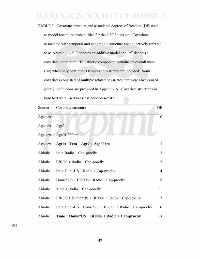
47

TABLE 3. Covariate structure and associated degrees of freedom (DF) used

to model recapture probabilities for the USGS data set. Covariates

associated with temporal and geographic structure are collectively referred

to as Abiotic. A “+” denotes an additive model and “*” denotes a

covariate interaction. The abiotic component contains an overall mean

(Int) when only continuous temporal covariates are included. Some

covariates consisted of multiple related covariates that were always used

jointly; definitions are provided in Appendix A. Covariate structures in

bold text were used to assess goodness-of-fit.

Source Covariate structure DF

Age-sex - 0

Age-sex Age2 1

Age-sex Age01.23Fem 1

Age-sex Age01.3Fem + Age2 + Age2Fem 3

Abiotic Int + Radio + Cap-procliv 3

Abiotic Eff-US + Radio + Cap-procliv 5

Abiotic Int + Hunt-US + Radio + Cap-procliv 4

Abiotic Home*US + BI2006 + Radio + Cap-procliv 5

Abiotic Time + Radio + Cap-procliv 11

Abiotic Eff-US + Home*US + BI2006 + Radio + Cap-procliv 7

Abiotic Int + Hunt-US + Home*US + BI2006 + Radio + Cap-procliv 6

Abiotic Time + Home*US + BI2006 + Radio + Cap-procliv 13

951

48

TABLE 4. Covariate structure and associated degrees of freedom (DF) used to model

recapture probabilities for the USCA data set. Covariates associated with temporal and

geographic structure are collectively referred to as Abiotic. A “+” denotes an additive

model and “*” denotes a covariate interaction. The abiotic component contains an overall

mean (Int) when only continuous temporal covariates are included. Some covariates

consisted of multiple related covariates that were always used jointly; definitions are

provided in Appendix A. Covariate structures in bold text were used to assess goodness-of-

fit.

Source Covariate structure DF

Age-sex UA 3

Age-sex Age2 + UA 4

Age-sex Age01.23Fem + UA 4

Age-sex Age01.3Fem + Age2 + Age2Fem + UA 6

Abiotic Int + Radio + Cap-procliv 3

Abiotic Int + Hunt + Radio + Cap-procliv 4

Abiotic Time + Radio + Cap-procliv 11

Abiotic Home + BI2006 + Eff-CA.1*CA + Radio + Cap-procliv 7

Abiotic Int + Hunt + Home + BI2006 + Eff-CA.l*CA + Radio + Cap-procliv 8

Abiotic Time + Home + BI2006 + Eff-CA.l*CA + Radio + Cap-procliv 15

Abiotic Eff-US*US + Eff-CA*CA + Radio + Cap-procliv 8

Abiotic Eff-US*US + Home*US + BI2006 + Eff-CA*CA + Radio + Cap-procliv 10

952

953

49

954

TABLE 5. The number of southern

Beaufort Sea polar bears captured (N),

and the number (M) and percentage

(%) that were previously marked, by

year in the USGS and USCA data sets.

USGS USCA

Year N M % N M %

2001 135 - - 135 - -

2002 118 36 30.5 118 36 30.5

2003 107 28 26.2 167 32 19.2

2004 148 39 26.4 291 64 22.0

2005 96 37 38.5 251 81 32.3

2006 90 40 44.4 150 64 42.7

2007 80 29 36.3 116 53 45.7

2008 88 35 39.8 108 49 45.4

2009 112 52 46.4 157 80 51.0

2010 75 38 50.7 97 45 46.4

955

956

50

TABLE 6. Total AICC model weight associated with covariate structures of

survival probability models, by age class, based on the USGS data set.

Covariate structures with a weight < 0.01 are excluded. A “+” denotes

an additive term and “*” denotes a covariate interaction. The adult

component contains an overall mean (Int) when only continuous

temporal covariates are included. Some covariates consisted of multiple

related covariates that were always used jointly; definitions are provided

in Appendix A.

Age class Covariate structure Weight

Cub Age0*TS-sur 0.781

Cub Age0 + Age0*Time-cubic 0.219

Yearling Age1 + Age1*Melt-season 0.424

Yearling Age1 + Age1*Time-cubic 0.245

Yearling Age1 + Age1*Summer-habitat 0.215

Yearling Age1*TS-sur 0.117

Subadult Age2 + Age2*Time-cubic + Age2Fem 0.536

Subadult Age2 + Age2*Melt-season + Age2Fem 0.402

Subadult Age2*TS-sur + Age2Fem 0.047

Subadult Age2 + Age2*Summer-habitat + Age2Fem 0.015

Adult Age3*TS-sur + Age3Fem 0.443

Adult Int + Age3*Time-cubic + Age3Fem 0.229

Adult Int + Age3*Melt-season + Age3Fem 0.210

Adult Int + Age3*Summer-habitat + Age3Fem 0.118

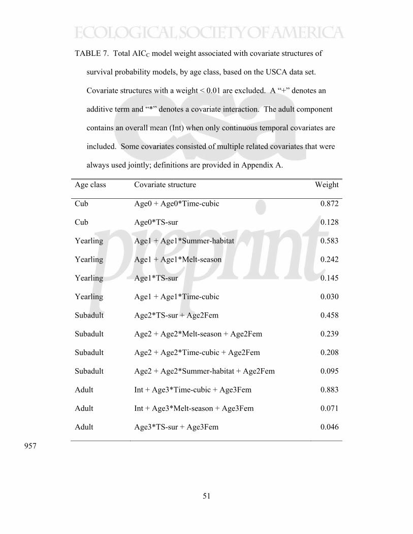
51

TABLE 7. Total AICC model weight associated with covariate structures of

survival probability models, by age class, based on the USCA data set.

Covariate structures with a weight < 0.01 are excluded. A “+” denotes an

additive term and “*” denotes a covariate interaction. The adult component

contains an overall mean (Int) when only continuous temporal covariates are

included. Some covariates consisted of multiple related covariates that were

always used jointly; definitions are provided in Appendix A.

Age class Covariate structure Weight

Cub Age0 + Age0*Time-cubic 0.872

Cub Age0*TS-sur 0.128

Yearling Age1 + Age1*Summer-habitat 0.583

Yearling Age1 + Age1*Melt-season 0.242

Yearling Age1*TS-sur 0.145

Yearling Age1 + Age1*Time-cubic 0.030

Subadult Age2*TS-sur + Age2Fem 0.458

Subadult Age2 + Age2*Melt-season + Age2Fem 0.239

Subadult Age2 + Age2*Time-cubic + Age2Fem 0.208

Subadult Age2 + Age2*Summer-habitat + Age2Fem 0.095

Adult Int + Age3*Time-cubic + Age3Fem 0.883

Adult Int + Age3*Melt-season + Age3Fem 0.071

Adult Age3*TS-sur + Age3Fem 0.046

957

52

Figure captions 958

FIG. 1. The upper panel contains a map of the Polar Basin, showing peripheral seas, 959

predominate currents, and ecoregions based upon characteristics of sea ice dynamics. The 960

lower panel shows the range of the southern Beaufort Sea polar bear population defined by 961

the International Union for Conservation of Nature, with a modified western boundary per 962

Amstrup et al. (2008), and locations of polar bear captures from 2001 to 2010 (yellow 963

circles). 964

FIG. 2. Anomalies (difference from the mean) of the two sea ice covariates from 1979 to 2010. 965

Normalized values from 2001 to 2010 (dark grey) were used to model polar bear survival 966

probabilities; (a) Summer-habitat, and (b) Melt-season. 967

FIG. 3. Model-averaged estimates of annual survival probability by age class and sex for the 968

USGS data set; (a) adult males, (b) adult females, (c) subadult males, (d) subadult females, 969

(e) yearlings, and (f) cubs. Error bars represent 90% bias-corrected bootstrap confidence 970

intervals based on 100 replications. 971

FIG. 4. Model-averaged estimates of annual survival probability by age class and sex for the 972

USCA data set; (a) adult males, (b) adult females, (c) subadult males, (d) subadult females, 973

(e) yearlings, and (f) cubs. Error bars represent 90% bias-corrected bootstrap confidence 974

intervals based on 100 replications. 975

FIG. 5. Model-averaged estimates of abundance based on (a) the USGS data set and (b) the 976

USCA data set. Error bars represent 90% bias-corrected confidence intervals based on 100 977

bootstrap samples. Prior estimates (Regehr et al. 2006) are shown for comparative purposes 978

(b, open diamonds). 979

980