1 riparian aquifer water budgets, climate and vegetation change t. meixner, j. hogan, j. stromberg,...

1

Riparian Aquifer Water Budgets, Riparian Aquifer Water Budgets, Climate and Vegetation ChangeClimate and Vegetation Change

T. Meixner, J. Hogan, J. Stromberg, K. Baird, T. Meixner, J. Hogan, J. Stromberg, K. Baird, M. Baillie, L. Klassner, P. Brooks, D. Goodrich, M. Baillie, L. Klassner, P. Brooks, D. Goodrich, H. Ajami, L. Vionnet, C. Vionnet, L. de la Cruz, H. Ajami, L. Vionnet, C. Vionnet, L. de la Cruz, A. McCoy, S. Simpson, C. Soto, S. TreeseA. McCoy, S. Simpson, C. Soto, S. Treese

University of Arizona – Hydrology and Water Resources, University of Arizona – Hydrology and Water Resources, SAHRA, Arid LandsSAHRA, Arid Lands

Arizona State University – Department of BiologyArizona State University – Department of Biology

USDA-ARS Southwest Watershed Research CenterUSDA-ARS Southwest Watershed Research Center

2

Where does water in the river come from?– Basin groundwater– Flood driven bank storage and riparian aquifer recharge– Human related sources – agricultural returns and WWTP

Are source and vegetation related? How important are floods?

– Annual and decadal scale variability could influence.– Seasonality of flooding – winter vs summer vs managed

What about this is important for management?– Floods are important– Mechanism not completely understood so specific plans of

action are not yet possible

OverviewOverview

3

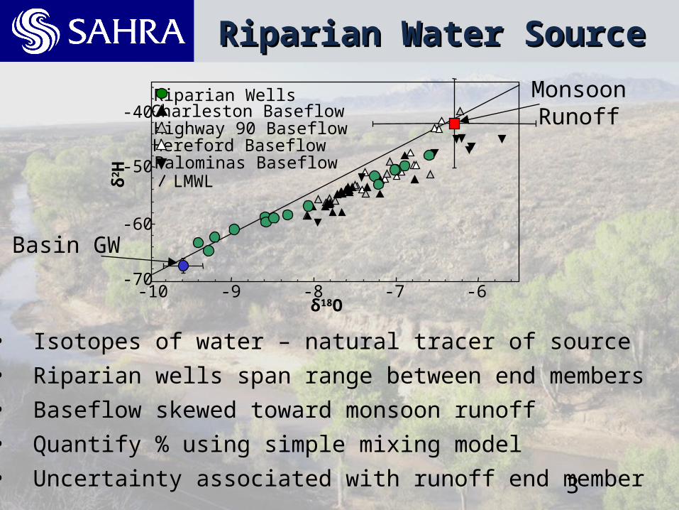
Riparian Water SourceRiparian Water Source

δ18O

-70

-60

-50

-40

-10 -9 -8 -7 -6

Riparian Wellsδ

2 HCharleston BaseflowHighway 90 BaseflowHereford BaseflowPalominas BaseflowLMWL

Basin GW

MonsoonRunoff

• Isotopes of water – natural tracer of source

• Riparian wells span range between end members

• Baseflow skewed toward monsoon runoff

• Quantify % using simple mixing model

• Uncertainty associated with runoff end member

4

Huachuca M

ountains

San Pedro River

Palominas

Hereford

Highway 90

Charleston

5 0 5Kilometers

N

Losing Reach

Legend:

Gaining Reach

Springs Surface WaterPrecipitationMountain Block

Wells

Mountain Front Wells

Basin Wells

Riparian Wells

Perennial Stream

Intermittent Stream

Losing/Gaining reach data from Stromberg et al. (in preparation); flow permanence data from the Nature Conservancy

Arizona

Sonora, Mexico

Study Area

New

Mexico

Nev

ada

Cal

ifor

nia

Utah

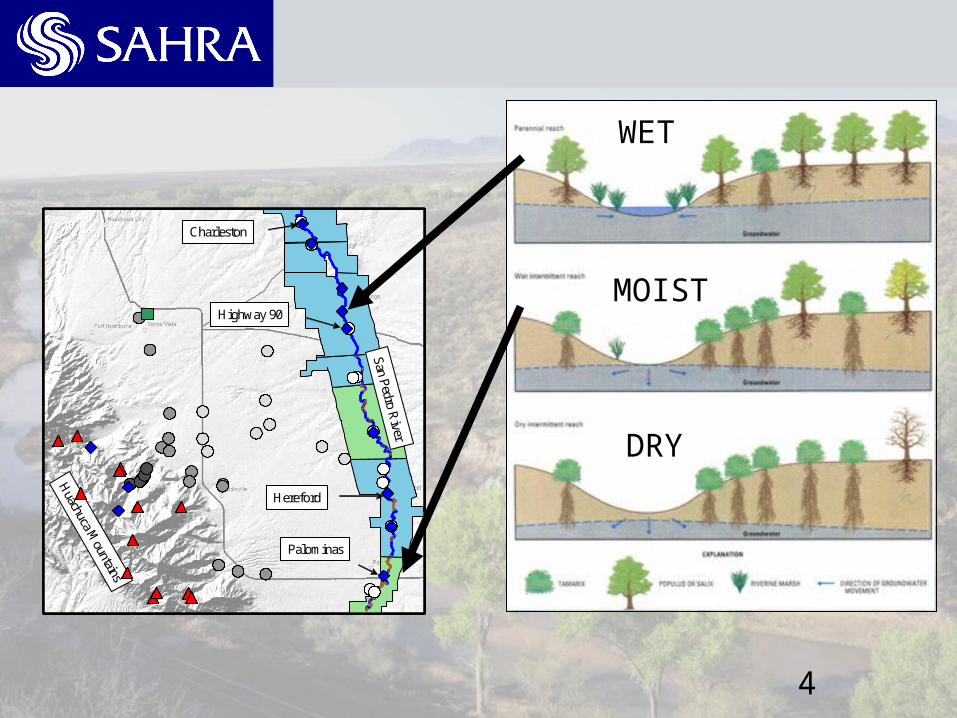
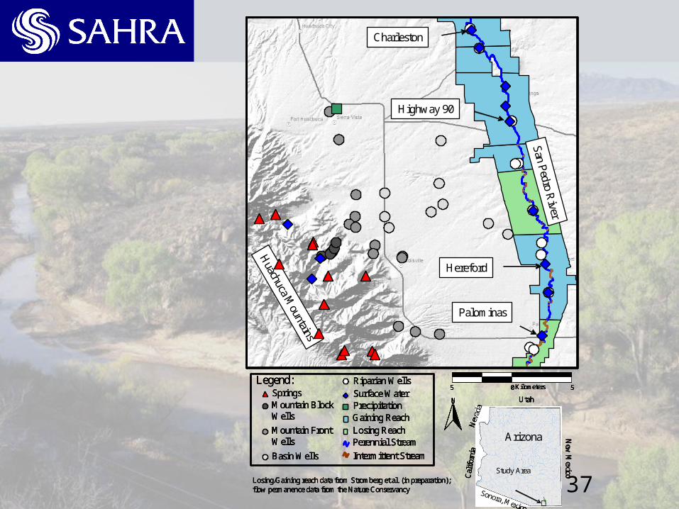
Figure 1: Map of the study area. Sampling locations are noted by symbols. The river is divided into wet and dry reaches using data collected by the Nature Conservancy in June of 2003. Additionally, information on condition classes, dividing the riparian area into gaining and losing reaches (Stromberg et al., in press), is included along the river. Blue areas are gaining, and green areas are losing; the outline of the reaches corresponds to the extent of the San Pedro River National Conservation Area. Note the presence of the Palominas surface water sampling site in a losing reach, whereas the Hereford, Highway 90, and Charleston sampling sites are located in gaining reaches.

Huachuca M

ountains

San Pedro River

Palominas

Hereford

Highway 90

Charleston

5 0 5Kilometers

N

Losing Reach

Legend:

Gaining Reach


Wells


Basin Wells

Riparian Wells

Perennial Stream

Intermittent Stream


Arizona

Sonora, Mexico

Study Area

New

Mexico

Nev

ada

Cal

ifor

nia

Utah

Huachuca M

ountains

San Pedro River

Palominas

Hereford

Highway 90

Charleston

5 0 5Kilometers5 0 5Kilometers

NN

Losing Reach

Legend:

Gaining Reach


Wells


Basin Wells

Riparian Wells

Perennial Stream

Intermittent Stream


Arizona

Sonora, Mexico

Study Area

New

Mexico

Nev

ada

Cal

ifor

nia

Utah


WET

MOIST

DRY

5

2.2

2.7

2.7

2.6

6

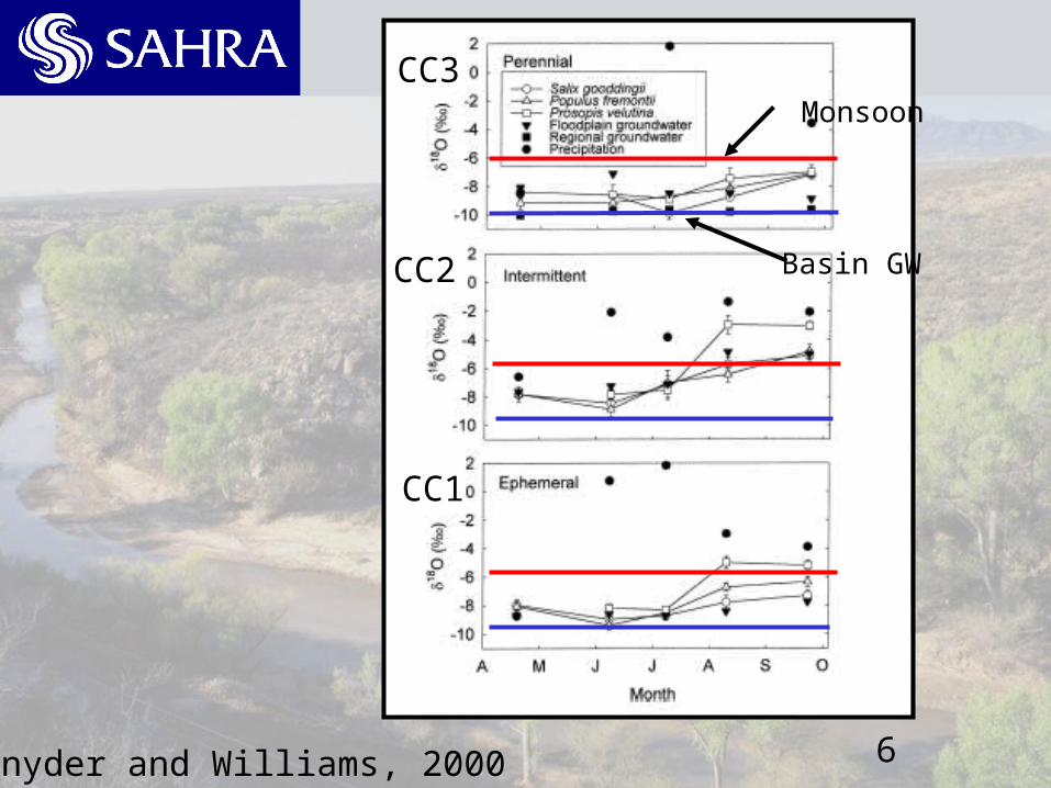
Monsoon

Basin GW

Snyder and Williams, 2000

CC3

CC2

CC1

7

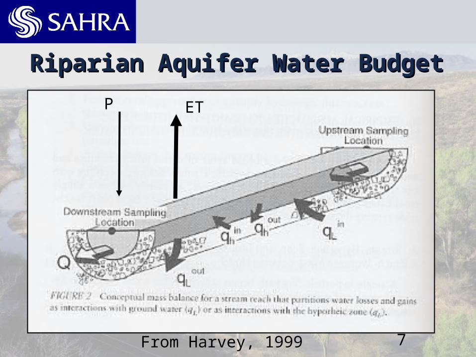
Riparian Aquifer Water BudgetRiparian Aquifer Water Budget

ETP

From Harvey, 1999

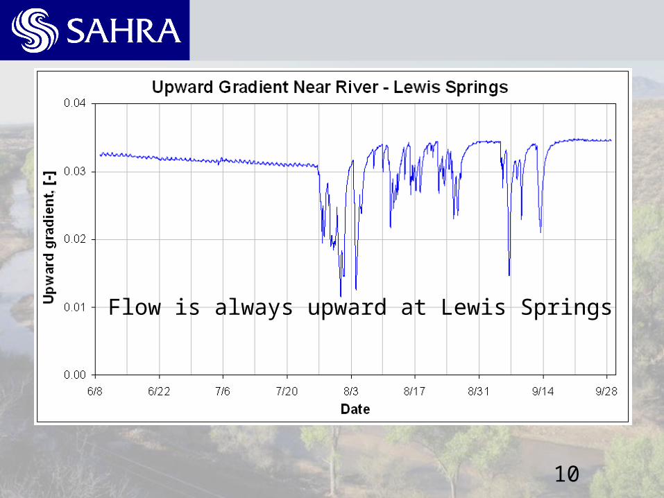
10

Flow is always upward at Lewis Springs

11

Flow Towards River

Flow Away From River

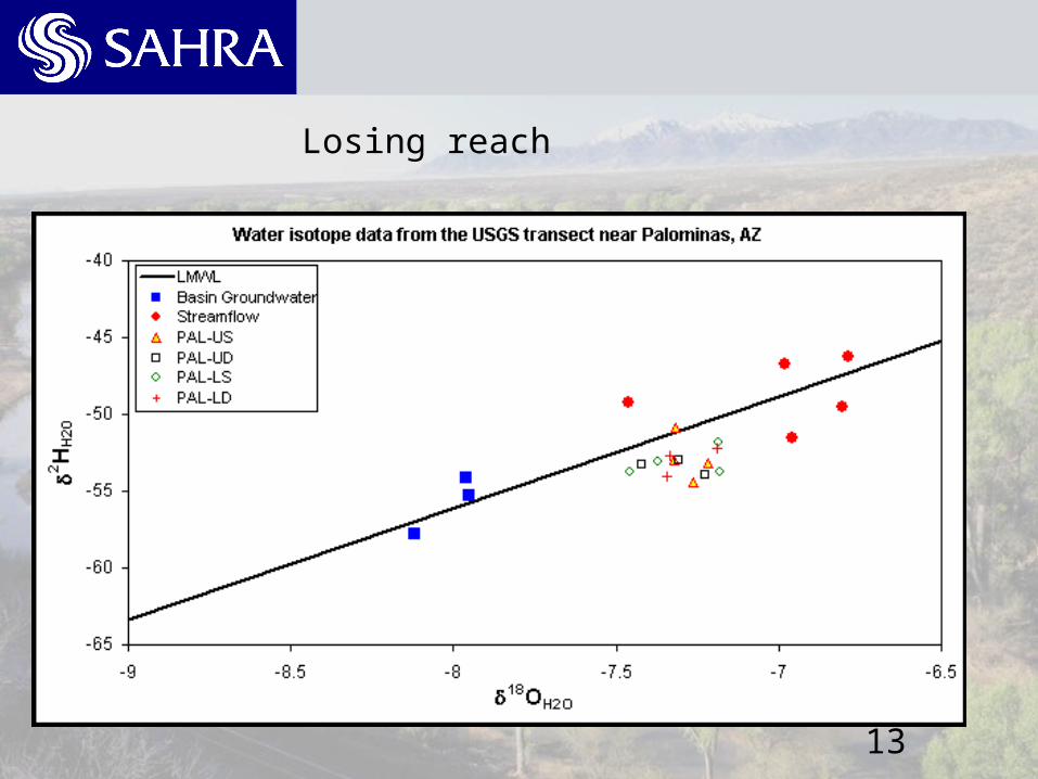
13

Losing reach

15

Gaining vs LosingGaining vs LosingBasin Groundwater in Riparian Wells

Groundwater inflow from south?

Depth of Well (ft)

Perc

en

t B

asin

Gro

un

dw

ate

r

0%

20%

40%

60%

80%

100%

0 50 100 150 200

Gaining Reach Losing Reach

16

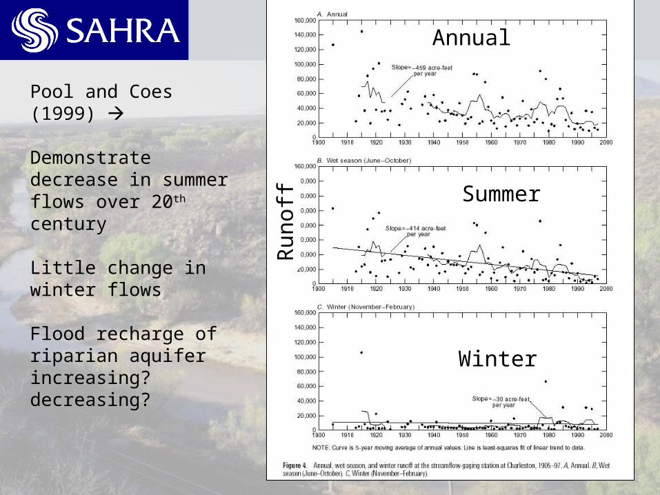
Pool and Coes (1999)

Demonstrate decrease in summer flows over 20th century

Little change in winter flows

Flood recharge of riparian aquifer increasing? decreasing?

Annual

Summer

Winter

Run

off

18

Importance of Alluvial Aquifers in Semi-Arid Systems

– Riparian ecosystems (Stromberg et al)– Physical integrators (Hogan)– Provide water for human and ecological systems

Take home message– We know flood recharge is an important water source in

the San Pedro.– We know it is affected by climate related flood variability – But we do not understand the mechanism and the

dynamic link to climate.

20

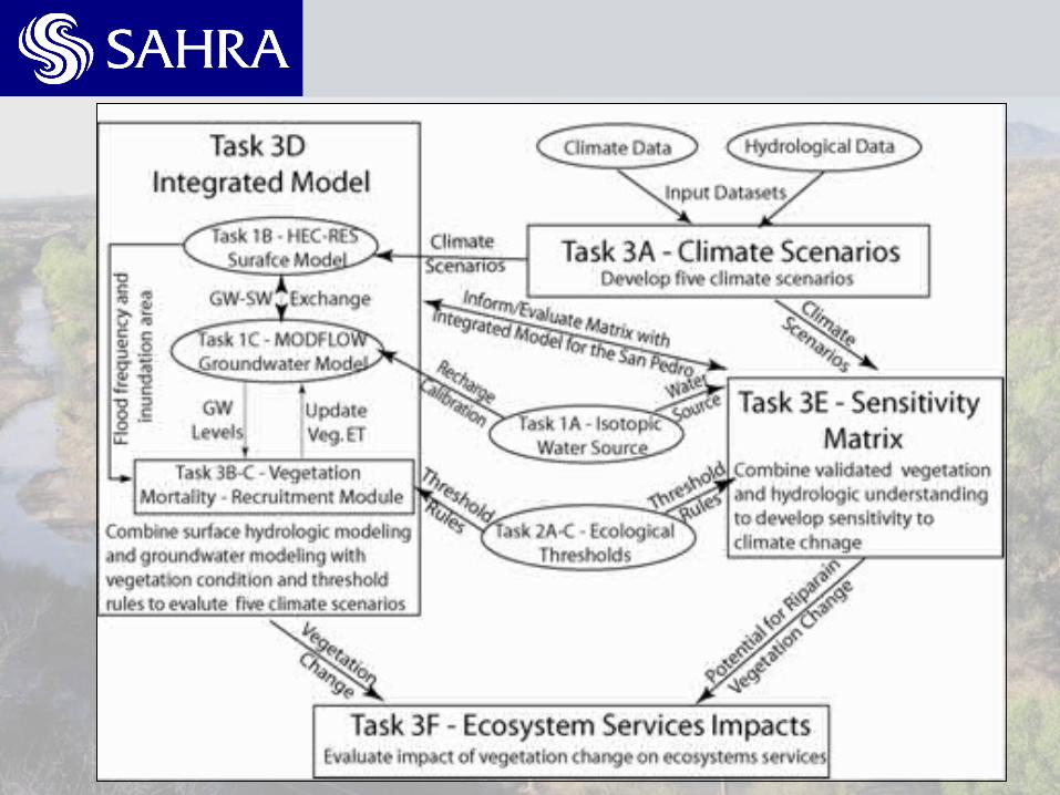
SWAT - Nutrient Flood FlowsKINEROS – Sediment Flood Flows

Flood Flows

Basin Groundwater

Nutrient Rich Downstream Flood Waters

In River/Riparian ET/ Nutrient Processing MODFLOW/KINEROS/CENTURY/HYDRUS

23

Decadal Scale Climate VariabilityDecadal Scale Climate VariabilityRiparian Vegetation Change Riparian Vegetation Change EPA STAREPA STAR

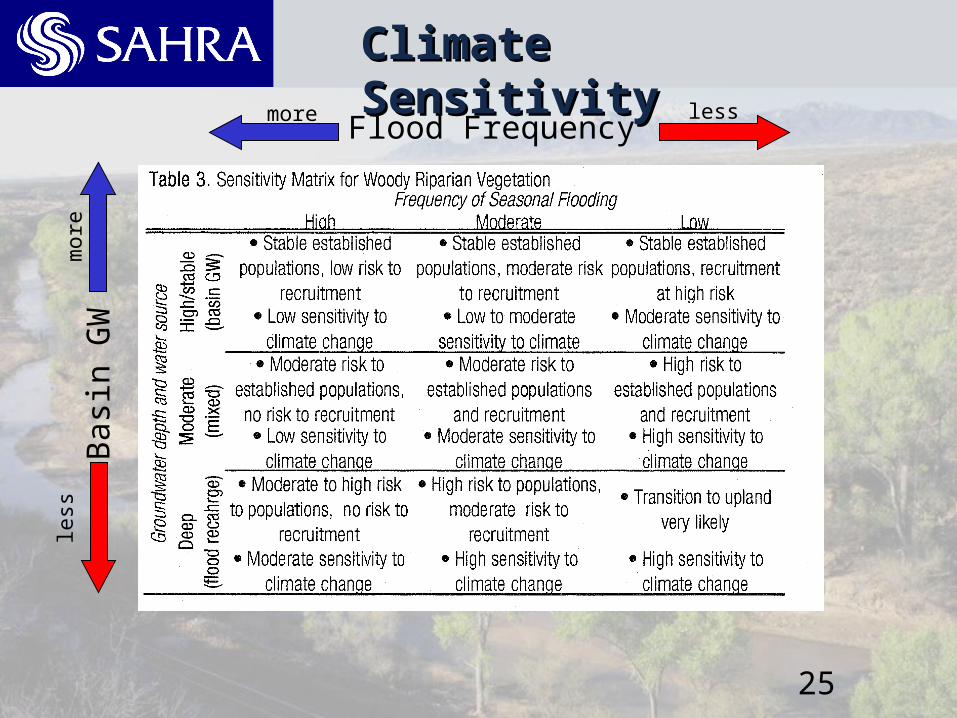
1) Riparian aquifer recharge depends on flood characteristics and dominates in reaches with minimal regional aquifer connection.

2) Riparian vegetation structure responds non-linearly as riparian aquifers are dewatered and thresholds for survivorship are exceeded.

3) Decadal scale climate variability alters riparian ecosystem water budgets and ecosystem structure and function.

24

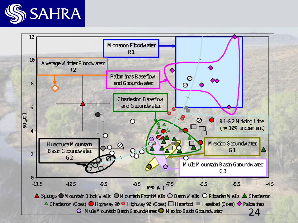
Mexico GroundwaterG1

0

2

4

6

8

10

12

-11.5 -10.5 -9.5 -8.5 -7.5 -6.5 -5.5 -4.5

Mountain Block Wells Mountain Front Wells Basin Wells Riparian WellsSprings

PalominasHerefordHighway 90

Charleston

SO

4/C

l

δ18O (‰)

Huachuca Mountain Basin Groundwater

G2

Palominas Baseflowand Groundwater

Monsoon FloodwaterR1

Hereford (Coes)Highway 90 (Coes)Charleston (Coes)

Charleston Baseflowand Groundwater

Average Winter FloodwaterR2

Mexico Basin GroundwaterMule Mountain Basin Groundwater

Mule Mountain Basin GroundwaterG3

R1-G2 Mixing Line( = 10% increment)


0

2

4

6

8

10

12

-11.5 -10.5 -9.5 -8.5 -7.5 -6.5 -5.5 -4.5



Charleston

SO

4/C

l

δ18O (‰)


G2









25

Climate SensitivityClimate Sensitivity

Flood FrequencyB

asin

GW

less

less

mor

e

more

26

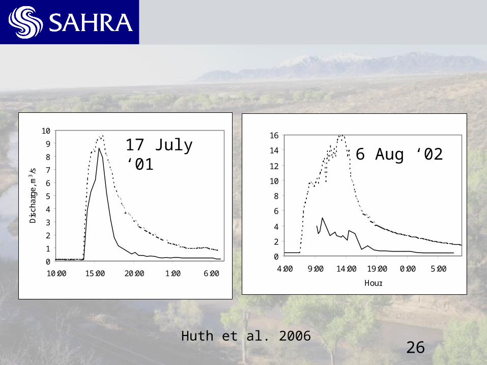
0

1

2

3

4

5

6

7

8

9

10

10:00 15:00 20:00 1:00 6:00

Dis

char

ge, m

3/s

17 July ‘01

0

2

4

6

8

10

12

14

16

4:00 9:00 14:00 19:00 0:00 5:00

Hour

6 Aug ‘02

Huth et al. 2006

27

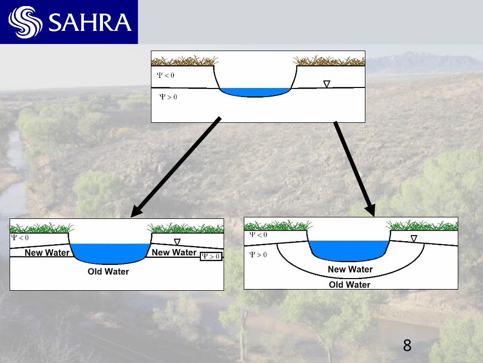
Alluvial Aquifer Monsoon RechargeAlluvial Aquifer Monsoon Recharge Is this water “new”? This effects current sustainable flow calculations

– Traditional assumption is basin groundwater budget need not account for floods

– Assumption needs to be reassessed Monsoon flood recharge may not be “additional water”

– Old water versus new water debate– Mechanism may be similar here– Flood waters observed may have simply displaced existing

water– Flood wave water may have been added to the “top” of the

aquifer What fraction of flood waters are basin groundwater? How much of monsoon water presence in alluvial aquifer

displaces existing groundwater versus adds new water to alluvial aquifer?

28

Alluvial AquifersAlluvial Aquifers Science

– Semi-arid systems ideal to study alluvial aquifers– Isolation from hillslope processes– Mechanism of interaction, storage and release

Interesting interaction between storm behavior (Huth et al. 2006)

And seasonal to inter-annual behavior (Baillie and Hogan 2006)

Broader Impacts– Critical for

Sustaining streamflow Sustaining vegetation

– Susceptible to Human Impacts Changes in Flood Patterns Changes in Climate

29

0

2

4

6

8

10

12

14

0 1 2 3 4 5 6

ET (mm/day)

dept

h (m

)

Mesquite

Cottonw ood

Tamarisk

Sacaton

Evap0

2

4

6

8

10

12

14

0 1 2 3 4 5 6

ET (mm/day)

dept

h (m

)

Mesquite

Cottonw ood

Tamarisk

Sacaton

0

2

4

6

8

10

12

14

0 1 2 3 4 5 6

ET (mm/day)

dept

h (m

)

Mesquite

Cottonw ood

Tamarisk

Sacaton

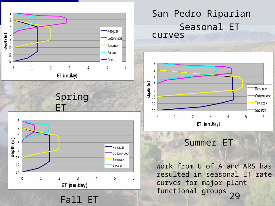
San Pedro Riparian

Seasonal ET curves

Spring ET

Summer ET

Fall ET

Work from U of A and ARS has resulted in seasonal ET rate curves for major plant functional groups

30

SWAT - Nutrient Flood FlowsKINEROS – Sediment Flood Flows

Flood Flows

Basin Groundwater

Nutrient Rich Downstream Flood Waters

In River/Riparian ET/ Nutrient Processing MODFLOW/KINEROS/CENTURY/HYDRUS

31

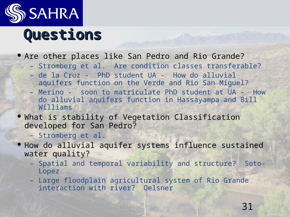
QuestionsQuestions Are other places like San Pedro and Rio Grande?

– Stromberg et al. Are condition classes transferable?– de la Cruz - PhD student UA - How do alluvial aquifers function

on the Verde and Rio San Miguel?– Merino - soon to matriculate PhD student at UA - How do

alluvial aquifers function in Hassayampa and Bill Williams What is stability of Vegetation Classification developed for

San Pedro?– Stromberg et al.

How do alluvial aquifer systems influence sustained water quality?

– Spatial and temporal variability and structure? Soto-Lopez– Large floodplain agricultural system of Rio Grande interaction

with river? Oelsner

32

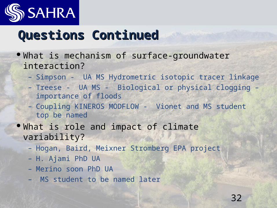
Questions ContinuedQuestions Continued What is mechanism of surface-groundwater

interaction?– Simpson - UA MS Hydrometric isotopic tracer linkage– Treese - UA MS - Biological or physical clogging –

importance of floods– Coupling KINEROS MODFLOW - Vionet and MS student

top be named What is role and impact of climate variability?

– Hogan, Baird, Meixner Stromberg EPA project– H. Ajami PhD UA– Merino soon PhD UA– MS student to be named later

33

2.0

2.5

3.0

3.5

4.0

4.5

5.0

0 1000 2000 3000 4000 5000 6000 7000 8000 9000 10000

Distance (m)

March May

River Flow

Sulfate/Chloride Ratio near San Pedro House

34

San Pedro Changes in RunoffSan Pedro Changes in Runoff

Pool and Coes, 1999

•Decline in runoff•No change in PPT•Change in intensity?•Vegetation change?

•Decline in baseflow•Change in flood recharge?

35

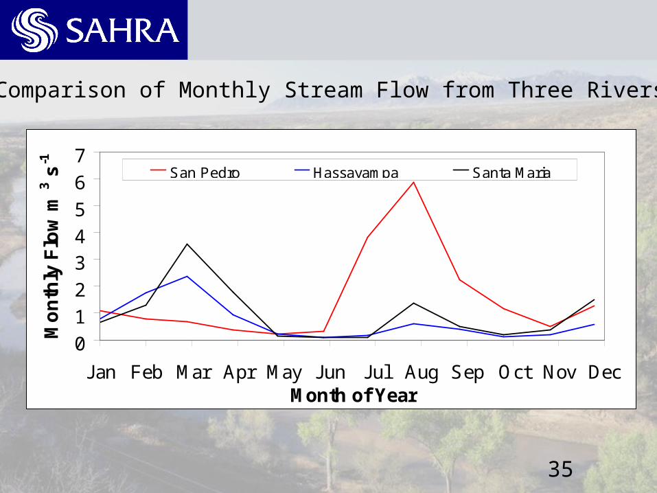
0

1

2

34

5

6

7

Jan Feb Mar Apr May Jun Jul Aug Sep Oct Nov DecMonth of Year

Mo

nth

ly F

low

m3 s

-1

San Pedro Hassayampa Santa Maria

Comparison of Monthly Stream Flow from Three Rivers

36

-12 -11 -10 -9 -8 -7 -6-80

-75

-70

-65

-60

-55

-50

-45

-40

δ18O (‰)

δ2H

(‰)

Legend:SpringsMountain Block WellsMountain Front WellsBasin WellsRiparian WellsAvg. Summer PrecipAvg. Winter PrecipMixing LineWinter PrecipContribution

Basin Groundwater

Riparian Groundwater

100%

75%

50%

25%

0%

75%

Figure 3: Stable isotopic composition of groundwater. Values for springs, mountain block wells, and mountain front wells are represented as the average value ±1σ and are discussed in detail in Wahi et al. (in preparation). Summer precipitation average is for April 15 through October 15, and winter average is for October 15 through April 15.

-12 -11 -10 -9 -8 -7 -6-80

-75

-70

-65

-60

-55

-50

-45

-40

δ18O (‰)

δ2H

(‰)


Basin Groundwater


100%

75%

50%

25%

0%

75%

-12 -11 -10 -9 -8 -7 -6-80

-75

-70

-65

-60

-55

-50

-45

-40

δ18O (‰)

δ2H

(‰)


Basin Groundwater

Basin Groundwater



100%

75%

50%

25%

0%

75%

Figure 3: Stable isotopic composition of groundwater. Values for springs, mountain block wells, and mountain front wells are represented as the average value ±1σ and are discussed in detail in Wahi et al. (in preparation). Summer precipitation average is for April 15 through October 15, and winter average is for October 15 through April 15.

SUMMER

WINTER

37

Huachuca M

ountains

San Pedro River

Palominas

Hereford

Highway 90

Charleston

5 0 5Kilometers

N

Losing Reach

Legend:

Gaining Reach


Wells


Basin Wells

Riparian Wells

Perennial Stream

Intermittent Stream


Arizona

Sonora, Mexico

Study Area

New

Mexico

Nev

ada

Cal

ifor

nia

Utah


Huachuca M

ountains

San Pedro River

Palominas

Hereford

Highway 90

Charleston

5 0 5Kilometers

N

Losing Reach

Legend:

Gaining Reach


Wells


Basin Wells

Riparian Wells

Perennial Stream

Intermittent Stream


Arizona

Sonora, Mexico

Study Area

New

Mexico

Nev

ada

Cal

ifor

nia

Utah

Huachuca M

ountains

San Pedro River

Palominas

Hereford

Highway 90

Charleston

5 0 5Kilometers5 0 5Kilometers

NN

Losing Reach

Legend:

Gaining Reach


Wells


Basin Wells

Riparian Wells

Perennial Stream

Intermittent Stream


Arizona

Sonora, Mexico

Study Area

New

Mexico

Nev

ada

Cal

ifor

nia

Utah


38


0

2

4

6

8

10

12

-11.5 -10.5 -9.5 -8.5 -7.5 -6.5 -5.5 -4.5



Charleston

SO

4/C

l

δ18O (‰)


G2










0

2

4

6

8

10

12

-11.5 -10.5 -9.5 -8.5 -7.5 -6.5 -5.5 -4.5



Charleston

SO

4/C

l

δ18O (‰)


G2









1 riparian aquifer water budgets, climate and vegetation change t. meixner, j. hogan, j. stromberg,...

Documents

river slide

riparian water source

reachlosing reach slide

possible overview slide

lewis springs slide

riparian aquifers

riparian aquifer water

runoff end member slide