1. report date 2. report type journal article · report documentation page ... correlation of rp-1...

REPORT DOCUMENTATION PAGE Form Approved

OMB No. 0704-0188 Public reporting burden for this collection of information is estimated to average 1 hour per response, including the time for reviewing instructions, searching existing data sources, gathering and maintaining the data needed, and completing and reviewing this collection of information. Send comments regarding this burden estimate or any other aspect of this collection of information, including suggestions for reducing this burden to Department of Defense, Washington Headquarters Services, Directorate for Information Operations and Reports (0704-0188), 1215 Jefferson Davis Highway, Suite 1204, Arlington, VA 22202-4302. Respondents should be aware that notwithstanding any other provision of law, no person shall be subject to any penalty for failing to comply with a collection of information if it does not display a currently valid OMB control number. PLEASE DO NOT RETURN YOUR FORM TO THE ABOVE ADDRESS.

1. REPORT DATE (DD-MM-YYYY) September 2013

2. REPORT TYPEJournal Article

3. DATES COVERED (From - To) September 2013- February 2014

4. TITLE AND SUBTITLE Correlation of RP-1 Fuel Properties with Chemical Composition using Two-Dimensional Gas Chromatography with Time-of-Flight Mass Spectrometry followed by Partial Least Squares Regression Analysis

5a. CONTRACT NUMBER In-House

5b. GRANT NUMBER 5c. PROGRAM ELEMENT NUMBER

6. AUTHOR(S) Kehimkar, B., J. Hoggard, L. Marney, M. Billingsley, C. Fraga, T. Bruno, and R. Synovec

5d. PROJECT NUMBER

5e. TASK NUMBER 5f. WORK UNIT NUMBER

Q0A4 7. PERFORMING ORGANIZATION NAME(S) AND ADDRESS(ES) 8. PERFORMING ORGANIZATION

REPORT NO.Air Force Research Laboratory (AFMC) AFRL/RQRC 10 E. Saturn Blvd. Edwards AFB CA 93524-7680

9. SPONSORING / MONITORING AGENCY NAME(S) AND ADDRESS(ES) 10. SPONSOR/MONITOR’S ACRONYM(S)Air Force Research Laboratory (AFMC) AFRL/RQR 5 Pollux Drive 11. SPONSOR/MONITOR’S REPORT

Edwards AFB CA 93524-7048 NUMBER(S)

AFRL-RQ-ED-JA-2013-227

12. DISTRIBUTION / AVAILABILITY STATEMENT Distribution A: Approved for Public Release; Distribution Unlimited. PA#13513

13. SUPPLEMENTARY NOTES Journal Article submitted to Journal of Chromatography A.

14. ABSTRACT There is an increased need to more fully assess and control the composition of kerosene-based rocket propulsion fuels such as RP-1. In particular, it is critical to make better quantitative connections among the following three attributes: fuel performance (thermal stability, sooting propensity, engine specific impulse, etc.), fuel properties (such as flash point, density, kinematic viscosity, net heat of combustion, hydrogen content, etc.), and the chemical composition of a given fuel, i.e., amounts of specific chemical compounds and chemical groups present in a fuel as a result of feedstock blending and/or processing. Recent efforts in predicting fuel chemical and physical behavior through modeling put greater emphasis on attaining detailed and accurate fuel properties and fuel composition information. Often, one-dimensional gas chromatography (GC) combined with mass spectrometry (MS) is employed to provide chemical composition information. Building on approaches that make use of GC-MS, but to glean substantially more chemical composition information from these complex fuels, we have recently studied the use of comprehensive two dimensional (2D) gas chromatography combined with time-of-flight mass spectrometry (GC × GC – TOFMS) using a “reversed column” format: RTX-wax column for the first dimension, and a RTX-1 column for the second dimension. In this report, by applying chemometric data analysis, specifically partial least-squares (PLS) regression analysis, we are able to readily model (and correlate) the chemical compositional information provided by use of GC × GC – TOFMS to RP-1 fuel property information such as density, kinematic viscosity, net heat of combustion, hydrogen content, and so on. Furthermore, we readily identified compounds that contribute significantly to measured differences in fuel properties based on results from the PLS models. We anticipate this new chemical analysis strategy will have broad implications for the development of high fidelity composition-property models, leading to an improved approach to fuel formulation and specification for advanced engine cycles.

15. SUBJECT TERMS

16. SECURITY CLASSIFICATION OF:

17. LIMITATION OF ABSTRACT

18. NUMBER OF PAGES

19a. NAME OF RESPONSIBLE PERSON

Matt Billingsley

a. REPORT Unclassified

b. ABSTRACT Unclassified

c. THIS PAGE Unclassified

SAR 72 19b. TELEPHONE NO (include area code)

661-525-5885 Standard Form

298 (Rev. 8-98) Prescribed by ANSI Std. 239.18

Correlation of RP-1 fuel properties with chemical composition

using comprehensive two-dimensional gas chromatography with time-of-flight mass spectrometry

followed by partial least squares regression analysis

Benjamin Kehimkara, Jamin C. Hoggard

a, Luke C. Marney

a, Matthew C. Billingsley

b,

Carlos G. Fragac, Thomas J. Bruno

d and Robert E. Synovec

a,*

a Department of Chemistry, Box 351700, University of Washington

Seattle, WA 98195, USA

b Air Force Research Laboratory/RQRC, 10 E Saturn Blvd.

Edwards AFB, CA 93524, USA

c Pacific Northwest National Laboratory, PO Box 999 MS P7-50

Richland, WA 99352, USA

d Applied Chemicals and Materials Division, National Institute of Standards and Technology

Boulder, CO 80305, USA

* Corresponding author at: Department of Chemistry, University of Washington, Seattle, WA

98195-1700, USA. Tel.:+1 206 685 2328; fax: +1 206 685 8665.

E-mail address: [email protected] (R. E. Synovec).

Prepared for submission to Journal of Chromatography A

September 4, 2013

mailto:[email protected]

1071010496E

Typewritten Text

1071010496E

Typewritten Text

Distribution A: Approved for Public Release; Distribution Unlimited

1071010496E

Typewritten Text

1071010496E

Typewritten Text

1071010496E

Typewritten Text

1071010496E

Typewritten Text

2

Abstract

There is an increased need to more fully assess and control the composition of kerosene-based

rocket propulsion fuels such as RP-1. In particular, it is critical to make better quantitative connections

among the following three attributes: fuel performance (thermal stability, sooting propensity, engine

specific impulse, etc.), fuel properties (such as flash point, density, kinematic viscosity, net heat of

combustion, hydrogen content, etc.), and the chemical composition of a given fuel, i.e., amounts of

specific chemical compounds and chemical groups present in a fuel as a result of feedstock blending

and/or processing. Recent efforts in predicting fuel chemical and physical behavior through modeling

put greater emphasis on attaining detailed and accurate fuel properties and fuel composition information.

Often, one-dimensional gas chromatography (GC) combined with mass spectrometry (MS) is employed

to provide chemical composition information. Building on approaches that make use of GC-MS, but to

glean substantially more chemical composition information from these complex fuels, we have recently

studied the use of comprehensive two dimensional (2D) gas chromatography combined with time-of-

flight mass spectrometry (GC × GC – TOFMS) using a “reversed column” format: RTX-wax column for

the first dimension, and a RTX-1 column for the second dimension. In this report, by applying

chemometric data analysis, specifically partial least-squares (PLS) regression analysis, we are able to

readily model (and correlate) the chemical compositional information provided by use of GC × GC –

TOFMS to RP-1 fuel property information such as density, kinematic viscosity, net heat of combustion,

hydrogen content, and so on. Furthermore, we readily identified compounds that contribute significantly

to measured differences in fuel properties based on results from the PLS models. We anticipate this new

chemical analysis strategy will have broad implications for the development of high fidelity

composition-property models, leading to an improved approach to fuel formulation and specification for

advanced engine cycles.

KEYWORDS: GC × GC – TOFMS, PLS, Chemometrics, Gas Chromatography, RP-1, Kerosene.

3

1. Introduction

The chemical composition of a kerosene fuel is complex, and changes in composition have been

widely demonstrated to impact fuel properties and performance [1-4]. However, achieving precise

control over the chemical composition of distillate fuels such as RP-1 (MIL-DTL-25576E) is

challenging due to variations in crude oil composition and place of origin, refinery and post-refinery

operating conditions, or even the date and time the material was refined, treated, and formulated to meet

the detail specification requirements. A better understanding of fuel composition and how it relates to

fuel performance and properties is expedient for a number of reasons. Indeed, it has become

increasingly important to gain a better understanding of fuel composition, and an assessment of the

potential sources of fuel composition variation is paramount to maintain control of fuel performance

[5-11]. It is also beneficial to relate new chemical analysis technologies to the benchmarking ASTM

methods for characterizing properties and compositions of fuels such as RP-1. For such assessments, it

is often beneficial to evaluate special laboratory blends (where the analyst has some control over the

chemical composition, see Table 1) as well as to assess the performance of “field” fuels [5-9].

Gas chromatography coupled with mass spectrometry (GC-MS) is an established workhorse tool

of the chemical analysis laboratory. GC is ideally suited to the separation of complex samples such as

multi-component hydrocarbon fuels [7, 8, 12, 13], because GC has the ability to spatially separate a

large number of chemical compounds. Adding MS for detection provides a substantial increase in the

chemical selectivity of this instrumental platform. GC-MS has proven itself as a powerful tool for the

study of the chemical composition of fuels [5, 6, 9, 10, 12, 14]. Nevertheless, GC-MS can be made

substantially more powerful by adding another dimension of separation, that is, by performing

comprehensive two-dimensional (2D) gas chromatography prior to time-of-flight mass spectrometry

detection (GC × GC – TOFMS) [15-23]. The added dimension of separation provides a substantial

4

improvement in chemical selectivity relative to GC-MS. Although the TOFMS provides unit mass

resolution, GC × GC allows for detailed analyses with reasonable file sizes and manageable data

analyses. GC × GC – TOFMS is well suited for the analysis of complex mixtures of volatile (and/or

semi-volatile) compounds, such as are present in fuels [15-17, 19-24]. The GC × GC – TOFMS

instrument produces data consisting of a complete mass spectrum collected at each detection sampling

point of a 2D separation. The 2D separation provides temporal separation for each analyte compound

peak from the peaks of most of the other compounds in the mixture, while imposing a patterned

structure formed by the retention times at which peaks for different related compounds appear, which

depends on the separation conditions.

With GC × GC – TOFMS, a 2D separation is commonly produced with the first separation

dimension performed using a non-polar stationary phase column and a separation run time of 30 to 60

minutes [15, 16, 24]. In the second dimension, a polar stationary phase column is commonly used,

providing a complementary separation relative to the first column, so chemical compounds not separated

on the first dimension at a given retention time have the opportunity to be separated on the second

dimension. However, for the study of RP-1 fuels, which contain primarily n-alkanes, iso-alkanes, cyclic

alkanes, and aromatics, it was deemed necessary to apply a “reversed column” GC × GC format in order

to provide good selectivity [25], with the first dimension separation using a polar phase (RTX-wax) and

the second dimension separation using a non-polar phase (RTX-1). The TOFMS detects analyte

compounds as they leave the second column. Each analyte produces a chromatographic peak in the

second dimension with a width on the order of ~ 100 ms. The mass spectral acquisition rate for the

TOFMS used for this report is 500 Hz with an m/z range of 5 - 1000, yielding ~ 50 spectra per second

dimension peak. For most GC-based fuel studies, however, an m/z range of 40 – 400 m/z is sufficient.

Thus, GC × GC – TOFMS provides a considerable amount of data for a given complex sample (e.g.,

5

typically ~ 300 to 400 MB compressed per sample run). It has become clear that there are also

significant challenges to readily gleaning useful information from this significant amount of data, which

is why powerful chemometric software methods are used for analysis [15-24, 26-28].

Even though GC × GC – TOFMS is a powerful instrumental platform for fuels analysis, it is

critical to develop and apply data analysis software that can readily convert the immense data into

readily interpretable and useful information. For this purpose, multivariate data analysis methods have

been developed, broadly referred to as “chemometrics”. Chemometric data analysis is ideally suited for

analyzing and to reveal similarities and/or differences between sets of GC × GC – TOFMS data [15-17,

20-22, 28]. Specific to this study, the chemometric method partial least-squares (PLS) regression

analysis was used to associate differences in measurable information for each fuel sample, in this case

chemical and physical property data, to chemical composition differences in a corresponding set of fuel

samples. Details on the theory of PLS can be found elsewhere [29-31]. Briefly, PLS analyzes two data

matrices (X-block and Y-block, respectively) and calculates orthogonal components similar to principal

components (PCs) in principal component analysis (PCA), except that the PCs in the X-block have a

maximum covariance with their respective PCs in the Y-block. In other words, PC1 in the X-block

would have maximum covariance with PC1 of Y-block, and so on. To make the distinction, the “PCs”

in PLS are commonly known as Latent Variables (LVs). Using PLS, models can be constructed to

account for variance (ideally, the relevant chemical differences) in both the GC × GC – TOFMS data

(which constitute the X-block) and the respective measured property values (which constitute the Y-

block). These variances are also correlated to determine what differences in the GC × GC – TOFMS

data account for differences in the measured property values. It is important to examine how well the

predicted values provided by the PLS model match the measured value properties, as this is a good

indication of the quality of the model (i.e., if variance has been captured that accounts for the change in

6

the measured variables). Moreover, validating the models is also important. Herein, validation was

performed using a second set of replicates to test the predictive ability of the model.

In this study, we sought to demonstrate the potential of the GC × GC – TOFMS instrumental

platform, combined with chemometric data analysis, to provide useful information in the chemical

analysis of RP-1 samples. By doing so, our goals were to demonstrate the feasibility of being able to (1)

build PLS models that relate chemical composition data obtained from the GC × GC – TOFMS to

measured fuel performance quantities (e.g., density, kinematic viscosity, net heat of combustion,

hydrogen content, and so on), and then to (2) use those models for subsequent prediction of fuel

chemical and physical characteristics without making direct measurements. Eventually, this chemical

analysis approach will provide insight into addressing (3) the overall goal of optimizing fuel

composition to meet desired fuel property and performance characteristics. To begin to address these

goals by use of GC × GC – TOFMS with chemometric data analysis, a key focus is to be able to

elucidate chemical compounds or classes of compounds responsible for observed differences between

fuels (e.g. type, feedstock) or differences in their measured physical properties. Specifically we report

the use of GC × GC – TOFMS with PLS to model and predict measured fuel properties (density,

hydrogen content, kinematic viscosity, net heat of combustion) [6].

2. Experimental

Several RP-1 fuel samples were obtained from the Air Force Research Laboratory (AFRL), most

of which have been studied in prior reports [5, 6]. The list of RP-1 fuels used can be found in Table 1.

All chromatographic data was obtained using the GC × GC – TOFMS consisting of an Agilent 6890N

GC (Agilent Technologies, Palo Alto, CA, USA), a thermal modulator (4D upgrade, LECO, St. Joseph,

MI, USA), and a Pegasus III TOFMS (LECO, St. Joseph, MI, USA). Aliquots of RP-1 fuel samples

were introduced to the GC × GC – TOFMS instrument via a 7683B auto-injector (Agilent Technologies,

7

Palo Alto, CA, USA). The following experimental conditions were applied. The auto-injector was set

to a 1 μl injection, using a 200:1 split injection with helium carrier gas. Acetone was used for the

solvent rinse. Isobaric mode was used with an inlet pressure of 35 psig (241 kPa). The GC oven initial

temperature was set to 40 °C for 2 min and ramped to 225 °C at a rate of 6 °C/min where the final

temperature was maintained for 3 min. The GC inlet temperature was set to 225 °C and the transfer line

temperature was set to 235 °C. The thermal modulator offset was 20 °C, with a hot pulse time of 0.59 s

and a cool time of 0.35 s. The primary column (first separation dimension) for the GC × GC used a

RTX-wax (polar) stationary phase: 30 m length, 250 μm i.d., and 0.5 μm film thickness. The

modulation period was set to 2.5 s (i.e. the secondary column separation time). The secondary column

(second separation dimension) used a RTX-1 (non-polar) stationary phase: 1.2 m length, 100 μm i.d.,

and 0.18 μm film thickness. The secondary column oven temperature control was not applied, so the

secondary column oven was open and at the same nominal temperature as the primary column oven.

The mass spectrometer electron energy was set to -70 eV and the detector voltage was set to 1600 V.

The ion source temperature was set at 225 °C. The data acquisition parameters were set with a 120 s

acquisition delay, m/z scan range of 35-334, and acquisition rate set of 100 Hz.

There were two GC × GC – TOFMS chromatographic data replicates collected for each RP-1

sample, one set of replicates was used for constructing the PLS models while the other set of replicates

were used for validation. Chromatographic runs were imported to MATLAB2009b (MathWorks, Natick

MA) using the in-house ‘peg2mat’ function [26, 27, 32] and underwent preprocessing and analysis using

a combination of both in-house and commercial software. PLS analysis was initially performed using

PLS Toolbox 6.02 (Eigenvector Research Inc., Wenatchee WA, USA), and subsequent data analysis

work was performed using PLS Toolbox 6.7. Once the data was in the MATLAB workspace, it

underwent baseline correction using in-house software. To help save memory and computation time, the

8

data underwent a condensing procedure. First, data-point summation or binning was performed; every

two points (i.e. data pixels) were added together along both separation dimensions, leading to a 4-fold

reduction in the size of the data set. Next, m/z channels that exhibited insufficient signal at any time

during the chromatographic run were omitted (i.e., signal below a user-specified threshold). Finally,

chromatographic regions that contained no peaks, i.e. only contained noise at all m/z were omitted. All

of these preprocessing steps contributed to reducing noise from being introduced into the PLS analysis,

which otherwise would adversely impact the constructed models. The 2D chromatographic and mass

spectral dimensions of the GC × GC – TOFMS data for each sample were unfolded prior to being

forwarded to PLS along with the measured RP-1 properties [23]. Many of the measured compositional

and physical properties for the RP-1 fuels have been reported [5, 6]. The complete list of physical and

compositional properties measured and methods used to obtain values are the following: Density (g/ml)

– ASTM D4052, Kinematic Viscosity mm2/s – ASTM D445, Net Heat of Combustion (MJ/kg) – ASTM

D4809, Net Heat of Combustion (MJ/l) – ASTM D4809 (density at 30°C), Hydrogen Content

(weight%) – Perkin Elmer Elemental Analyzer, Model EA2400, Total Sulfur (ppm) – SCD, Sustained

Boiling Temperature (°C), and Vapor Rise Temperature (°C). The following hydrocarbon type analyses

(mass%) were performed using ASTM D2425: paraffins, cycloparaffins, dicycloparaffins, and

tricycloparaffins. In the results reported herein, the designation “alkanes” is used in place of “paraffins”,

hence alkanes, dicycloalkanes, and so on. Supplemental n-alkane analysis allowed further

categorization, with iso-alkane content assumed by subtraction. Total aromatics content (mass%) was

determined according to ASTM D6379. The aforementioned measured chemical and physical property

data underwent auto-scaling for preprocessing prior to analysis. The constructed PLS models were

tested by direct comparison with the measured property data as a means of qualitatively evaluating the

models, and the PLS linear regression vectors (LRVs) were inspected to investigate the tie between the

9

GC × GC – TOFMS chemical information and compositional and/or physical measurements. The

second set of chromatogram replicates were used in validating the PLS models by taking the inner

product between the LRV and an unfolded chromatogram replicate (that was not used in the

construction of the PLS model). From the validation process root mean squared error of calibration

(RMSEC) and root mean squared error of prediction (RMSEP) were obtained, which are the RMSE

values with respect to the predicted values used in constructing the model and the values used in

validating the model, respectively [33]. Standard deviation of regression (SR) was calculated using the

predicted values and the value of the fit line. The RMSEC was calculated according to [33]:

RMSEC = [(1/N)*∑ (yi,cal-yi,meas)2]

0.5 (1)

where yi,cal is the value predicted from the PLS model for a calibration chromatogram used in building

the model (i), yi,meas is the measured value for the same chromatogram, N is the number of

chromatograms used in construction of the PLS model, and the summation is from i equals 1 to N.

Similarly, the RMSEP was calculated [33]:

RMSEP = [(1/N)*∑ (yi,pred-yi,meas)2]

0.5 (2)

where yi,pred is the value predicted from the second replicate chromatograms (i). SR was calculated

according to [33, 34]:

SR = [(1/(N-2))*∑ (yi,cal-yi,BFL)2]

0.5 (3)

where yi,BFL is the yi value (calculated) from the best fit line. Note that two degrees of freedom are lost in

fitting the line. The F-test figure-of-merit for calibration was calculated according to [33, 34]:

FC = (RMSEC)2/(SR)

2 (4)

The inverse of the F-test values was also calculated and the value greater than 1 is reported for each

respective inversely related F-test pair. The closer the F-test value is to 1, the greater the confidence in

the PLS model(s). Similarly, the F-test for prediction was calculated using [33, 34]:

10

FP = (RMSEP)2/(SR)

2 (5)

The F values can be compared to the upper critical values for the F-test (for 11 and 9 degrees of freedom

the 5% and 1% significance levels are estimated to be 2.90, and 4.64, respectively [35]). The reverse

F-test function from PLS toolbox (Eigenvector Research Inc., Wenatchee WA, USA) was used to

determine the % significance values for the lowest and highest F-test values obtained (0.2168 and

0.4808, respectively). Overall, F-test values numerically closer to 1 indicate better agreement between

the values predicted from the PLS model and the measured values, in the context of the ideal 1:1 line, as

defined in Eqs. (4) and (5).

Identification of analytes of interest found in the LRV in the GC × GC – TOFMS data was

performed using ChromaTOF V.3.32 (LECO Corporation, St. Joseph, MI, USA) and in-house software

for non-target PARAFAC [18] (for well resolved and badly resolved peaks, respectively), and the mass

spectra for analyte compounds of interest were identified using the NIST11 V2.0g mass spectral library

(National Institute of Standards and Technology, Boulder CO, USA).

3. Results and Discussion

3.1. GC × GC separation of RP-1 using reversed column format

Using what is referred to as the reversed GC × GC column format, with the RTX-wax column as

the primary column coupled to RTX-1 column as the secondary column, we achieved an excellent 2D

separation of the chemical groups in the RP-1 fuels. Figs. 1A-C show total ion current (TIC)

chromatograms of three representative RP-1 fuels: LB073009-05, LB073009-09, and XC2521HW10,

respectively. The TIC chromatograms of other RP-1 fuels listed in Table 1 are omitted for brevity. For

the purpose of discussion, LB073009-05 will be used as benchmark reference with respect to describing,

comparing and contrasting all of the RP-1 fuel samples studied in Table 1. Notably, separation patterns

of closely eluting peaks were achieved, as seen in Fig. 1A. Many well resolved, closely related

11

compounds are separated diagonally, with each subsequent row (from left to right) pertaining to an

increasing size of the compounds. With the TIC, the diagonal spread of related compounds is most

easily seen in the region that has been identified and labeled as "alkanes" in Fig. 1A, in a 2D region

enclosed between 1.7 to 2.5 s in the second column dimension. Directly below the alkanes are two

tightly clustered chemical groups: the "cycloalkanes" group and the "di- and tri-cycloalkanes" (at around

1.5 to 1.7 s and 1.0 to 1.5 s on the second column dimension, respectively). Finally, there are two

smaller chemical groups that have been labeled as "mono-aromatics" and "di-aromatics" found between

0.5 to 1.0 s on the second column dimension and between 8 and 30 min on the first column,

respectively. The di-aromatics are the latest eluting compounds and appear after about 26 min along the

first column dimension and between 0.5 and 1.0 s on the second column dimension. These qualitative

boundaries for the chemical groups are based on the identification of specific compounds in the 2D

chromatogram, as given in Table 2, as well as experience in visually interpreting chromatograms; the

locations of the compounds in Table 2 and the subsequent boundaries form the chemical group template

shown in Fig. 1D. The numbers noted in the figure correspond to selected compounds listed in Table 2

(for example, 1 is nonane, 11 is trimethylcyclohexane, and so on). Not all compounds identified and

used in the making of the chemical group template are labeled in Fig. 1D for clarity. Furthermore, since

the emphasis of this study is not the exhaustive identification of all chromatographic peaks, but rather

the elucidation and identification of those compounds and classes primarily responsible for differences

in measured fuel chemical and physical characteristics, we present the chemical group boundaries and

compounds identified in Table 2 primarily to enable qualitative comparisons between fuels and to guide

interpretation of specific compositional impacts on fuel properties resulting from PLS model analysis.

The excellent resolving power of this reversed column GC × GC configuration for RP-1 fuels

can be further emphasized by comparing a GC × GC chromatogram to a one dimensional (1D) GC

12

chromatogram. To do so, the data in Fig. 1A was summed across the modulation period (second column

dimension) to simulate the result of a 1D-GC separation, shown in Fig. 1E. In the GC × GC

chromatogram, the analyst can observe hundreds of peaks, with each spot corresponding to the signal

from a different compound. In the 1D-GC chromatogram version of the GC × GC chromatogram in Fig.

1E, only a fraction of these peaks are observable; the severe overlap of literally hundreds of compounds

in the 1D chromatogram results in an apparent rise in baseline, which is not due to noise from a poorly

calibrated instrument, but rather is from the sheer amount of signal from numerous compound peaks that

are poorly resolved in only 1D. The significance of the greatly enhanced resolving power of the GC ×

GC separation and the improved analytical method making use of the full chromatographic space cannot

be overstated; fidelity of composition-based models for the prediction of fuel properties and

performance is dependent not only on accurate property measurements but to an even greater extent on

compound separation and resolution.

We now make general comparisons of the three representative RP-1 fuels in Figs. 1A-C, to

provide insight into the types of variations that are readily observed with the fuels in Table 1. Upon

inspection of the GC × GC chromatogram of LB073009-09 shown in Fig. 1B there are some significant

differences with respect to the benchmark chromatogram of LB073009-05 in Fig. 1A. The most

noticeable features are the mere traces of mono-aromatics present around 20 min and a lack of peaks at

the enclosed location of the di-aromatics group. Also for LB073009-09, with respect to the alkane

groups, the peaks at the 20 min mark are generally lower in concentration, and there is a lack of the later

eluting alkanes beyond the 21 min mark. Moreover, large peaks that appear in the alkane group at

around 2 s in the second column dimension also are generally not present with LB073009-09. With

respect to the cycloalkanes group, many of the peaks eluting around 12 to 18 min are more concentrated

due to the higher signal of these peaks. Moreover, there are very few analyte peaks eluting after about

13

23 min with LB073009-09, meaning this RP-1 sample lacks those heavier cycloalkanes present in

LB073009-05. With respect to the di- and tri- cycloalkane group, analyte peaks between 14 and 19 min

are more concentrated with LB073009-09, and most of the peaks have eluted by the 25 min mark.

Comparing XC2521HW10 shown in Fig. 1C to the benchmark fuel LB073009-05, the differences are

more subtle. The most obvious difference is that only a few peaks appear in the mono-aromatics group

and none appear in the di-aromatics group in XC2521HW10. With respect to analyte peaks in the

alkane group, many peaks are missing in the alkane region before 7 min.

Additional insight into the power of GC × GC – TOFMS separations is provided in Figs. 2A-C

where two selective mass channels (m/z 105, and 136) are more closely studied for the benchmark

LB073009-05 fuel. One can see that literally hundreds of peaks are separated. Fig. 2 demonstrates the

resolving power of the reversed column GC × GC method, and demonstrates the usefulness of TOFMS

in using selective mass channels to isolate and identify closely eluting analyte peaks. Fig. 2A provides

the 2D separation at m/z 105 of LB073009-05, where analyte peaks with signal at m/z 105 emphasize the

mono-aromatics and cycloalkane groups (mono-, and di- and tri-). Fig. 2B provides a close-up of Fig.

2A between 18 and 22 min on the first column dimension and 0.8 and 1.25 s on the second column

dimension, indicating the exquisite 2D resolution of several closely related aromatic compounds. Fig.

2C provides a close-up of LB073009-05 at m/z 136, further demonstrating the separation of analyte

peaks and the identification of more analyte peaks such as adamantane (the large peak at around 15.2

min and 1.15 s). These examples illustrate the utility of TOFMS not only in the current scope of model

development, but also in the precise targeting and identification of specific analytes. Resolving and

identifying individual compounds in complex kerosene fuels with sufficient confidence, even utilizing

the most current mass spectral databases, proves to be a daunting task with conventional (1D-GC)

separation. As stated previously, with exception of the three fuels featured in Fig. 1, all GC × GC

14

chromatograms are not shown for brevity. While the general descriptions of these three fuels provide a

broad overview of the RP-1 fuel variation, the chemometric analysis of the GC × GC – TOFMS data

provides a much deeper insight into the relationship between chemical composition and fuel properties,

as we will report herein.

3.2. Chemical composition studies using PLS

The GC × GC – TOFMS data were analyzed using PLS with the previously measured mass%

content of the following hydrocarbon groups (using ASTM methods mentioned [5] in the Experimental

section): n-alkanes, iso-alkanes, cycloalkanes, di-cycloalkanes, tri-cycloalkanes, and aromatics. The

results of the PLS modeling and predicted mass% values are shown in Figs. 3A-F. A figure key,

summary of the RMSE values, and F-test results for all the PLS models (compositional and physical

properties) are presented in Table 3. The direct comparison between the PLS predicted mass% values

and the measured mass% values was performed (as stated earlier) to qualitatively assess the PLS

models: the dashed line is the 1:1 fit, representing an ideal model, while the solid line represents the fit

based on the results of the PLS model. One should note that at this stage, the results of the PLS models

are generally in excellent agreement with the ideal model, which will be confirmed by a rigorous

statistical analysis provided herein. While the LRVs are used to draw connections between chemical

groups and actual measured mass% (in these following cases, chemical group content by mass%), they

were omitted for brevity. For measured chemical content, the PLS models used were 3 latent variable

(LV) models. The selection process for the number of LVs includes inspecting both the predictive

power of the various PLS models (using increasing number of LVs) with respect to the measured

properties, and inspecting the LRVs. When the difference between two favorable PLS models are small

or ambiguous, the rule of parsimony is adhered to and the model with fewer LVs is chosen.

15

For n-alkanes, the 3 LV model results are shown in Fig. 3A, with the predicted mass% values

plotted relative to the measured mass% values. The model matches the measured mass% reasonably

well with a slope of the best fit line of 0.9879, the RMSEC is 0.457 mass%, the RMSEP is 0.648

mass%, and the calculated SR is 0.497 mass%. Note the spread of the measured mass% values is a little

over one order of magnitude. The majority of mass% values are clustered between 0.7% and 2.7% with

three samples between 6.8% and 9.2%, and only one sample at 14%. Finally, the FC value was

calculated to be 1.180, well below the upper critical values (both the 5% and 1% significance levels),

indicating good agreement between the values predicted from the PLS model and the measured values,

in the context of the ideal 1:1 line, as defined in Eq. (4).

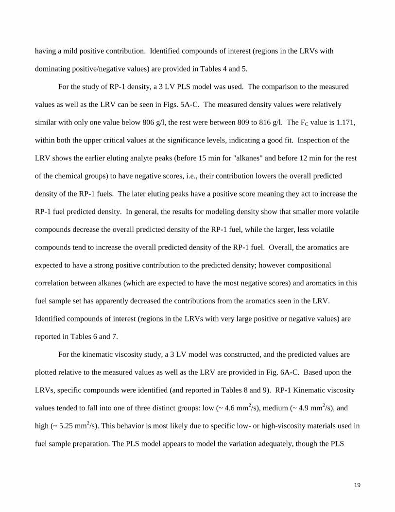
For iso-alkanes, the predicted mass% values using a 3 LV model are plotted relative to the

measured mass% values in Fig. 3B. While the iso-alkanes have very similar mass% values for 9 out of

11 samples, making it very challenging to model using PLS, there is good agreement between the

measured and predicted mass% values. The best fit line has a slope of 0.9679, the RMSEC is 0.233

mass%, and the RMSEP is 0.452 mass%, and the calculated SR is 0.257 mass%. The PLS model

overpredicted by only ~ 1.2% relative to the measured mass% values. The FC value is 1.221; here as

with the n-alkanes, this result indicates good agreement between the values predicted from the PLS

model and the measured values, in the context of the ideal 1:1 line.

For cycloalkanes, Fig. 3C provides the 3 LV model predicted mass% values plotted relative to

the measured mass% values. Note the measured mass% generally are very similar across samples, again

making for a very challenging PLS model, with the mass% values tending to be clustered more between

35.1% and 38.0%. Here too, the mass% values are spread across a little over one order of magnitude,

and yet the model matches the measured values extremely well. The line fit has a slope of 0.9847, the

RMSEC is 0.483 mass%, the RMSEP is 1.171 mass%, and the SR is 0.529 mass%. The FC value is

16

1.197, which is well below the upper critical values.

For di-cycloalkanes, the 3 LV model predicted mass% comparison to the measured mass% is

shown in Fig. 3D. The mass% values span between 13.6% and 18.7%, meaning the chemical variation

between any two samples is at most 5.1% with respect to the content of di-cycloalkanes. Even with this

challenging situation, the PLS model provides a best fit slope of 0.9705, which is still close to the ideal

slope of unity. The RMSEC is 0.251 mass%, the RMSEP is 0.355 mass%, and the calculated SR is

0.279 mass%. The FC value is 1.236, again well below the upper critical values.

For the tri-cycloalkanes in Fig. 3E a 3 LV PLS model was used, with the predicted mass% values

plotted relative to the measured mass% values. The predicted values appear to generally match well

with the measured values. This was an extremely challenging case because the variation was extremely

small between samples, only 1.2%, making a mass% deviation as little as 0.2% appear significant. The

slope of best fit line is 0.9426. The RMSEC is 0.102 mass%, the RMSEP is 0.184 mass%, and the SR is

0.109 mass%. The F-test value is 1.144, suggesting the predicted values are nearly equivalent to the

measured values.

Finally, for aromatics a 3 LV PLS model was used, and the comparison between the predicted

mass% and the measured mass% is shown in Fig. 3F. Even though the fuels analyzed exhibited a

bimodal distribution of aromatic content (most samples contained ~ 0.2%, with two samples containing

~ 3.6% and one sample containing 3.7%), the PLS model provides an excellent prediction of mass%

relative to the measured mass% values. The best fit line is 0.9955, and RMSEC, RMSEP and SR are

0.102 mass%, 0.237 mass%, and 0.113 mass%, respectively. The FC value is 1.217, indicating the

predicted values are essentially equivalent to the measured values.

The main point of section 3.2 on chemical composition studies is to demonstrate that the GC ×

GC – TOFMS data was readily correlated, via PLS modeling, to previously collected ASTM measured

17

quantitative hydrocarbon type data. This in turn provides us confidence that PLS modeling of the GC ×

GC – TOFMS data would be able to address more challenging and interesting studies, specifically,

correlations to physical properties with direct inference back to chemical compound identification

related to physical property relationships, as are explored in the next section.

3.3. Physical property studies using PLS

PLS modeling was performed on several measured chemical and physical properties (hydrogen

content, density, kinematic viscosity, net heat of combustion, sulfur content, sustained boiling

temperature, and vapor rise temperature) with results provided in Figs. 4-8. For reference, a figure key

and summary of the metrics for all the PLS models presented herein can be found in Table 3. The PLS

model prediction for the designated measured properties are provided in Figs. 4-8, and the LRVs of

selected properties are also provided (those include hydrogen content, density, kinematic viscosity, and

net heat of combustion; the LRVs of other modeled properties were omitted for brevity). Tables 4-11

contain lists of identified compounds based on respective LRVs. Referring to the PLS (3LV) model

plots of Figs. 4-8, as with the chemical compositional analysis in the previous section, the x-axis

displays the measured property values and the y-axis displays the PLS model predicted values. The

LRVs of PLS models offer complementary information to the values predicted by the PLS models

relative to the measured results. Each LRV was imported back into the base MATLAB workspace

(from PLS_Toolbox) where it was refolded to recover the dimensions of the 2D separation.

A review of PLS modeling is provided, so the reader can better understand how the modeling

relates to chemical compositional information. A linear combination of the LVs forms the LRV. By dot

product multiplication of a LRV (scores vector) with a given chromatogram for a sample (X-block

vector), a predicted property value (a scalar) is obtained. Thus, each intensity value for a given mass-to-

charge ratio (m/z) at a specific chromatographic time point in the LRV is a score which indicates the

18

contribution (sign and magnitude) of the compound(s) with respect to predicting a given property. To

view the LRVs more easily, the data is refolded into a 2D separation format, with the mass spectral

dimension summed, forming a LRV image similar to a 2D chromatogram. With the LRVs, we can now

explore the contribution of the chemical composition with respect to the physical properties in more

detail. Enclosed chemical groups (in Figs. 4B, 4C, 5B, 5C, 6B, 6C, 7B and 7C) are compared with

respect to specific chemical groups in various LRV plots.

The PLS (3 LV) model predicted values plotted relative to the measured values for hydrogen

content (weight%) are shown in Fig. 4A, and the LRV is shown in two parts for clarity. Fig. 4B shows

the positive contributions to the LRV, while Fig. 4C shows the negative contributions. The results in

Fig. 4A show the PLS model is a good fit, with a best fit line slope of 0.9401. The FC is 1.148 (well

below the upper critical values), indicating good agreement between the values predicted from the PLS

model and the measured values, in the context of the ideal 1:1 line, as defined in Eq. (4). In the LRV,

Figs. 4B and 4C, the aromatics (mono-, and di-) all have a negative score, meaning their contribution to

the PLS model decreases the predicted hydrogen content of RP-1 fuel, which is anticipated since

aromatics are not saturated in hydrogen (have a lower wt% contributed to hydrogen) relative to alkanes.

The alkane group has the earlier eluting compounds predominantly contributing to increasing the

hydrogen content, while most of the alkanes eluting from 15 to 25 min decrease the predicted hydrogen

content, as expected. Surprisingly, some of the later eluting compounds show a weak positive

contribution to the predicted value; this may be explained by the inadvertent correlation between

aromatics and alkanes eluting between those time intervals, which could occur if certain materials used

in the production of the fuel sample set were simultaneously abundant in particular hydrocarbon classes

(e.g., aromatics and alkanes). With respect to the cycloalkanes and di- and tri- cycloalkanes groups,

negative contributions for peaks are observed between 13 and 20 min with compounds outside this range

19

having a mild positive contribution. Identified compounds of interest (regions in the LRVs with

dominating positive/negative values) are provided in Tables 4 and 5.

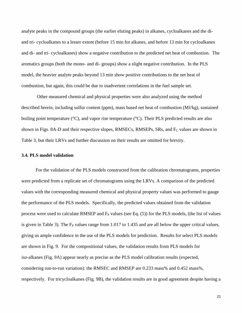
For the study of RP-1 density, a 3 LV PLS model was used. The comparison to the measured

values as well as the LRV can be seen in Figs. 5A-C. The measured density values were relatively

similar with only one value below 806 g/l, the rest were between 809 to 816 g/l. The FC value is 1.171,

within both the upper critical values at the significance levels, indicating a good fit. Inspection of the

LRV shows the earlier eluting analyte peaks (before 15 min for "alkanes" and before 12 min for the rest

of the chemical groups) to have negative scores, i.e., their contribution lowers the overall predicted

density of the RP-1 fuels. The later eluting peaks have a positive score meaning they act to increase the

RP-1 fuel predicted density. In general, the results for modeling density show that smaller more volatile

compounds decrease the overall predicted density of the RP-1 fuel, while the larger, less volatile

compounds tend to increase the overall predicted density of the RP-1 fuel. Overall, the aromatics are

expected to have a strong positive contribution to the predicted density; however compositional

correlation between alkanes (which are expected to have the most negative scores) and aromatics in this

fuel sample set has apparently decreased the contributions from the aromatics seen in the LRV.

Identified compounds of interest (regions in the LRVs with very large positive or negative values) are

reported in Tables 6 and 7.

For the kinematic viscosity study, a 3 LV model was constructed, and the predicted values are

plotted relative to the measured values as well as the LRV are provided in Fig. 6A-C. Based upon the

LRVs, specific compounds were identified (and reported in Tables 8 and 9). RP-1 Kinematic viscosity

values tended to fall into one of three distinct groups: low (~ 4.6 mm2/s), medium (~ 4.9 mm

2/s), and

high (~ 5.25 mm2/s). This behavior is most likely due to specific low- or high-viscosity materials used in

fuel sample preparation. The PLS model appears to model the variation adequately, though the PLS

20

model seems to over predict and under predict some values more than the other models. As with the

other physical property models, statistical results are provided in Table 3. Ironically, the FC is 1.096, the

lowest FC value recorded, indicating this is a very accurate model overall. The LRV for kinematic

viscosity draws great similarity to the LRV for the measured density (split into positive and negative

portions in Figs. 6B and 6C, though with some noticeable differences. In the positive values (LRV),

there are literally no major contributions from the cyclic groups between 10 and 15 min, whereas the

majority of peaks appear between 15 and 25 min. Meanwhile in the negative portion of the regression

vector, there are more contributions from the alkane group, as well as significantly more peaks from the

cycloalkane, and di- and –tri cycloalkane groups. As expected, smaller, more volatile compounds (in

this case, eluting at around 5 to 15 min on the first column) have negative scores, therefore (according to

the PLS model) contribute to lowering the RP-1 fuel kinematic viscosity, while heavier compounds

eluting after 17 min have positive scores and tend to raise the RP-1 fuel overall predicted kinematic

viscosity. Interestingly, the aromatic groups show little contribution. Identified compounds of interest

(regions in the LRVs with dominating positive/negative values) are identified in Tables 8 and 9.

The results for the PLS model (3 LV) constructed for volume-based net heat of combustion

(MJ/l) are provided in Table 3, and the predicted values are plotted relative to the measured values as

well as the LRV are provided in Fig. 7A-C. Identified compounds of interest are found in Tables 10 and

11. Though the PLS model predicted net heat of combustion values Fig. 7A show a strong agreement

with the measured ASTM values, with a slope of 0.9691. Once again it is important to note the scale:

the data ranges from 34.47 to 34.89 MJ/l (less than 0.5 MJ/l). With net heat of combustion (MJ/l), as

with many other properties studied herein, both the composition of the RP samples and the measured

ASTM values are very similar, making it more challenging to model with PLS. The corresponding LRV,

shown in Figures 7B and 7C, bares similarity to the LRV for the density model: In general, more volatile

21

analyte peaks in the compound groups (the earlier eluting peaks) in alkanes, cycloalkanes and the di-

and tri- cycloalkanes to a lesser extent (before 15 min for alkanes, and before 13 min for cycloalkanes

and di- and tri- cycloalkanes) show a negative contribution to the predicted net heat of combustion. The

aromatics groups (both the mono- and di- groups) show a slight negative contribution. In the PLS

model, the heavier analyte peaks beyond 13 min show positive contributions to the net heat of

combustion, but again, this could be due to inadvertent correlations in the fuel sample set.

Other measured chemical and physical properties were also analyzed using the method

described herein, including sulfur content (ppm), mass based net heat of combustion (MJ/kg), sustained

boiling point temperature (°C), and vapor rise temperature (°C). Their PLS predicted results are also

shown in Figs. 8A-D and their respective slopes, RMSECs, RMSEPs, SRs, and FC values are shown in

Table 3, but their LRVs and further discussion on their results are omitted for brevity.

3.4. PLS model validation

For the validation of the PLS models constructed from the calibration chromatograms, properties

were predicted from a replicate set of chromatograms using the LRVs. A comparison of the predicted

values with the corresponding measured chemical and physical property values was performed to gauge

the performance of the PLS models. Specifically, the predicted values obtained from the validation

process were used to calculate RMSEP and FP values (see Eq. (5)) for the PLS models, (the list of values

is given in Table 3). The FP values range from 1.017 to 1.435 and are all below the upper critical values,

giving us ample confidence in the use of the PLS models for prediction. Results for select PLS models

are shown in Fig. 9. For the compositional values, the validation results from PLS models for

iso-alkanes (Fig. 9A) appear nearly as precise as the PLS model calibration results (expected,

considering run-to-run variation): the RMSEC and RMSEP are 0.233 mass% and 0.452 mass%,

respectively. For tricycloalkanes (Fig. 9B), the validation results are in good agreement despite having a

22

noticeably greater spread of predicted values: the RMSEC and RMSEP are 0.102 mass% and 0.184

mass%, respectively. Also shown are the validation results for hydrogen content (Fig. 9C) and density

(Fig. 9D), both showing very similar values with respect to the calibration results, their respective

RMSEP are 0.024 wt% and 0.862 (g/l).

4. Conclusions

The rocket kerosene study presented herein has demonstrated separation of the compounds in

RP-1 fuel using GC × GC – TOFMS with a reversed column configuration (RTX-wax primary column

coupled to a RTX-1 secondary column), followed by chemometric analysis using PLS and the

identification of analyte peaks using ChromaTOF, nontarget PARAFAC, and then the NIST-MS library.

The GC × GC column configuration implemented has demonstrated the ability to resolve many analyte

peaks. Moreover, the separation distinguishes not only between groups of hydrocarbon compound

classes, but also between many distinct analyte compounds. PLS modeling was performed on the GC ×

GC – TOFMS data to analyze chemical composition with a targeted focus of drawing connections

between the compounds separated in the 2D chromatograms and measured chemical and physical

properties of the fuel. In spite of the fact that some chemical groups exhibited compositional correlation

(likely an artifact of fuel preparation involving blending of available feed stocks) with other chemical

groups for certain measured values in the PLS models, the models show excellent prediction ability for

mass% composition values of hydrocarbon groups based on their GC × GC – TOFMS chromatograms.

The root mean square error values found in Table 3 (as measures of precision) can be compared

to the reported uncertainty values accompanying the respective ASTM measurement methods. For

example, ASTM D4052, the standard test method for density, reports precision of 0.52 g/l

(reproducibility) and bias of 0.6 g/l [36]. The RMSEC of the PLS model for density was determined in

our study to be 0.55 g/l, which is similar to the uncertainty in the reference method. Likewise, kinematic

23

viscosity as measured with ASTM D455 has a reported reproducibility of 0.092 mm2/s (a value for bias

was not given) [37]. In comparison, the RMSEC in the PLS model for kinematic viscosity was

determined to be 0.072 mm2/s. Finally, the method for net heat of combustion (ASTM D4809) reports a

reproducibility of 0.324 MJ/kg and a bias of 0.089 MJ/kg [38]. The RMSEC of the PLS model for net

heat of combustion was determined to be only 0.009 MJ/kg in our study. Note that PLS assumes no error

in the measurements given in the Y-block and that any error in those measurements would necessarily

affect the error in the model.

Ideally, for chemical composition, each chemical group measurement would correspond to an

exclusive chemical group showing positive scores. However, achieving such a result would require a

greater collection of different fuel samples with diversity in chemical composition in order to minimize

any observable correlation between chemical groups. Any observed correlation may suggest that the

LRVs need to be inspected more carefully and that caution should be exercised when drawing

connections between measured values and chromatographic/chemical information. Identifying

compounds that contribute positively and negatively to the property in question can aid in the

interpretation of LRVs by substantiating the identification of influencing hydrocarbon groups and

confirming the compositional correlation between modeled fuel samples.

The F-test values overall (FC and FP) are all slightly above 1, indicating good overall agreement

between the measured, modeled and predicted values. Though the full analysis of the error of the PLS

models is beyond the scope of this study, the use of replicate chromatograms produced similar predicted

values. A more expanded investigation using temperature-dependent physical properties [39], and use

of PLS to predict those values will be the subject of an upcoming future papers.

24

Acknowledgement

The work at the University of Washington (UW) was performed under subcontract to ERC,

Incorporated, Air Force Research Laboratory, Edwards AFB, CA. The fuels were provided by the Air

Force Research Laboratory/RQRC, Edwards AFB, CA. Hydrocarbon type analysis was performed by

Dr. Linda Shafer of the University of Dayton Research Institute (UDRI), Wright-Patterson AFB, OH.

Certain commercial equipment, instruments or materials are identified in this paper in order to

adequately specify the experimental procedure. Such identification does not imply recommendation or

endorsement by the University of Washington, the United States Air Force, or the National Institute of

Standards and Technology, nor does it imply that the materials or equipment identified are necessarily

the best available for that purpose.

REFERENCES

[1] D. Cookson, B. Smith, Energy Fuels 24 (1990) 152.

[2] G. Liu, L. Wang, H. Qu, H. Shen, X. Zhang, S. Zhang, Z. Mi, Fuel 86 (2007) 2551.

[3] M. L. Huber, E. W. Lemmon, T. J. Bruno, Energy Fuels 23 (2009) 5550.

[4] M. J. DeWitt, T. Edwards, L. Shafer, D. Brooks, R. Striebich, S. P. Bagley, M. J. Wornant, Ind. Eng.

Chem. Res. 50 (2011) 10434.

[5] M. C. Billingsley, J. T. Edwards, L. M. Shafer, T. J. Bruno, AIAA 2010-6824, 46th American

Institute of Aeronautics and Astronautics (AIAA) Joint Propulsion Conference and Exhibit, Nashville,

TN (July 2010).

[6] T. M. Lovestead, B. C. Windom, J. R. Riggs, C. Nickell, T. J. Bruno, Energy Fuels 24 (2010) 5611.

[7] R. V. Gough, T. J. Bruno, Energy Fuels 27 (2013) 294.

[8] P. Y. Hsieh, K. R. Abel, T. J. Bruno, Energy Fuels 27 (2013) 804.

[9] J. L. Burger, T. J. Bruno, Energy Fuels 26 (2012) 3661.

25

[10] N. J. Begue, J. A. Cramer, C. Von Bargen, K. M. Myers, K. J. Johnson, R. E. Morris, Energy Fuels

25 (2011) 1917.

[11] T. J. Bruno, L. S. Ott, T. M. Lovestead, M. L. Huber, J. Chromatogr. A (Extraction 2009 Special

Issue), Invited Review, 1217 (2010) 2703.

[12] J. S. Nadeau, B. W. Wright, R. E. Synovec, Talanta 81 (2010) 120.

[13] R. B. Wilson, W. C. Siegler, J. C. Hoggard, B. D. Fitz, J. S. Nadeau, R. E. Synovec, J. Chromatogr.

A 1218 (2011) 3130.

[14] J. H. Christensen, G. Tomasi, A. B. Hansen, Environ. Sci. Technol. 39 (2005) 255.

[15] J. L. Hope, A. E. Sinha, B. J. Prazen, R. E. Synovec, J. Chromatogr. A, 1086 (2005) 185.

[16] R. E. Mohler, K. M. Dombek, J. C. Hoggard, E. T. Young, R. E. Synovec, Anal. Chem. 78 (2006)

2700.

[17] K. M. Pierce, J. C. Hoggard, R. E. Mohler, and R. E. Synovec, J. Chromatogr. A 1184 (2008) 341.

[18] J. C. Hoggard, R. E. Synovec, Anal. Chem. 80 (2008) 6677.

[19] C. G. Fraga, B. J. Prazen, R. E. Synovec, Anal. Chem. 72 (2000) 4154.

[20] B. J. Prazen, K. J. Johnson, A. Weber, R. E. Synovec, Anal. Chem. 73 (2001) 5677.

[21] K. J. Johnson, R. E. Synovec, J. Chemom. Intell. Lab. Syst. 60 (2002) 225.

[22] K. J. Johnson, B. J. Prazen, D. C. Young, Synovec R. E., J. Sep. Sci. 27 (2004) 410.

[23] K. M. Pierce, B. Kehimkar, L. C. Marney, J.C. Hoggard, R. E. Synovec, J. Chromatogr. A 1255

(2012) 3.

[24] B. Omais, M. Courtiade, N. Charon, D. Thiébaut, A. Quignard, M. C. Hennion, J. Chromatogr.

A 1218 (2011) 3233.

[25] B. Omais, M. Courtiade, N. Charon, D. Thiébaut, A. Quignard, M. C. Hennion, J. Chromatogr. A

1218 (2011) 3233.

[26] R. E. Mohler, K. M. Dombek, J. C. Hoggard, K. M. Pierce, E. T. Young, R. E. Synovec, Analyst

132 (2007) 756.

[27] K. M. Pierce, J. C. Hoggard, J. L. Hope, P. M. Rainey, A. N. Hoofnagle, R. M. Jack, B. W. Wright,

R. E. Synovec, Anal. Chem. 78 (2006) 5068.

[28] J. C. Hoggard, W. C. Siegler, R. E. Synovec, J.chemom. 23 (2009) 421.

26

[29] F. Westad, N. K. Afseth, R. Bro, Anal. Chim. Acta. 595 (2007) 323.

[30] T. Rajalahti, O. M. Kvalheim, Int. J. Pharm. 417 (2011) 280.

[31] A. A. Gowen, G. Downey, C. Esquerre, C. P. O'Donnell, J. Chemom. 25 (2011) 375.

[32] J. C. Hoggard, http://synoveclab.chem.washington.edu/Jamin.htm.

[33] G. D. Christian, Analytical Chemistry, John Wiley & sons, Hoboken NJ, 6th ed., 2004.

[34] R. E. Synovec, Anal. Chem. 59 (1987) 2877.

[35] P. R. Bevington, Data Reduction and Error Analysis for the Physical Sciences, McGraw-Hill, New

York, 1969.

[36] ASTM Standard D4052, 1981 (2011), “Standard Test Method for Density, Relative Density, and

API Gravity of Liquids by Digital Density Meter,” ASTM International, West Conshohocken, PA 2011,

DOI: 10.1520/D4052-11, www.astm.org.

[37] ASTM Standard D455, 1937 (2012), “Standard Test Method for Kinematic Viscosity of

Transparent and Opaque Liquids(and Calculation of Dynamic Viscosity),” ASTM International, West

Conshohocken, PA 2012, DOI: 10.1520/D455-12, www.astm.org.

[38] ASTM Standard D4809, 1988 (2013), “Standard Test Method for

Heat of Combustion of Liquid Hydrocarbon Fuels by Bomb

Calorimeter (Precision Method),” ASTM International, West Conshohocken, PA 2012, DOI:

10.1520/D4809-13, www.astm.org.

[39] T. J. Fortin, Energy Fuels 26 (2012) 4383.

27

Figure Captions

Fig. 1. RP-1 GC × GC – TOFMS total ion current (TIC) chromatograms, collected using a 30 m Rtx-

wax column for the first separation dimension followed by a 1.2 m Rtx-1 column for the second

separation dimension at a constant inlet pressure of 35 psig (241 kPa). Chemical groups are indicated

and annotated. (A) RP-1 LB073009-05. (B) RP-1 LB073009-09. (C) RP-1 XC2521HW10. (D)

Template used for aforementioned group boundaries for chemical groups. Dots signify locations of

identified compound peaks used in defining the group boundaries. For visualization purposes, the

numbers correspond to selected analyte peaks, found in Table 2. The other dots also correspond to

compounds in Table 2 but are not numbered for clarity. (E) TIC chromatogram of LB073009-05

summed on the second column dimension, simulating a 1D-GC-MS separation.

Fig. 2. (A) GC × GC – TOFMS chromatogram for selective ion m/z 105 of RP-1 LB073009-05. (B)

Magnification of selected region of (A). (C) GC × GC – TOFMS m/z 136 chromatogram of RP-1

LB073009-05, where the adamantane peak is identified.

Fig. 3. Comparison between the predicted hydrocarbon class values (mass%) derived from the GC ×

GC-TOFMS with PLS models and the measured values obtained using their respective measured values,

with the dashed line representing an ideal agreement between the predicted and measured values and the

solid line representing the linear regression best fit line. (A) n-alkanes (ASTM D2425 with ‘n-alkane

analysis’) using a 3 LV PLS model. (B) iso-alkanes (ASTM D2425) using a 3 LV PLS model. (C)

cycloalkanes (ASTM D2425) using a 3 LV PLS model. (D) di-cycloalkanes (ASTM D2425) using a 3

LV PLS model. (E) tri-cycloalkanes (ASTM D2425) using a 3 LV PLS model. (F) aromatics (ASTM

D6379) using a 3 LV PLS model.

28

Fig. 4. Results of the 3 LV PLS model for hydrogen content. (A) Hydrogen content (wt%) predicted

values plotted relative to the measured values (Perkin Elmer Elemental Analyzer, Model EA2400). The

dashed line represents an ideal agreement between the predicted and measured values and the solid line

represents the linear regression best fit line. (B) Hydrogen content LRV 2D plot, positive values only.

(C) Hydrogen content LRV 2D plot, negative values only.

Fig. 5. Results of the 3 LV PLS model for density. (A) Density (g/l) predicted values plotted relative to

the measured values (ASTM D4052). The dashed line represents an ideal agreement between the

predicted and measured values and the solid line represents the linear regression best fit line. (B)

Density LRV, positive values only. (C) Density LRV, negative values only.

Fig. 6. Results of the 3 LV PLS model for kinematic viscosity. (A) Kinematic viscosity (mm2/s)

predicted values plotted relative to the measured values (ASTM D445). The dashed line represents an

ideal agreement between the predicted and measured values and the solid line represents the linear

regression best fit line. (B) Kinematic viscosity LRV, positive values only. (C) Kinematic viscosity

LRV, negative values only.

Fig. 7. Results of the 3 LV PLS model for net heat of combustion (MJ/l). (A) Net heat of combustion

(MJ/l) predicted values plotted relative the measured values (ASTM D4809). The dashed line represents

an ideal agreement between the predicted and measured values and the solid line represents the linear

regression best fit line. (B) Kinematic viscosity LRV, positive values only. (C) Kinematic viscosity

LRV, negative values only.

29

Fig. 8. Results of other 3 LV PLS models for various measured properties. The dashed line represents

an ideal agreement between the predicted and measured values and the solid line represents the linear

regression best fit line. (A) Net heat of combustion (MJ/kg) predicted plotted relative to the measured

values (ASTM D4809). (B) Sulfur content (ppm) predicted values plotted relative to the measured

values (using SCD). (C) Sustained boiling temperature (°C ) predicted values plotted relative to the

measured values. (D) Vapor rise temperature (°C ) predicted values plotted relative to the measured

values.

Fig 9. Validation results for selected aforementioned PLS models. (A) Validation results for the iso-

alkanes PLS model. (B) Validation results for the tricycloalkanes PLS model. (C) Validation results for

the hydrogen content PLS model. (D) Validation results for the density PLS model.

30

Tables

Table 1. RP-1 Fuel Set, where the RP-1 Sample number is used herein, while the NIST and AFRL

numbers are provided for reference to previous studies of interest.

RP-1 Sample

NIST Number

[6]

AFRL Designation

[5]

1 11 LB080409-01

2 10 LB073009-06

3 9 LB073009-08

4 8 LB080409-05

5 7 LB073009-05

6 6 LB073009-10

7 5 LB073009-01

8 4 LB073009-09

9 1 LB073009-02

10 2 LB073009-03

11 3 XC2521HW10

31

Table 2. Template data with the assigned number (#) used in Fig. 1D, of each representative identified

compound with their retention times on column one (1tR) and two (

2tR) in s, and mass spectral match

value (MV). This information was used to define the encircled various chemical groups.

# Compound Identification 1tR (min)

(s)(s(sec)

2tR(s)

(s)(sec)

MV Chemical groups

1 Nonane 5.96 1.65 911 alkanes

2 Methylnonane 7.42 1.92 925 alkanes

3 Decane 8.25 1.93 950 alkanes

4 Undecane 10.83 2.03 946 alkanes

5 Dimethyldecane (or dodecane) 10.83 2.23 902 alkanes

6 Dodecane 13.5 2.06 941 alkanes

7 Tetradecane 18.63 2.04 959 alkanes

8 Pentadecane 20.92 1.95 938 alkanes

9 Hexadecane 23.167 1.91 920 alkanes

10 Pristane 24.42 2.11 921 alkanes

11 Trimethylcyclohexane 5.29 1.33 911 cycloalkanes

12 Cyclohexane, 1,1,2,3-tetramethyl-

(isomer)

8.58 1.53 881 cycloalkanes

13 Cyclohexane, 1,1,2,3-tetramethyl- 9.21 1.52 840 cycloalkanes

14 Cyclohexane, pentyl- 13.33 1.67 843 cycloalkanes

15 Cyclohexane, 1-methyl-4-(1-

methylbutyl)-

14.38 1.70 881 cycloalkanes

16 Cyclohexane, hexyl- 16.13 1.64 901 cycloalkanes

17 Heptylcyclohexane 18.79 1.59 869 cycloalkanes

18 Cyclotetradecane 21.13 1.62 858 cycloalkanes

19 Cyclohexane, octyl- 21.29 1.60 882 cycloalkanes

20 n-Nonylcyclohexane 23.63 1.60 929 cycloalkanes

21 2-Methyloctahydropentalene 8.58 1.30 914 di- & tri-cycloalkanes

22 Bicyclo[2.2.1]heptane, trimethyl-

(C10H18) 8.83 1.41 806 di- & tri-cycloalkanes

23 1H-Indene, octahydro-, cis- 11.17 1.24 930 di- & tri-cycloalkanes

24 Naphthalene, decahydro-, trans- 12.83 1.31 944 di- & tri-cycloalkanes

25 Adamantane 15 1.17 962 di- & tri-cycloalkanes

26 Naphthalene, decahydro-2,6-dimethyl- 15.04 1.47 880 di- & tri-cycloalkanes

27 2-Methyladamantane 17.25 1.19 871 di- & tri-cycloalkanes

28 Bicyclohexyl 20 1.30 890 di- & tri-cycloalkanes

29 Trans-hexamethyl-octahydro-1H-Indene

(C15H28) 22.25 1.40 820 di- & tri-cycloalkanes

30 Tricyclo[4.2.2.0(2,5)]dec-7-ene, 7-butyl- 27.03 1.12 820 di- & tri-cycloalkanes

31 Toluene 9.5 0.75 952 mono-aromatics

32 Ethylbenzene 11.88 0.82 953 mono-aromatics

33 Xylene 12.08 0.82 960 mono-aromatics



36 Ethyl trimethyl benzene 17.21 0.91 902 mono-aromatics

37 Isobutyltoluene 17.21 0.98 914 mono-aromatics

38 Trimethylbenzene 17.5 0.84 950 mono-aromatics

39 Methyltetralin 25.83 0.87 928 mono-aromatics

40 Dimethyltetralin 27.96 0.89 915 mono-aromatics

32

41 Naphthalene 26.83 0.76 905 di-aromatics

42 Methyl naphthalene 29 0.78 900 di-aromatics

43 Methyl naphthalene (isomer) 29.75 0.80 902 di-aromatics

44 Dimethyl naphthalene 31.08 0.83 931 di-aromatics

45 Dimethyl naphtalene (isomer) 31.83 0.83 921 di-aromatics

46 Methyldiphenyl (methyl phenyl benzene) 33.33 0.83 909 di-aromatics

47 Trimethyl naphthalene 34.42 0.89 939 di-aromatics

33

Table 3. Summary of PLS model metrics for measured properties analyzed. Metrics (slope, RMSEC,

RMSEP, SR, FC and FP values) are provided in the context of the relevant figures.

Measured Property Figures slope RMSEC RMSEP SR FC FP

n-alkanes (mass%) 3A 0.9879 0.457 0.648 0.497 1.180 1.091

iso-alkanes (mass%) 3B 0.9679 0.233 0.452 0.257 1.221 1.102

Cycloalkanes (mass%) 3C 0.9847 0.483 1.171 0.529 1.197 1.087

Dicycloalkanes (mass%) 3D 0.9705 0.251 0.355 0.279 1.236 1.063

Tricycloalkanes (mass%) 3E 0.9426 0.102 0.184 0.109 1.144 1.327

Aromatics (mass%) 3F 0.9955 0.102 0.237 0.113 1.217 1.017

Hydrogen Content (wt%) 4A-C 0.9401 0.019 0.024 0.020 1.148 1.145

Density (g/l) 5A-C 0.9590 0.550 0.862 0.596 1.171 1.072

Kinematic Viscosity (mm2/s) 6A-C 0.9255 0.072 0.111 0.075 1.096 1.162

Net Heat of Combustion

(MJ/l) 7A-C 0.9691 0.021 0.032 0.023 1.161 1.037

Net Heat of Combustion

(MJ/kg) 8A 0.9542 0.009 0.013 0.010 1.178 1.435

Sulfur (ppm) by SCD 8B 0.9426 1.734 2.756 1.861 1.151 1.119

Sustained boiling temp. (°C) 8C 0.9851 0.286 0.536 0.314 1.205 1.126

Vapor rise temp. (°C) 8D 0.9661 0.410 0.650 0.525 1.640 1.149

34

Table 4. Major contributing compounds identified in LRVs for hydrogen content (positive) per Fig. 4B.

# Compound Identification 1tr(min) 2

tr(s) MV Chemical group

1 Decane (C10H22) 8.25 1.98 875 alkanes

2 Undecane (C11H24) 10.92 2.1 954 alkanes

3 2,6-Dimethyldecane (C12H26) 10.92 2.32 910 alkanes

4 Cyclohexane, 1,2-diethyl-, cis- (C10H20) 8.33 1.64 864 cycloalkanes

5 Cyclohexane, (2-methyl-1-propenyl)- (C10H18) 11.17 1.4 875 cycloalkanes

6 Cyclic (formula unkown) 20 1.68 750+ cycloalkanes

7 Bicyclohexyl (C12H22) 20 1.34 886 di-& tri-

cycloalkanes 8 Decahydro-pentamethylnaphthalene (C15H28) 23.5 1.4 807 di-& tri-

cycloalkanes 9 no significant peak found

* mono-aromatics

10 no significant peak found di-aromatics

* “No significant peak found” indicates no analytes contribute significantly from that chemical group.

Table 5. Major contributing compounds identified in LRVs for hydrogen content (negative) per Fig. 4C.



1 Tridecane, 7-methyl- (C14H30) 14.75 2.38 805 alkanes

2 Tridecane (C13H28) 16.17 2.08 946 alkanes

3 Tetradecane (C14H30) 16.17 2.2 910 alkanes

4 Isobutyl-Dimethylcyclohexane (C12H24) 13.58 1.74 818 cycloalkanes

5 C12H24 alkylated cycloalkane 14.67 1.72 750+ cycloalkanes

6 Cyclohexane, (3-methylpentyl)- (C12H24) 15.17 1.68 888 cycloalkanes

7 Naphthalene, decahydro-2-methyl- (C11H20) 14.75 1.42 923 di-&tri-

cycloalkanes 8 Decalin, syn-1-methyl-, cis- (C11H20) 16.67 1.32 924 di-&tri-

cycloalkanes 9 Naphthalene, 1,2,3,4-tetrahydro- (C10H12) 22.25 0.86 957 mono-aromatics

10 Naphthalene, 1,2,3,4-tetrahydro-6-methyl- (C11H14) 24.58 0.9 928 mono-aromatics

11 Benzene, cyclohexyl- (C12H16) 25.33 0.94 928 mono-aromatics

12 Naphthalene (C10H8) 36.83 0.78 902 di-aromatics

13 Dimethylnaphthalene (C12H12) (isomer) 31.67 0.84 934 di-aromatics

14 Dimethylnaphthalene (C12H12) 31.83 0.84 920 di-aromatics

Table 6. Major contributing compounds identified in LRVs for density (positive) per Fig. 5B.



1 Undecane, 2,6-dimethyl- (C13H28) 13.42 2.32 880 alkanes

2 Tridecane, 7-methyl- (C14H30) 14.75 2.38 818 alkanes

3 Dodecane, 2,6,10-trimethyl- (C15H32) 17.5 2.24 882 alkanes

4 Cyclohexane, 1-ethyl-2-propyl- (C11H22) 11.92 1.72 835 cycloalkanes

5 Cyclohexane, 1-methyl-4-(1-methylethyl)-, cis- (C10H20) 17.08 1.72 831 cycloalkanes

6 Heptylcyclohexane (C13H26) 18.83 1.66 872 cycloalkanes


cycloalkanes 8 Adamantane, dimethyl- (C12H20) 14.75 1.42 888 di-&tri-

cycloalkanes

35

9 Decalin, syn-1-methyl-, cis- (C11H20) 16.67 1.32 819 di-&tri-

cycloalkanes 10 no significant peak found mono-aromatics


Table 7. Major contributing compounds identified in LRVs for density (negative) per Fig. 5C.



1 Decane (C10H22) 8.25 1.98 953 alkanes


3 Dodecane (C12H26) 10.92 2.32 864 alkanes

4 Cyclohexane, diethyl- (isomer)(C10H20) 7.67 1.62 873 cycloalkanes


6 C10H18 11.17 1.4 800+ di-&tri-

cycloalkanes 7 Xylene (C8H10) 12.25 0.82 913 mono-aromatics




Table 8. Major contributing compounds identified in LRVs for kinematic viscosity (positive) per Fig.

6B.

# Compound Identification 1tr (min)

2tr (s) MV Chemical group

1 Tetradecane 19.5 2.01 881 alkanes

2 Tetradecane, 2-methyl- 19.88 2.01 919 alkanes

3 4-Methyltridecane 17.42 2.05 910 alkanes

4 1-Cyclohexylheptane 18.79 1.62 863 cycloalkanes

5 1-Methyl-4-(1-methylbutyl)cyclohexane (C12H24) 19.63 1.68 812 cycloalkanes

6 Octylcyclohexane 21.29 1.6 880 cycloalkanes

7 alkane branched dicycloalkane (C15H28) 22.21 1.44 825 di- & tri- cycloalkanes

8 1,1'-Bicyclohexyl, 2-methyl-, cis- (C13H24) 20.83 1.36 818 di- & tri- cycloalkanes

9 Bicyclohexane 20 1.31 895 di- & tri- cycloalkanes

10 no significant peak found mono-aromatics


36

Table 9. Major contributing compounds identified in LRVs for kinematic viscosity (negative) per Fig.

6C.

# Compound Identification 1tr (min)

2tr (s) MV Chemical group

1 Undecane 10.88 2.06 953 alkanes

2 2,6-Dimethyldecane 10.88 2.268 914 alkanes

3 Decane 8.25 1.942 955 alkanes

4 1-Methyl-2-propylcyclohexane (C10H20) 8.92 1.65 866 cycloalkanes

5 Cyclohexane, 1-ethyl-1,3-dimethyl-, trans- (C10H20) 7.67 1.607 844 cycloalkanes

6 cis,trans-1,2,3-Trimethylcyclohexane 7.46 1.39 941 cycloalkanes

7 trans-Decahydronaphthalene (C10H18) 12.83 1.34 924 di- & tri- cycloalkanes

8 cis-octahydro-Indene (C9H16) 11.17 1.24 928 di- & tri- cycloalkanes

9 trans-octahydro-Indene (C9H16) 9.75 1.28 912 di- & tri- cycloalkanes

10 no significant peak found mono-aromatics


Table 10. Major contributing compounds identified in LRVs for volume based net heat of combustion

(MJ/l) (positive) per Fig. 7B.



1 Tridecane, methyl- (C14H30) 14.75 2.38 807 alkanes

2 2-Methyltridecane (C14H30) 17.5 2.26 925 alkanes

3 Dodecane, trimethyl- (C15H32) 19.42 2.24 856 alkanes

4 Cyclohexane, 1-methyl-4-(1-methylethyl)-, cis- (C10H20) 17.08 1.72 838 cycloalkanes

5 Cyclohexane, 1-ethyl-2-methyl-, cis- (C9H18) 17.58 1.7 817 cycloalkanes

6 Heptylcyclohexane (C13H26) 18.83 1.66 851 cycloalkanes

7 Methyldecahydronaphthalene (C11H20) 16.67 1.32 931 di-&tri-

cycloalkanes 8 2-Methyladamantane (C11H18) 17.33 1.22 870 di-&tri-

cycloalkanes 9 no significant peak found mono-aromatics


Table 11. Major contributing compounds identified in LRVs for net heat of combustion (MJ/l)

(negative) per Fig. 7C.



1 Decane isomer (C10H22) 8.25 1.98 944 alkanes


37

3 2,6-Dimethyldecane (C12H26) 10.92 2.32 910 alkanes

4 Cyclohexane, 1-ethyl-1,3-dimethyl-, trans- (C10H20) 7.67 1.62 845 cycloalkanes


6 1-Methyl-4-(1-methylethyl)-cyclohexane (C10H20) 8.92 1.7 882 cycloalkanes

7 Cyclohexane, (2-methyl-1-propenyl)- (C10H18) 11.17 1.4 863 cycloalkanes

8 Naphthalene, decahydro-2-methyl- (C11H20) 14.08 1.42 929 di- & tri-


10 Naphthalene, 1,2,3,4-tetrahydro- (C10H12) 22.25 0.86 960 mono-aromatics

11 Naphthalene, 2-methyl- (C11H10) 29.08 0.82 903 di-aromatics

12 2,6-Dimethylnaphthalene (C12H12) 31.83 0.84 920 di-aromatics

TIC: LB073009-05

5 10 15 20 25 30 35

0.5

1

1.5

2

2.5

Time, Column 1 (minutes)

alkanes

cycloalkanes

di- and tri- cylcoalkanes

mono-aromatics di-aromatics

Tim

e,

Colu

mn 2

(se

co

nd

s)

Figure 1A

Figure 1B

TIC: LB073009-09

alkanes


5 10 15 20 25 30 35

0.5

1

1.5

2

2.5


cycloalkanes


Tim

e,

Colu

mn 2

(se

co

nd

s)

Figure 1C

TIC: XC2521HW10

alkanes


5 10 15 20 25 30 35

0.5

1

1.5

2

2.5


cycloalkanes


Tim

e,

Colu

mn 2

(se

co

nd

s)

Figure 1D

TEMPLATE

alkanes

cycloalkanes


mono-aromatics

di-aromatics

1

2 3

11

12 13 22

21 23

32-35 31

5 10 15 20 25 30 35

0.5

1

1.5

2

2.5


Tim

e,

Colu

mn 2

(se

co

nd

s)

4

5

6 7 8 9

10

14 15 16 17 18 19 20

24 25 26

27 28 29

30

40 39

41-47

36-38

Figure 1E

0

4

8

12

16

20 x 106

Time (minutes)

Sig

nal in

ten

sity

TIC: LB073009-05 summed 2nd column dimension

5 10 15 20 25 30 35

Figure 2A

m/z 105: LB073009-05

alkanes


5 10 15 20 25 30 35

0.5

1

1.5

2

2.5


cycloalkanes


Tim

e,

Colu

mn 2

(se

co

nd

s)

Figure 2B

m/z 105 LB073009-05

18 19 20 21 22 0.8

0.9

1

1.1

1.2


Tim

e,

Colu

mn 2

(se

co

nd

s)

Figure 2C

m/z 136 LB073009-05

12 13 14 15 16 17 18 19 1

1.2

1.4

1.6

1.8

Adamantane


Tim

e,

Colu

mn 2

(se

co

nd

s)

Figure 3A

0 2 4 6 8 10 12 14 0

2

4

6

8

10

12

14

Mass% Measured

Ma

ss%

Pre

dic

ted

PLS model 1:1 Fit

n-alkanes,

PLS model 3LV

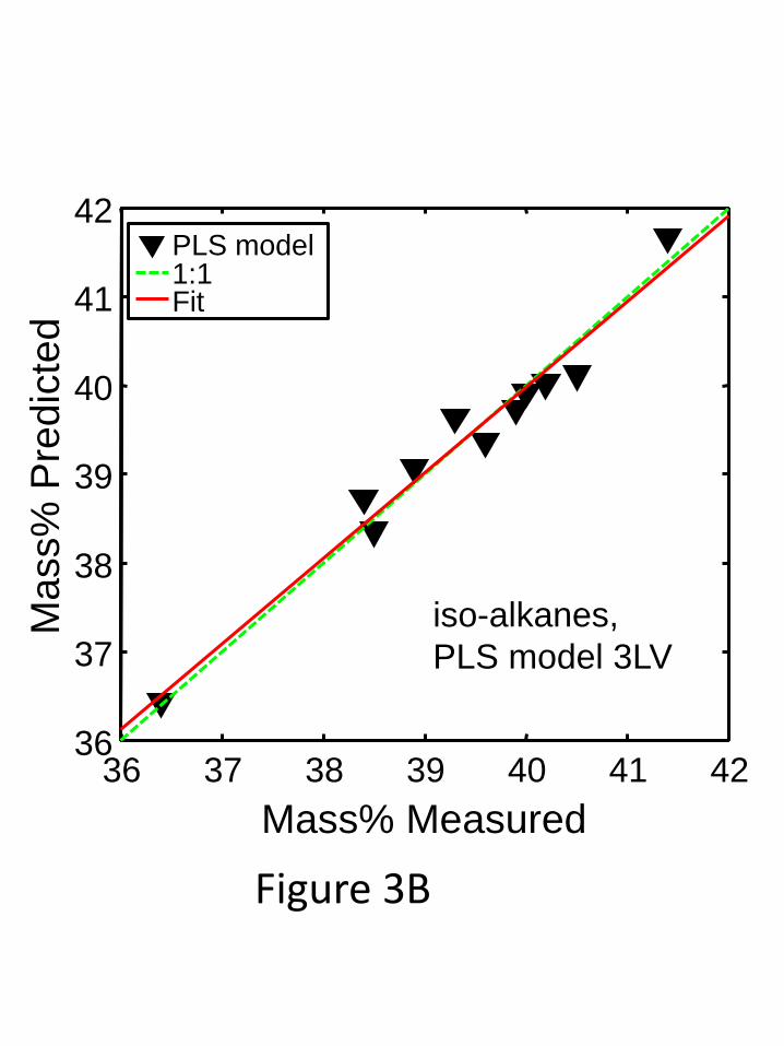
Figure 3B

36 37 38 39 40 41 42 36

37

38

39

40

41

42 PLS model 1:1 Fit

iso-alkanes,

PLS model 3LV

Mass% Measured

Ma

ss%

Pre

dic

ted

Figure 3C

26 28 30 32 34 36 38 40 26

28

30

32

34

36

38


Cycloalkanes,

PLS model 3LV

Mass% Measured

Ma

ss%

Pre

dic

ted

Figure 3D

13 14 15 16 17 18 19 13

14

15

16

17

18


Dicycloalkanes,

PLS model 3LV

Mass% Measured

Ma

ss%

Pre

dic

ted

Figure 3E

3.6 4 4.4 4.8

3.6

4

4.4

4.8 PLS model 1:1 Fit

Tricycloalkanes,

PLS model 3LV

Mass% Measured

Mass%

Pre

dic

ted

Figure 3F

0.5 1.5 2.5 3.5

0.5

1.5

2.5

3.5

Aromatics,

PLS model 3LV

PLS model 1:1 Fit

Mass% Measured

Mass%

Pre

dic

ted

Figure 4A

14.2 14.3 14.4 14.5

14.2

14.3

14.4

14.5

Hydrogen content,

PLS model 3LV

PLS model 1:1 Fit

wt% Measured

wt%

Pre

dic

ted

Figure 4B

TIC LRV Hydrogen Content

(positive)

alkanes



Tim

e,

Colu

mn 2

(se

co

nd

s)

5 10 15 20 25 30 35

0.5

1

1.5

2

2.5

cycloalkanes


Figure 4C

TIC LRV Hydrogen Content

(negative)

alkanes



Tim

e,

Colu

mn 2

(se

co

nd

s)

5 10 15 20 25 30 35

0.5

1

1.5

2

2.5

cycloalkanes


Figure 5A

804 806 808 810 812 814 816 804

806

808

810

812

814

816

Density,

PLS model 3LV

PLS model 1:1 Fit

g/l Measured

g/l P

redic

ted

Figure 5B

TIC LRV Density (positive)

alkanes



Tim

e,

Colu

mn 2

(se

co

nd

s)

5 10 15 20 25 30 35

0.5

1

1.5

2

2.5

cycloalkanes


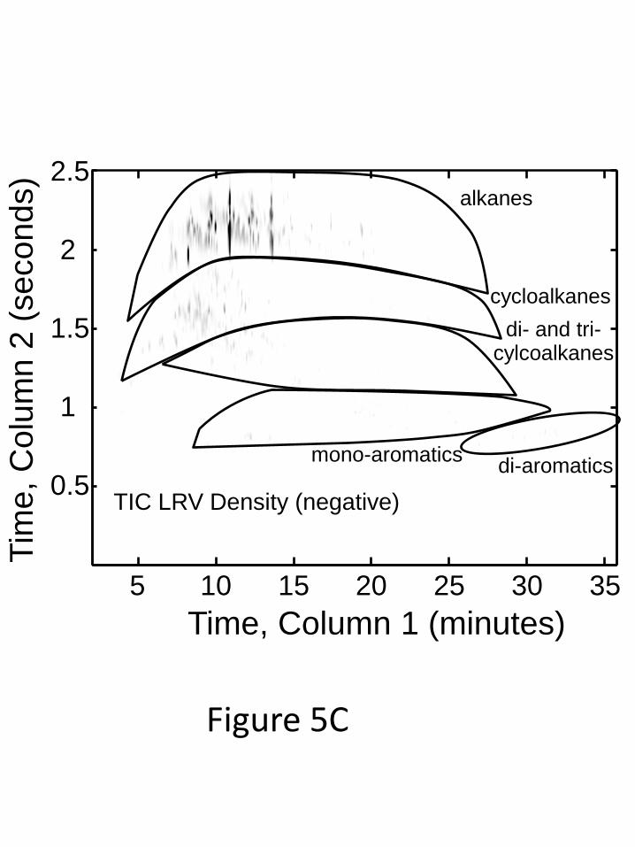
Figure 5C

TIC LRV Density (negative)

alkanes



Tim

e,

Colu

mn 2

(se

co

nd

s)

5 10 15 20 25 30 35

0.5

1

1.5

2

2.5

cycloalkanes


Figure 6A

4.6 4.8 5 5.2

4.6

4.8

5

5.2

Kinematic viscosity,

PLS model 3LV

PLS model 1:1 Fit

mm2/s Measured

mm

2/s

Pre

dic

ted

Figure 6B

TIC LRV Kinematic Viscosity

(positive)

alkanes



Tim

e,

Colu

mn 2

(se

co

nd

s)

5 10 15 20 25 30 35

0.5

1

1.5

2

2.5

cycloalkanes


Figure 6C

TIC LRV Kinematic Viscosity

(negative)

alkanes



Tim

e,

Colu

mn 2

(se

co

nd

s)

5 10 15 20 25 30 35

0.5

1

1.5

2

2.5

cycloalkanes


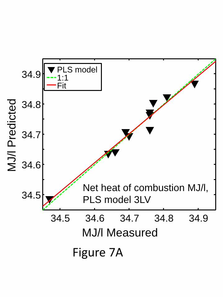
Figure 7A

34.5 34.6 34.7 34.8 34.9

34.5

34.6

34.7

34.8

34.9

Net heat of combustion MJ/l,

PLS model 3LV

PLS model 1:1 Fit

MJ/l Measured

MJ/l P

red

icte

d

Figure 7B

TIC LRV Net Heat of Combustion

(MJ/l) (positive)

alkanes



Tim

e,

Colu

mn 2

(se

co

nd

s)

5 10 15 20 25 30 35

0.5

1

1.5

2

2.5

cycloalkanes


Figure 7C

TIC LRV Net Heat of Combustion

(MJ/l) (negative)

alkanes



Tim

e,

Colu

mn 2

(se

co

nd

s)

5 10 15 20 25 30 35

0.5

1

1.5

2

2.5

cycloalkanes


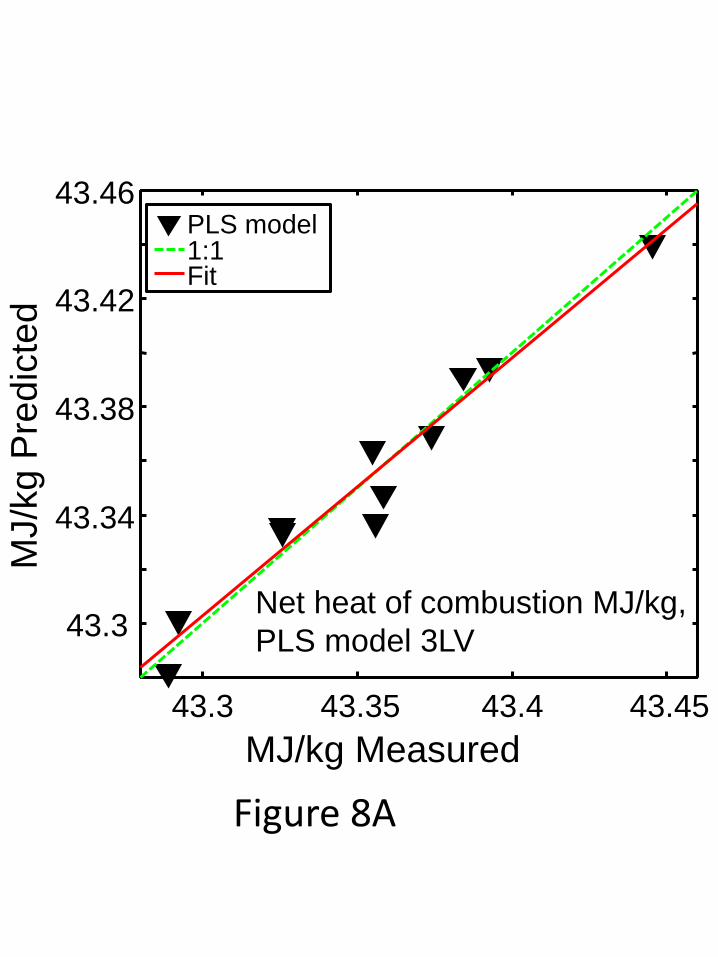
Figure 8A

43.3 43.35 43.4 43.45

43.3

43.34

43.38

43.42

43.46

Net heat of combustion MJ/kg,

PLS model 3LV

PLS model 1:1 Fit

MJ/kg Measured

MJ/k

g P

redic

ted

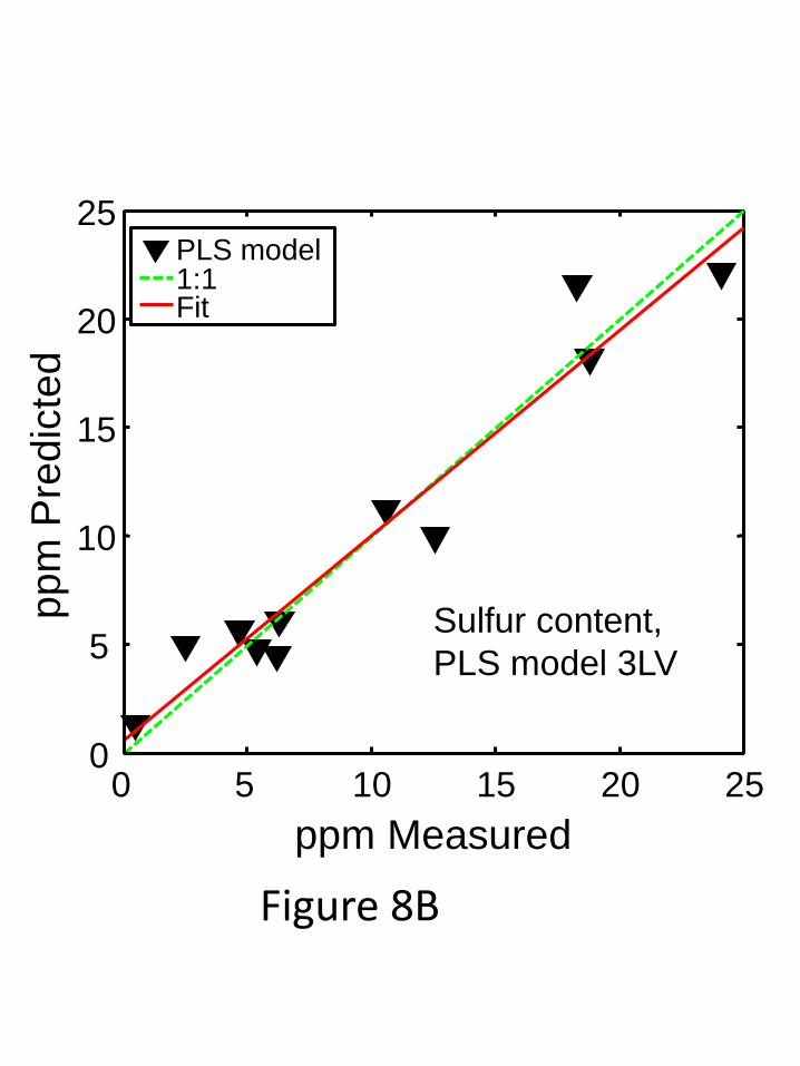
Figure 8B

0 5 10 15 20 25 0

5

10

15

20

25

Sulfur content,

PLS model 3LV

PLS model 1:1 Fit

ppm Measured

pp

m P

red

icte

d

Figure 8C

205 207 209 211 213

205

207

209

211

213

°C Measured

°C P

red

icte

d

Sustained boiling,

PLS model 3LV

PLS model 1:1 Fit

Figure 8D

207 209 211 213

207

209

211

213

215

Vapor rise,

PLS model 3LV

PLS model 1:1 Fit

°C Measured

°C P

red

icte

d

Figure 9A

iso-alkanes,

PLS model 3LV

Mass% Measured

Mass%

Pre

dic

ted

37 39 41

37

39

41

Validation 1:1

Figure 9B

Tricycloalkanes,

PLS model 3LV

Mass% Measured

Ma

ss%

Pre

dic

ted

3.6 4 4.4 4.8

3.6

4

4.4

4.8 Validation 1:1

Figure 9C

wt% Measured

wt%

Pre

dic

ted

14.2 14.3 14.4 14.5

14.2

14.3

14.4

14.5

Hydrogen content,

PLS model 3LV

Validation 1:1

Figure 9D

g/l Measured

g/l P

red

icte

d

806 810 814

806

810

814

Density,

PLS model 3LV

Validation 1:1

1. report date 2. report type journal article · report documentation page ... correlation of rp-1...

Documents