1

RecapRecap

2

Complex Instruction Set Computing(CISC)

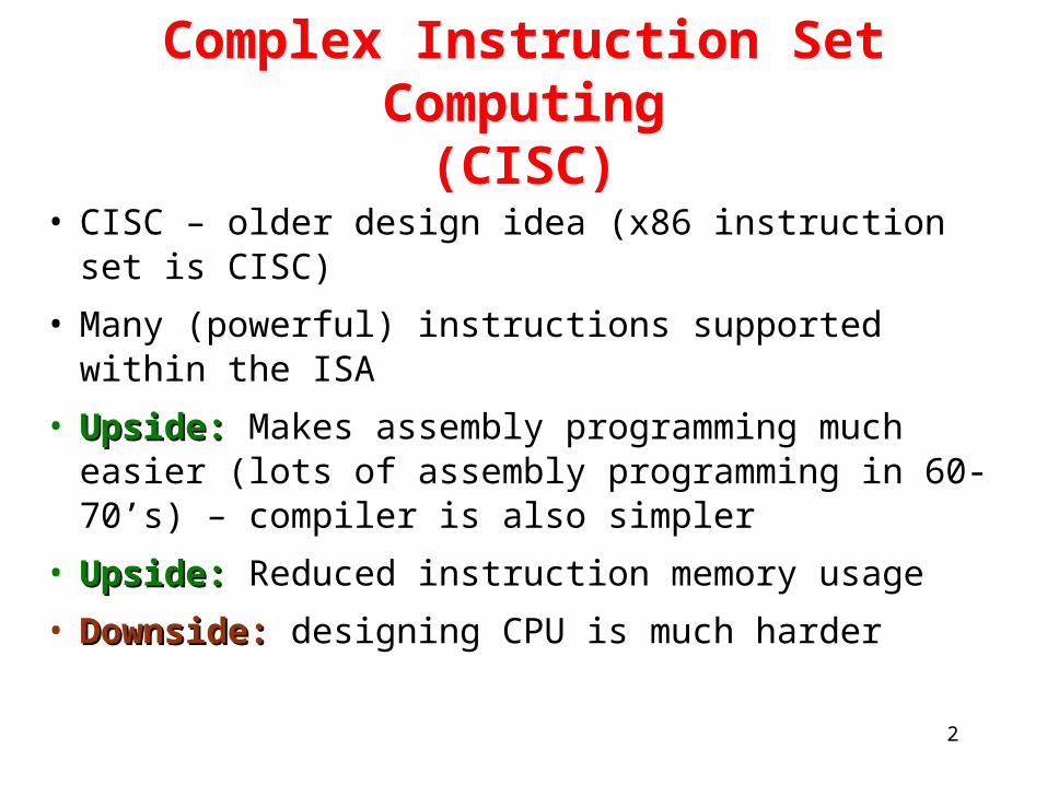
• CISC – older design idea (x86 instruction set is CISC)

• Many (powerful) instructions supported within the ISA

• Upside:Upside: Makes assembly programming much easier (lots of assembly programming in 60-70’s) – compiler is also simpler

• Upside:Upside: Reduced instruction memory usage

• Downside:Downside: designing CPU is much harder

3

Reduced Instruction Set Computing(CISC)

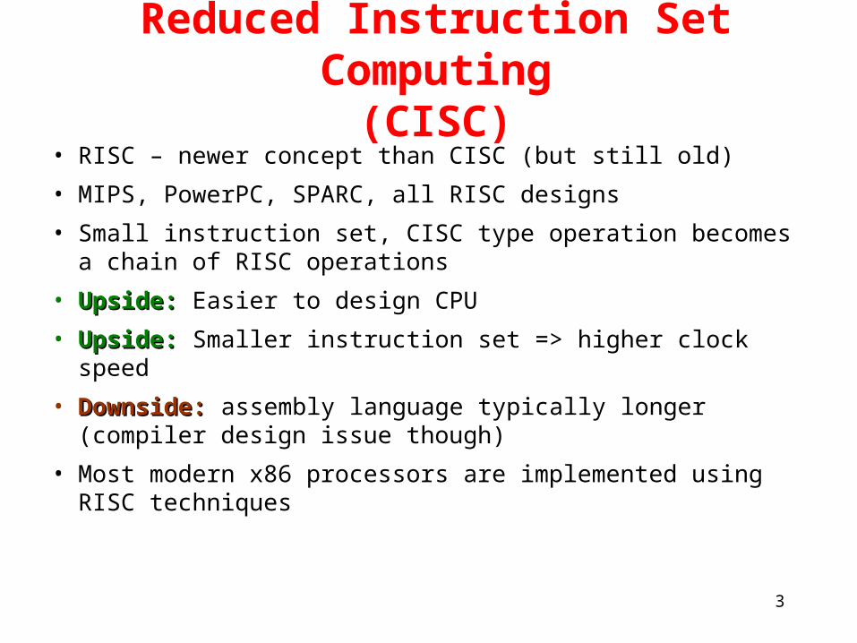
• RISC – newer concept than CISC (but still old)

• MIPS, PowerPC, SPARC, all RISC designs

• Small instruction set, CISC type operation becomes a chain of RISC operations

• Upside:Upside: Easier to design CPU

• Upside:Upside: Smaller instruction set => higher clock speed

• Downside:Downside: assembly language typically longer (compiler design issue though)

• Most modern x86 processors are implemented using RISC techniques

4

Birth of RISC

• Roots can be traced to two research projects– Berkeley RISC processor (~1980, D. Patterson)

– Stanford MIPS processor (~1981, J. Hennessy)

• Stanford & Berkeley projects driven by interest in building a simple chip that could be made in a university environment

• Commercialization benefited from these two independent projects– Berkeley Project -> began Sun Microsystems

– Stanford Project -> began MIPS (used by SGI)

5

Who “won”?

• Modern x86 are RISC-CISC hybrids– ISA is translated at hardware level to shorter instructions

– Very complicated designs though, lots of scheduling scheduling hardwarehardware

• MIPS, Sun SPARC, DEC Alpha are much truer implementations of the RISC ideal

• Modern metric for determining RISCkyness of design: does the ISA have LOAD STORE instructions to memory?

6

Modern RISC processors

• Complexity has nonetheless increased significantly

• Superscalar execution (where CPU has multiple functional units of the same type e.g. two add units) require complex circuitry to control scheduling of operations

• What if we could remove the scheduling complexity by using a smart compilersmart compiler…?

7

VLIW & EPIC• VLIW – very long instruction word

• Idea: pack a number of non- interdependent operations into one long instruction

• Strong emphasis on compilers to schedule instructions

• Natural successor to RISC – designed to avoid the need for complex scheduling in RISC designs

• ISA is called IA-64

Instr 1

Instr 2

Instr 3

3 instructions scheduledinto one long instruction word

8

The EPIC Philosophy

9

Bundle Templates

• Not all combinations of A, I, M, F, B, L and X are permitted

• Group “stops” are explicitly encoded as part of the template– can’t stop just anywhere

Some bundles identicalexcept for group stop

10

Individual Instruction Formats• Fairly RISC-like like

– easy to decode, fields tend to stay put

11

Instruction Format: Bundles & Templates

•Bundle•Set of three instructions (41 bits each)

•Template •Identifies types of instructions in bundle

12

MEM MEM INT INT FP FP B B B

128-bit instruction bundles from I-cacheS2 S1 S0 T

Fetch one or more bundles for execution(Implementation, Itanium® takes two.)

Try to execute all instructions inparallel, depending on available units.

Retired instruction bundles

Processor

Explicitly Parallel Instruction ComputingEPIC

functional units

MEM MEM INT INT FP FP B B B

13

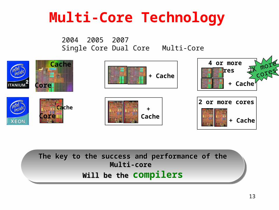
Multi-Core Technology

2004 2005 2007 Single Core Dual Core Multi-Core

+ Cache

+ Cache

Cache

Core

4 or more cores

+ Cache

CoreCache

2 or more cores

+ Cache

2X more

cores

The key to the success and performance of the Multi-core The key to the success and performance of the Multi-core

Will be the Will be the compilersThe key to the success and performance of the Multi-core The key to the success and performance of the Multi-core

Will be the Will be the compilers

14

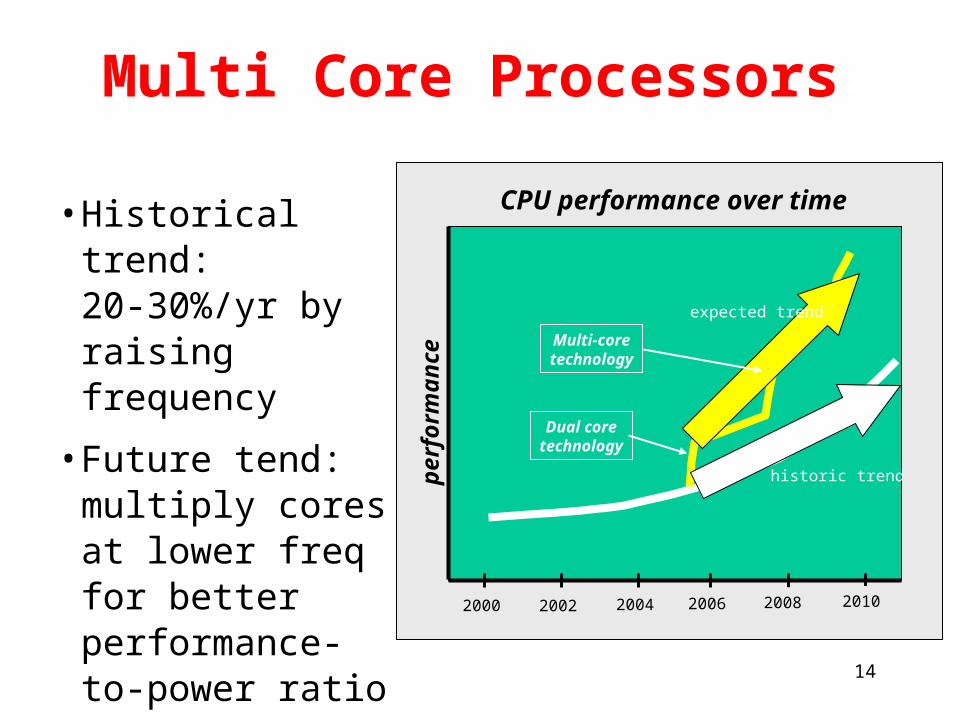
Multi Core Processors

• Historical trend: 20-30%/yr by raising frequency

• Future tend: multiply cores at lower freq for better performance-to-power ratio

2000

perf

orm

an

ce

CPU performance over time

historic trend

expected trend

Dual coretechnology

Multi-coretechnology

2002

2004

2006

2008

2010

15

64-Bit 64-Bit ProcessorsProcessors

16

32-bit Computing

• In computer architecture, a wordword is defined as a unit of data that can be addressed and moved between the computer processor and the storage area.

• In 32-bit computing a word is 32 bits.

• Usually, the defined bit-length of a word is equivalent to the width of the computer's data busdata bus (and registersregisters) so that a word can be moved in a single operation from the storage to the processor registers

17

32-bit Computing

• In a 32-bit microprocessor;

– There are 32-bit general purpose registers in the processor.

– There are 232 = 4GB memory to be addressed.

18

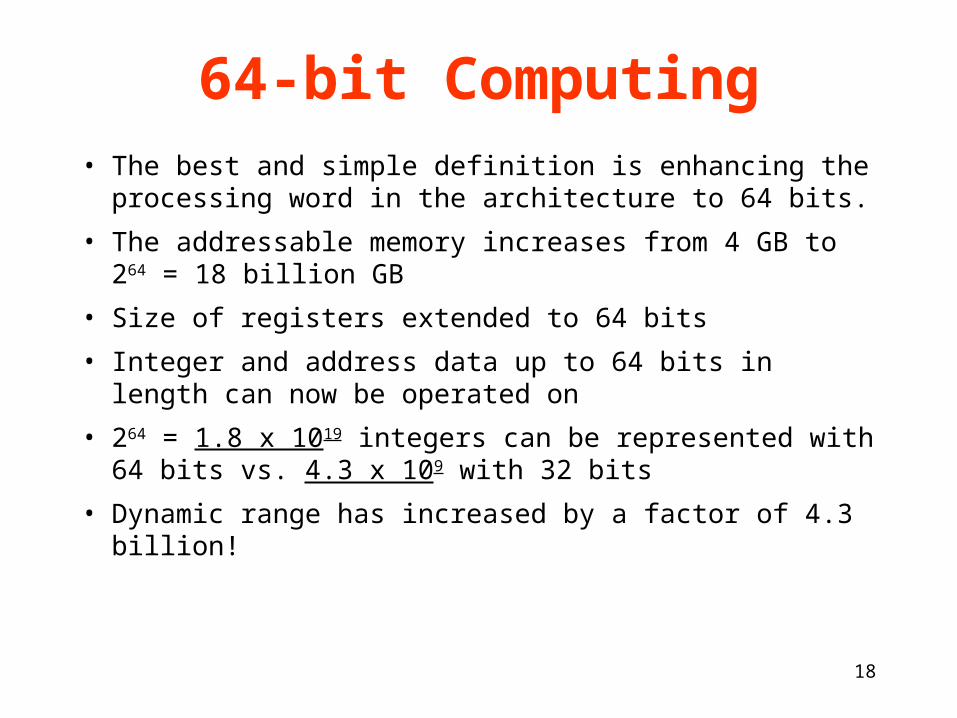
64-bit Computing• The best and simple definition is enhancing the processing

word in the architecture to 64 bits.

• The addressable memory increases from 4 GB to 264 = 18 billion GB

• Size of registers extended to 64 bits

• Integer and address data up to 64 bits in length can now be operated on

• 264 = 1.8 x 1019 integers can be represented with 64 bits vs. 4.3 x 109 with 32 bits

• Dynamic range has increased by a factor of 4.3 billion!

19

64-bit Processor Basics• Stepping up from 32

to 64 bits does not mean doubling performance

• Certain applications will benefit, others will not

20

What Applications Can Benefit Most From 64-bit?

• Large databases

• Business and scientific simulation and modeling programs

• Highly graphics-intensive software (CAD, 3-D games)

• Cryptography

• Etc.

21

Benefits of 64-bit Computing

• Allowing applications to store vast amounts of data in main memory.

• Allowing complex calculations with a high-level precision.

• Manipulating data and executing instructions in chunks that are twice as large as in 32-bit computing.

22

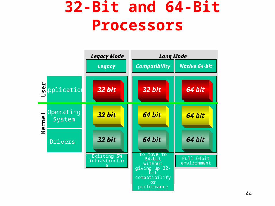
32-Bit and 64-Bit Processors

Use

rK

ern

el

Application

OperatingSystem

Drivers

Full 64bit environment

64 bit

64 bit

64 bit

Native 64-bit

Allows users to move to 64-bit without giving

up 32-bit compatibility or

performance

64 bit

64 bit

32 bit

Compatibility

Existing SW infrastructure

32 bit

32 bit

32 bit

Legacy

Long ModeLegacy Mode

23

The Role of The Role of CompilersCompilers

24

Compiler and ISA

• Almost all programming is done in high-level language (HLL) for desktop and server applications

• Most instructions executed are the output of a compiler

• So, separation from each other is impractical

25

Goal of the Compiler

• Primary goal is correctness

• Second goal is speed of the object code

• Others:– Speed of the compilation– Ease of providing debug support– Inter-operability among languages

26

Typical Modern Compiler Structure

Common Intermediate Representation

Somewhat language dependentLargely machine independent

Small language dependentSlight machine dependent

Language independentHighly machine dependent

27

Optimization Types• High level - done at source code level

– Procedure called only once - so put it in-line and save CALL

• Local - done on basic sequential block (straight-line code)– Common sub-expressions produce same value

– Constant propagation - replace constant valued variable with the constant - saves multiple variable accesses with same value

• Global - same as local but done across branches– Code motion - remove code from loops that compute same value

on each pass and put it before the loop

28

Optimization Types (Cont.)• Register allocation

– Use graph coloring (graph theory) to allocate registers• NP-complete

• Heuristic algorithm works best when there are at least 16 (and preferably more) registers

• Processor-dependent optimization– Strength reduction: replace multiply with shift and add sequence

– Pipeline scheduling: reorder instructions to minimize pipeline stalls

– Branch offset optimization: Reorder code to minimize branch offsets

29

Constant propagation

a:= 5; ...// no change to a so far.if (a > b) { . . . }

The statement (a > b) can be replaced by (5 > b). This could free a register when the comparison is executed.

When applied systematically, constant propagation can improve the code significantly.

30

Strength reduction

Example:

for (j = 0; j = n; ++j) A[j] = 2*j;

for (i = 0; 4*i <= n; ++i) A[4*i] = 0;

An optimizing compiler can replace multiplication by 4 by addition by 4.

This is an example of strength reduction.In general, scalar multiplications can be replaced by additions.

31

Major Types of Optimizations and Example in Each Class

Optimization Name Explanation % of the total number of optimizing

transformations

High Level At or near the source level; machine-independent

Not Measured

Local Within Straight Line Code 40%

Global Across a Branch 42%

Machine Dependent Depends on Machine Knowledge Not Measured

32

MIPS: Case Study of

Instruction Set Architecture

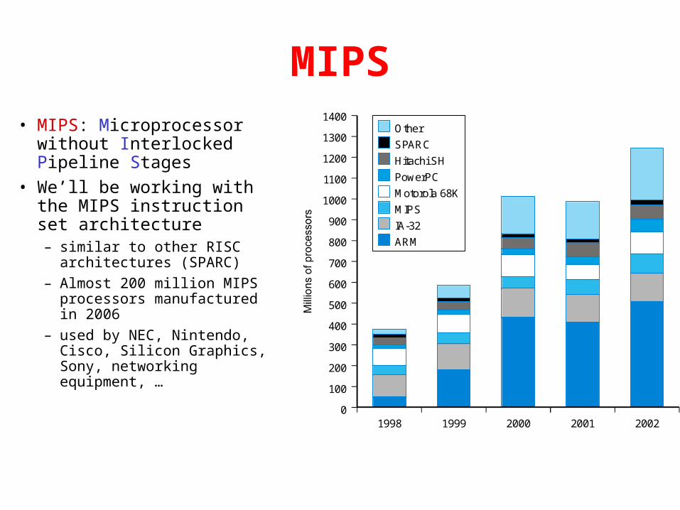
MIPS• MIPS: Microprocessor without

Interlocked Pipeline Stages

• We’ll be working with the MIPS instruction set architecture– similar to other RISC

architectures (SPARC)

– Almost 200 million MIPS processors manufactured in 2006

– used by NEC, Nintendo, Cisco, Silicon Graphics, Sony, networking equipment, …

1400

1300

1200

1100

1000

900

800

700

600

500

400

300

200

100

01998 2000 2001 20021999

Other

SPARC

Hitachi SH

PowerPC

Motorola 68K

MIPS

IA-32

ARM

34

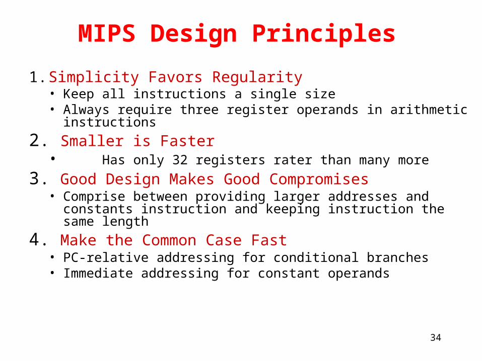
MIPS Design Principles

1. Simplicity Favors Regularity• Keep all instructions a single size• Always require three register operands in arithmetic instructions

2. Smaller is Faster• Has only 32 registers rater than many more

3. Good Design Makes Good Compromises• Comprise between providing larger addresses and constants

instruction and keeping instruction the same length

4. Make the Common Case Fast• PC-relative addressing for conditional branches• Immediate addressing for constant operands

35

MIPS Registers and Memory

Memory4GB Max

(Typically 64MB-1GB)

0x000000000x000000040x000000080x0000000C0x000000100x000000140x000000180x0000001C

0xfffffff40xfffffffc

0xfffffffc

PC = 0x0000001C

Registers

32 General Purpose Registers

R0R1R2

R30R31

32 bits

–232 bytes with addresses 0, 1, 2, …, 232-1

36

MIPS Registers and Usage

Name Register number Usage$zero 0 the constant value 0$at 1 reserved for assembler$v0-$v1 2-3 values for results and expression evaluation$a0-$a3 4-7 arguments$t0-$t7 8-15 temporary registers$s0-$s7 16-23 saved registers$t8-$t9 24-25 more temporary registers$k0-$k1 26-27 reserved for Operating System kernel$gp 28 global pointer$sp 29 stack pointer$fp 30 frame pointer$ra 31 return address

Each register can be referred to by number or name.

37

MIPS Instructions

• All instructions exactly 32 bits wide• Different formats for different purposes• Similarities in formats ease implementation

op rs rt offset

6 bits 5 bits 5 bits 16 bits

op rs rt rd functshamt

6 bits 5 bits 5 bits 5 bits 5 bits 6 bits

R-Format

I-Format

op address

6 bits 26 bits

J-Format

31 0

31 0

31 0

38

MIPS Instruction Types

• Arithmetic & Logical - manipulate data in registersadd $s1, $s2, $s3 $s1 = $s2 + $s3or $s3, $s4, $s5 $s3 = $s4 OR $s5

• Data Transfer - move register data to/from memorylw $s1, 100($s2) $s1 = Memory[$s2 + 100]sw $s1, 100($s2) Memory[$s2 + 100] = $s1

• Branch - alter program flowbeq $s1, $s2, 25 if ($s1==$s1) PC = PC + 4 + 4*25

39

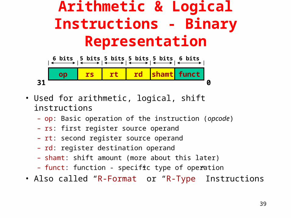
Arithmetic & Logical Instructions - Binary Representation

• Used for arithmetic, logical, shift instructions– op: Basic operation of the instruction (opcode)

– rs: first register source operand

– rt: second register source operand

– rd: register destination operand

– shamt: shift amount (more about this later)

– funct: function - specific type of operation

• Also called “R-Format” or “R-Type” Instructions

op rs rt rd functshamt

6 bits 5 bits 5 bits 5 bits 5 bits 6 bits

031

40

op rs rt rd functshamt

6 bits 5 bits 5 bits 5 bits 5 bits 6 bits

Decimal

Binary

Arithmetic & Logical Instructions -Binary Representation Example

• Machine language for add $8, $17, $18

• op, funct values already defined

000000

0

10001

17

10010

18

01000

8

00000

0

100000

32

031

41

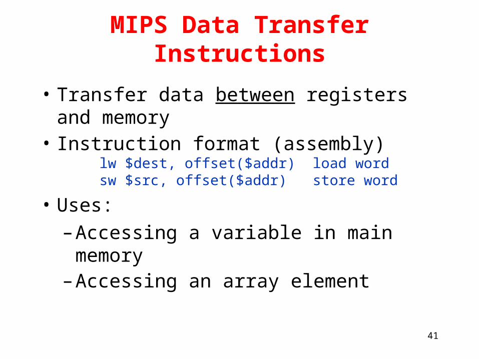
MIPS Data Transfer Instructions

• Transfer data between registers and memory

• Instruction format (assembly)lw $dest, offset($addr) load wordsw $src, offset($addr) store word

• Uses:

– Accessing a variable in main memory– Accessing an array element

42

Example - Loading a Simple Variable

lw R5,8(R2) Memory

0x00

Variable Z = 692310

Variable XVariable Y

0x040x080x0c0x100x140x180x1c

8

+

Registers

R0=0 (constant)R1

R2=0x10

R30R31

R3R4R5R5

R2=0x10

R5 = 629310Variable Z = 692310

43

Data Transfer Instructions - Binary Representation

• Used for load, store instructions– op: Basic operation of the instruction (opcode)

– rs: first register source operand

– rt: second register source operand

– offset: 16-bit signed address offset (-32,768 to +32,767)

• Also called “I-Format” or “I-Type” instructions

op rs rt offset

6 bits 5 bits 5 bits 16 bits

Address

44

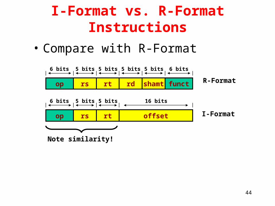
I-Format vs. R-Format Instructions

• Compare with R-Format

offset

6 bits 5 bits 5 bits 16 bits

I-Formatop rs rt

rd functshamt

6 bits 5 bits 5 bits 5 bits 5 bits 6 bits

R-Formatop rs rt

Note similarity!

45

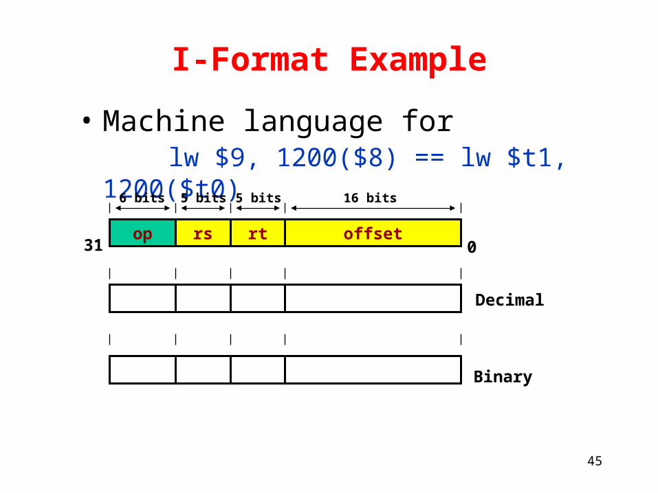
I-Format Example

• Machine language for lw $9, 1200($8) == lw $t1, 1200($t0)

op rs rt offset

6 bits 5 bits 5 bits 16 bits

Binary

Decimal35 8 9 1200

100011 01000 01001 0000010010110000

031

46

MIPS Conditional Branch Instructions

• Conditional branches allow decision makingbeq R1, R2, LABEL if R1==R2 goto LABELbne R3, R4, LABEL if R3!=R4 goto LABEL

ExampleC Code if (i==j) goto L1;

f = g + h; L1: f = f - i;

Assembly beq $s3, $s4, L1add $s0, $s1, $s2

L1: sub $s0, $s0, $s3

47

Binary Representation - Branch

• Branch instructions use I-Format• offset is added to PC when branch is taken

beq r0, r1, offset

has the effect:

if (r0==r1) pc = pc + 4 + offset else pc = pc + 4;

op rs rt offset

6 bits 5 bits 5 bits 16 bits

48

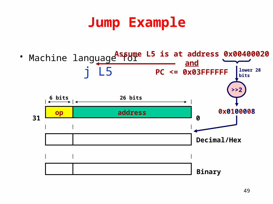
Binary Representation - Jump

• Jump Instruction uses J-Format (op=2)• What happens during execution?

PC = PC[31:28] : (IR[25:0] << 2)

op address

6 bits 26 bits

Conversion to word offset

Concatenate upper 4 bits of PC to form complete32-bit address

49

Jump Example

• Machine language for j L5

Assume L5 is at address 0x00400020and

PC <= 0x03FFFFFF

Binary

Decimal/Hex

op address

6 bits 26 bits

2 0x0100008

000010 00000100000000000000001000

>>2

lower 28bits

0x010000831 0

50

Summary: MIPS InstructionsMIPS assembly language

Category Instruction Example Meaning Commentsadd add $s1, $s2, $s3 $s1 = $s2 + $s3 Three operands; data in registers

Arithmetic subtract sub $s1, $s2, $s3 $s1 = $s2 - $s3 Three operands; data in registers

add immediate addi $s1, $s2, 100 $s1 = $s2 + 100 Used to add constants

load w ord lw $s1, 100($s2) $s1 = Memory[$s2 + 100]Word from memory to register

store w ord sw $s1, 100($s2) Memory[$s2 + 100] = $s1 Word from register to memory

Data transfer load byte lb $s1, 100($s2) $s1 = Memory[$s2 + 100]Byte from memory to register

store byte sb $s1, 100($s2) Memory[$s2 + 100] = $s1 Byte from register to memoryload upper immediate

lui $s1, 100 $s1 = 100 * 216 Loads constant in upper 16 bits

branch on equal beq $s1, $s2, 25 if ($s1 == $s2) go to PC + 4 + 100

Equal test; PC-relative branch

Conditional

branch on not equal bne $s1, $s2, 25 if ($s1 != $s2) go to PC + 4 + 100

Not equal test; PC-relative

branch set on less than slt $s1, $s2, $s3 if ($s2 < $s3) $s1 = 1; else $s1 = 0

Compare less than; for beq, bne

set less than immediate

slti $s1, $s2, 100 if ($s2 < 100) $s1 = 1; else $s1 = 0

Compare less than constant

jump j 2500 go to 10000 Jump to target address

Uncondi- jump register jr $ra go to $ra For sw itch, procedure return

tional jump jump and link jal 2500 $ra = PC + 4; go to 10000 For procedure call

51

Byte Halfword Word

Registers

Memory

Memory

Word

Memory

Word

Register

Register

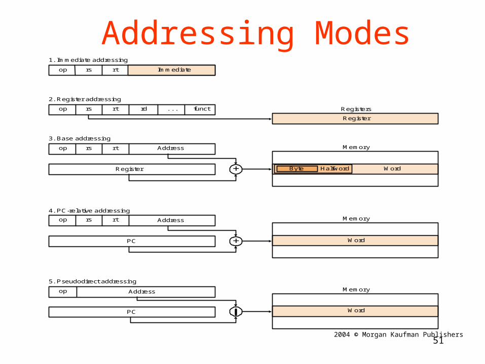
1. Immediate addressing

2. Register addressing

3. Base addressing

4. PC-relative addressing

5. Pseudodirect addressing

op rs rt

op rs rt

op rs rt

op

op

rs rt

Address

Address

Address

rd . . . funct

Immediate

PC

PC

+

+

2004 © Morgan Kaufman Publishers

Addressing Modes

52

Summary - MIPS Instruction Set

• simple instructions all 32 bits wide• very structured, no unnecessary baggage

• only three instruction formats

op rs rt offset

6 bits 5 bits 5 bits 16 bits

op rs rt rd functshamt

6 bits 5 bits 5 bits 5 bits 5 bits 6 bits

R-Format

I-Format

op address

6 bits 26 bits

J-Format