1 real-world evolution of the yield curve riccardo rebonato sukhdeep mahal royal bank of scotland -...
TRANSCRIPT
1
Real-World Evolution of the Yield Curve
Riccardo Rebonato
Sukhdeep Mahal
Royal Bank of Scotland - QUARC
Geneva 2002
2
The problem
• There exist a very large number of models that produce the evolution of the yield curve under a variety of assumptions.
• Examples :– One-factor short-rate models (BDT, BK, HW)– HJM/BGM– Multi-factor short-rate models (LS, HW, RR)– etc.
3
Why do we need another one?
• All these models produce the evolution of the yield curve in the risk-adjusted measure, not in the real-world measure. For risk management purposes I need to evolve the yield curve in the real measure (and, contingent on the future state of the world having been attained, to value instruments in the risk-adjusted measure).

4
Does it really make a difference?
• Consider the case of commodities: a forward-curve in backwardation does not reflect future real-world expectations, but the premium assigned to holding the physical commodity today.
5
Objection
• With commodities cash-and-carry arbitrage does not really work. Perhaps everything is fine with forward rates.
• Consider the LMM. The forward rates display a drift upward or downwards depending on the (arbitrary) choice of numeraire. Imagine the effect after 10 years.

6
Why is there a difference between the two measures?
• The forward rates contain an expectation component and a risk premium.
• Heath (HJM): ‘The forward rates have nothing to do with expectation of future rates’. A bit too strong.
• At very short horizons, it would take an extremely risk-averse utility function to drive an appreciable wedge between expectations in different measures. Over long horizons, the differences can become very large.

7
Why do I need to evolve the yield curve?
• Typical market risk (trading book) applications require to evolve the yield curve over very small steps (1 day, 10 days).
• The risk premium is not a big issue.
• For other risk-management applications the time horizon can be orders of magnitude longer.
8
What are these applications?
• Counterparty credit risk exposure
• Analysis of effectiveness of hedging/trading strategies
• A/L (balance sheet) management
• Performance analysis and asset allocation choice for investment portfolios
9
The methodology
• Constructing a series of IR paths
The goal is to produce future IR paths that incorporate as accurately as possible the information from historical correlated moves of yield curves, collected over a long period of times.

10
Do we need accurate paths?
These simulations must be accurate because they will be used
to make comparison between different asset classes to gauge risk/reward profiles to establish reasonable bands of variation for the NII To test hedging strategies under realistic scenarios
(not just the usual rigid shifts up and down of the yield curve)
11
The usual solution
• Do a PCA of the (relative) changes
• Retain m eigenvectors
• Rescale the eigenvalues
• Evolve the yield curve by drawing iid random draws (one for each factor and time step)
12
Observation 1
• The procedure is valid only if the underlying joint process is a diffusion. I can always orthogonalize a covariance matrix, and work with the eigen-vectors/values, but I will only get back the original process if the original process was a joint diffusion with iid increments to start with.

13
Observation 2
• By drawing iid random draws that are independent both across factors and serially one is making a very strong assumption about the homoskedaticity and the lack of serial dependence in the data
• I shall show that these assumptions are strongly unwarranted

14
A naïve approach (totally non-parametric)
• Collect a large number of synchronous changes in yields, labelled by an index i, i=1,2,…,n.
• Draw a uniform variate from U[0,1]
• Map the variate to an integer between 1 and n, say, k
• Apply the k-th vector of rate changes to the current yield curve
• Continue

15
CommentThe approach might be simple, but it is by
construction guaranteed to recover as best as possible given the sample size:
• all the correct PC (eigenvectors and eigenvalues)
• all the correct unconditional marginal distributions for all the yields (all moments).
Not every method can deliver this!

16
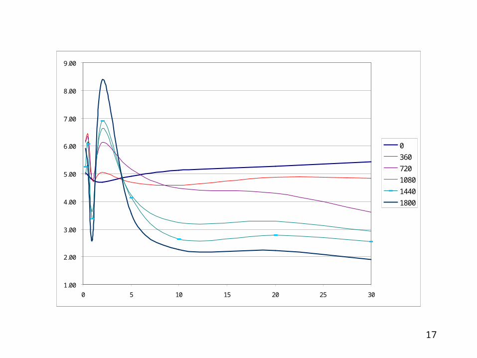
Unfortunately it is not good enough!
3.00
5.00
7.00
9.00
11.00
13.00
15.00
0 5 10 15 20 25 30
0
360
720
1080
1440
1800
17
1.00
2.00
3.00
4.00
5.00
6.00
7.00
8.00
9.00
0 5 10 15 20 25 30
0
360
720
1080
1440
1800

18
2.00
3.00
4.00
5.00
6.00
7.00
8.00
9.00
10.00
11.00
12.00
0 5 10 15 20 25 30
0
360
720
1080
1440
1800

19
3.00
4.00
5.00
6.00
7.00
8.00
9.00
10.00
11.00
12.00
13.00
0 5 10 15 20 25 30
0
360
720
1080
1440
1800

20
Real yield curves just do not look like this!
• How can we quantify this lack of ‘plausibility’?
• The origin is clearly in the curvature: in real life we observe sharp changes in slope at the very short end, but not as pronounced for longer maturities.

21
Let’s look at the distribution of curvatures
-500
0
500
1000
1500
2000
-0.5 -0.3 -0.1 0.1 0.3 0.5
Freq6m
Freq1y
Freq2y
Freq5y
Frequency

22
Freq6m
-50
0
50
100
150
200
250
300
350
-1 -0.5 0 0.5 1
Freq6m

23
Freq1y
-50
0
50
100
150
200
250
300
350
400
-0.5 -0.3 -0.1 0.1 0.3 0.5
Freq1y

24
-100
0
100
200
300
400
500
600
-0.5 -0.3 -0.1 0.1 0.3 0.5
Freq1y
Freq2y

25
-200
0
200
400
600
800
1000
1200
1400
1600
1800
-0.5 -0.3 -0.1 0.1 0.3 0.5
Freq1y
Freq5y

26
Density of curvatures: DEPOSIT_USD_3M to DEPOSIT_USD_1Y
0.00
0.02
0.04
0.06
0.08
0.10
0.12
0.14
0.16
0.18
0.20
-0.06 -0.04 -0.02 0.00 0.02 0.04 0.06

27
Density of curvatures: DEPOSIT_USD_6M to BOND_USD_2Y
0.00
0.01
0.02
0.03
0.04
0.05
0.06
0.07
0.08
-0.01 0.00 0.01 0.02 0.03 0.04 0.05 0.06

28
Density of curvatures: BOND_USD_5Y to BOND_USD_20Y
0.00
0.01
0.02
0.03
0.04
0.05
0.06
0.07
0.08
0.09
-0.0
002
-0.0
001
0.00
00
0.00
01
0.00
02
0.00
03
0.00
04
0.00
05
0.00
06
0.00
07
0.00
08
29
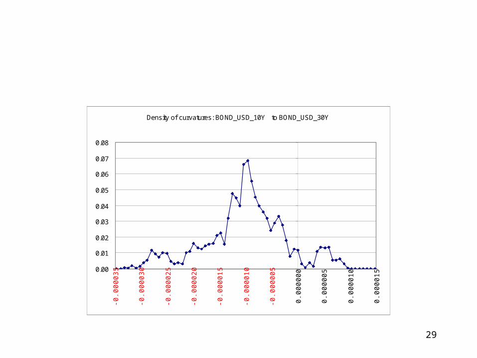
Density of curvatures: BOND_USD_10Y to BOND_USD_30Y
0.00
0.01
0.02
0.03
0.04
0.05
0.06
0.07
0.08
-0.0
0003
5
-0.0
0003
0
-0.0
0002
5
-0.0
0002
0
-0.0
0001
5
-0.0
0001
0
-0.0
0000
5
0.00
0000
0.00
0005
0.00
0010
0.00
0015

30
Density of changes in curvatures: DEPOSIT_USD_3M to DEPOSIT_USD_1Y
0.00
0.05
0.10
0.15
0.20
0.25
0.30
0.35
0.40
0.45
-0.0
25
-0.0
20
-0.0
15
-0.0
10
-0.0
05
0.00
0
0.00
5
0.01
0
0.01
5
0.02
0
0.02
5
31
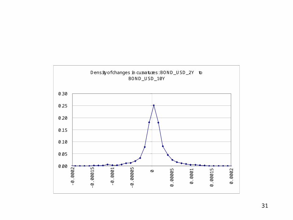
Density of changes in curvatures: BOND_USD_2Y to BOND_USD_10Y
0.00
0.05
0.10
0.15
0.20
0.25
0.30
-0.0
00
2
-0.0
00
15
-0.0
00
1
-0.0
00
05 0
0.0
00
05
0.0
00
1
0.0
00
15
0.0
00
2
32
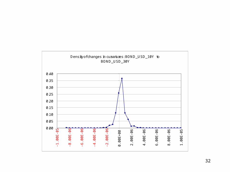
Density of changes in curvatures: BOND_USD_10Y to BOND_USD_30Y
0.00
0.05
0.10
0.15
0.20
0.25
0.30
0.35
0.40
-1.0
0E
-05
-8.0
0E
-06
-6.0
0E
-06
-4.0
0E
-06
-2.0
0E
-06
0.0
0E
+0
0
2.0
0E
-06
4.0
0E
-06
6.0
0E
-06
8.0
0E
-06
1.0
0E
-05

33
Comments
• At the short end the curvature can be very high, both positive and negative - short terms expectations influence the forward rates a lot
• At the longer end the distribution of curvatures is much more peaked

34
What keeps the yield curve smooth?
• Assume that, as the yield curve ‘diffuses’, small ‘kinks’ appear
• ‘Arbitrageurs’ are enticed to move in with barbell trades, receiving the high yields and paying the low one
• This automatically reduces the curvature

35
Why don’t arbitrageurs do the same at the short end?
• At the short end they are afraid that the kink in the curve might reflect expectations about rapidly changing rate expectations (V-shaped recovery of 2001)
• At the long end it is more difficult to make an expectation story around the 9-10 year area
• The longer the maturity, the fewer the kinks

36
How can we model this?
• Consider a HLH barbell: buying the high yields and selling the low yield is equivalent to introducing springs in the yield curve
• This is reflected in a drift term proportional to the local curvature
• End effects to be treated separately

37
How do we choose the spring constants?
• We can choose the different spring constants across the yield curve in such a way that the model-produced distribution of curvatures will match some features (eg second moment) of the real-world distribution of curvatures as a function of maturity
• So, at the short end the springs are very weak (large curvatures can occur).
• At the long end curvatures are strong (curve does not get kinky).

38
An added bonus
• To the extent that what has been added is a drift term, asymptotically I have not affected the covariance matrix
• Therefore the new procedure preserves all the positive features of the naïve approach
• In particular it still recovers correctly all the eigenvalues and the eigenvectors (PCA) and the unconditional marginal distributions

39
A Comment
Incidentally, this gives an idea of how weak the PCA requirement
really is!
40
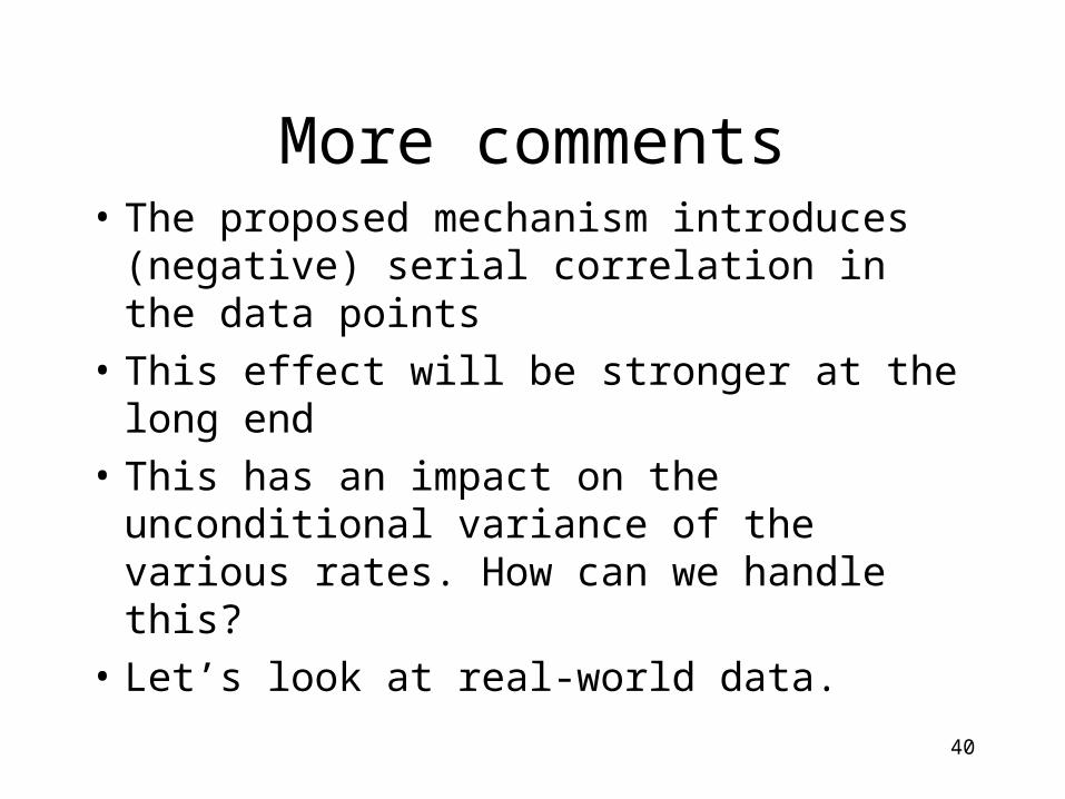
More comments• The proposed mechanism introduces
(negative) serial correlation in the data points
• This effect will be stronger at the long end
• This has an impact on the unconditional variance of the various rates. How can we handle this?
• Let’s look at real-world data.

41
Serial Variance: DEPOSIT_USD_3M
0.0000
0.0020
0.0040
0.0060
0.0080
0.0100
0.0120
1 6 11 16 21 26 31 36 41 46 51 56 61 66
n-day non-overlapping changes
42
Serial Variance: DEPOSIT_USD_6M
0.000
0.002
0.004
0.006
0.008
0.010
0.012
1 6 11 16 21 26 31 36 41 46 51 56 61 66
n-day non-overlapping changes
43
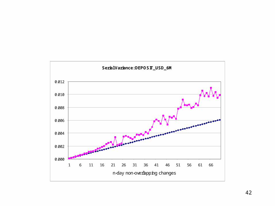
Serial Variance: DEPOSIT_USD_1Y
0.000
0.002
0.004
0.006
0.008
0.010
0.012
0.014
0.016
1 6 11 16 21 26 31 36 41 46 51 56 61 66
n-day non-overlapping changes

44
Serial Variance: BOND_USD_2Y
0.000
0.002
0.004
0.006
0.008
0.010
0.012
0.014
0.016
1 6 11 16 21 26 31 36 41 46 51 56 61 66
n-day non-overlapping changes
45
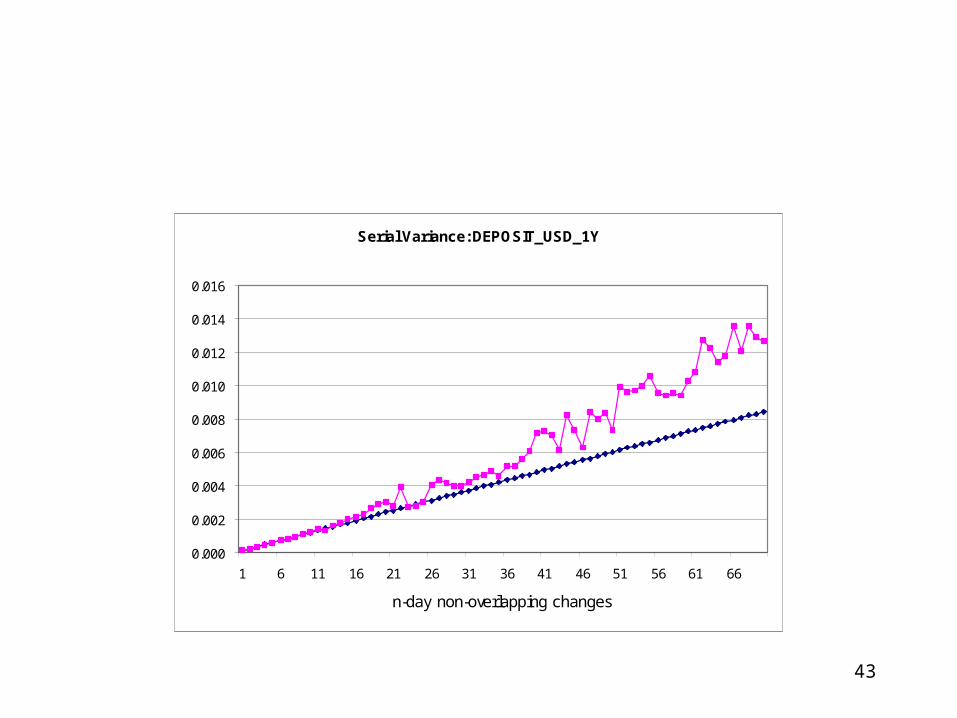
Serial Variance: BOND_USD_10Y
0.000
0.001
0.002
0.003
0.004
0.005
0.006
0.007
0.008
0.009
1 6 11 16 21 26 31 36 41 46 51 56 61 66
n-day non-overlapping changes
46
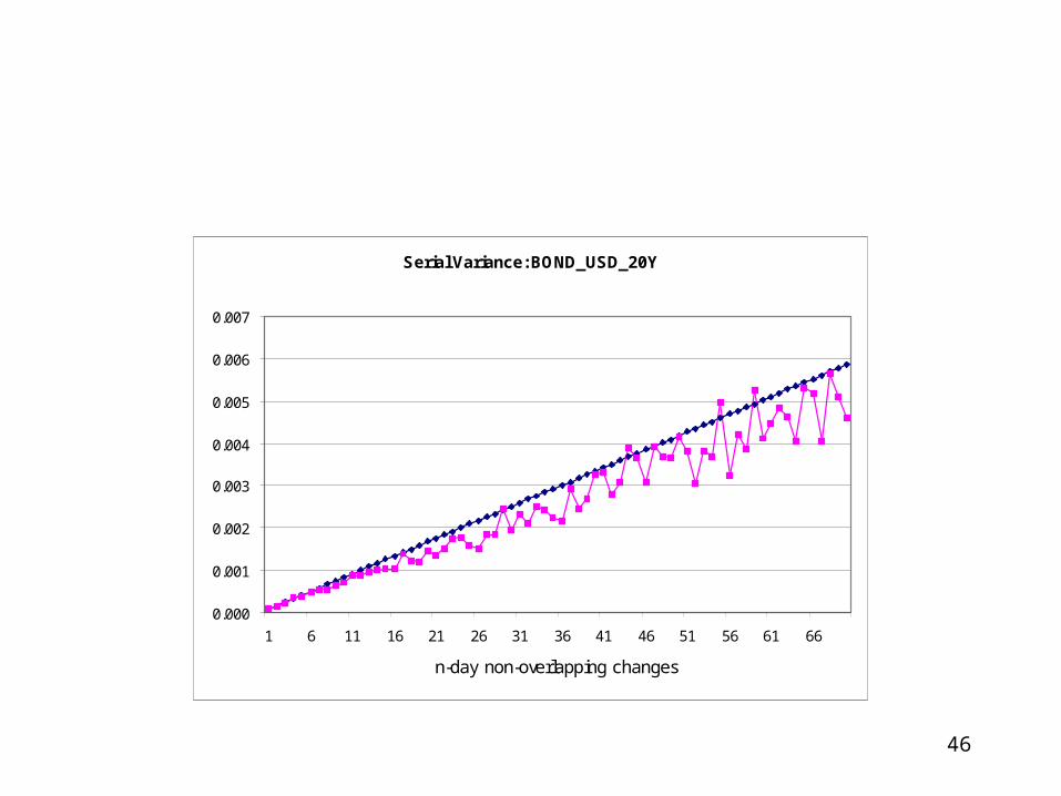
Serial Variance: BOND_USD_20Y
0.000
0.001
0.002
0.003
0.004
0.005
0.006
0.007
1 6 11 16 21 26 31 36 41 46 51 56 61 66
n-day non-overlapping changes

47
Serial Variance: BOND_USD_30Y
0.000
0.001
0.002
0.003
0.004
0.005
0.006
1 6 11 16 21 26 31 36 41 46 51 56 61 66
n-day non-overlapping changes

48
Empirical Observation
• The variance of short-maturity rates increases more than linearly with time
• The variance of long-maturity rates increases less than linearly with time
• The cross-over point is around the 2-year maturity

49
Two simultaneous mechanisms:
• The spring-constant mechanism (mean-reversion) makes the unconditional variance grow less than linearly.
• The presence of positive serial correlation would make the unconditional variance grow more than linearly.
• If this is correct this should be reflected in the serial auto-correlograms: positive serial correlation would make the variance of all rates grow super-linearly, but the strong springs at the long end would reduce this super-linear growth by introducing negative autocorrelation.
• Let’s check!
50
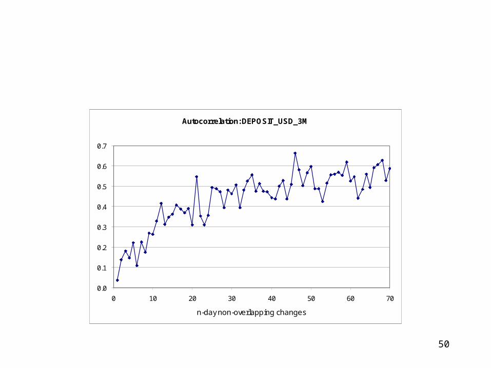
Autocorrelation: DEPOSIT_USD_3M
0.0
0.1
0.2
0.3
0.4
0.5
0.6
0.7
0 10 20 30 40 50 60 70
n-day non-overlapping changes

51
Autocorrelation: DEPOSIT_USD_6M
0.0
0.1
0.2
0.3
0.4
0.5
0.6
0.7
0 10 20 30 40 50 60 70
n-day non-overlapping changes

52
Autocorrelation: DEPOSIT_USD_1Y
0.0
0.1
0.2
0.3
0.4
0.5
0.6
0 10 20 30 40 50 60 70
n-day non-overlapping changes

53
Autocorrelation: BOND_USD_2Y
-0.1
0.0
0.1
0.2
0.3
0.4
0.5
0.6
0.7
0 10 20 30 40 50 60 70
n-day non-overlapping changes
54
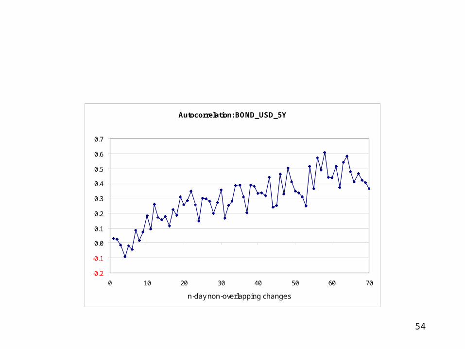
Autocorrelation: BOND_USD_5Y
-0.2
-0.1
0.0
0.1
0.2
0.3
0.4
0.5
0.6
0.7
0 10 20 30 40 50 60 70
n-day non-overlapping changes

55
Autocorrelation: BOND_USD_10Y
-0.2
-0.1
0.0
0.1
0.2
0.3
0.4
0 10 20 30 40 50 60 70
n-day non-overlapping changes

56
Autocorrelation: BOND_USD_20Y
-0.2
-0.1
0.0
0.1
0.2
0.3
0.4
0.5
0 10 20 30 40 50 60 70
n-day non-overlapping changes

57
Autocorrelation: BOND_USD_30Y
-0.2
-0.1
0.0
0.1
0.2
0.3
0.4
0 10 20 30 40 50 60 70
n-day non-overlapping changes

58
First conclusion:
• As anticipated, the serial autocorrelation becomes less and less positive (and eventually virtually disappears) as the maturity of the rate increases
• NB : there is no a priori contradiction with EMH! No comparison between forward and future rates.

59
Explanation for the strong positive auto-correlation
• Monetary authorities change short rates progressively and in the same direction for extended periods of time
• Conditional on the last move in the short rate being positive, the next move is more likely to be positive (and vice versa)
• The effect is stronger at the short end

60
Action plan:• Incorporate this information in such a way
that:– all the positive features recovered so far are
preserved (PCA)– the correct distribution of curvatures across
the yield curve is recovered– the variance and auto-correlation information
is incorporated in the new model– the model remains as non-parametric as
possible

61
The new algorithm:
• Sample a random day from U(1,N)
• Construct a ‘box’ of length n ahead of this day
• Add sequentially the increments associated with the days in the box, augmented by a drift term dependent on the curvature of the then-current yield curve (the spring constants)
• With intensity F jump out of the box and land on another random day.
• If after n draws the jump has not occurred, force the jump out of the box.
62
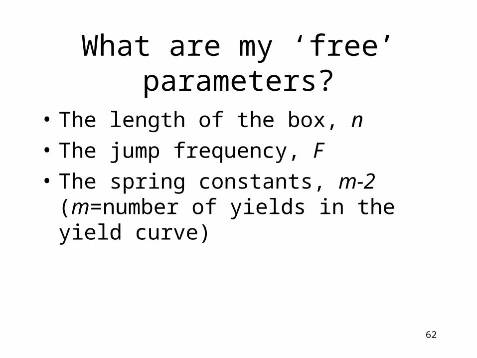
What are my ‘free’ parameters?
• The length of the box, n
• The jump frequency, F
• The spring constants, m-2 (m=number of yields in the yield curve)

63
How well does it work?
0.000
0.002
0.004
0.006
0.008
0.010
0.012
0.014
0 10 20 30 40 50 60
DEPOSIT_USD_3M
RealWorld
RealWorld

64
0.000
0.002
0.004
0.006
0.008
0.010
0.012
0.014
0 10 20 30 40 50 60
DEPOSIT_USD_6M
RealWorld
RealWorld

65
0.000
0.002
0.004
0.006
0.008
0.010
0.012
0.014
0 10 20 30 40 50 60
DEPOSIT_USD_1Y
RealWorld
RealWorld

66
0
0.002
0.004
0.006
0.008
0.01
0.012
0.014
0 10 20 30 40 50 60
BOND_USD_2Y
RealWorld
RealWorld

67
0.000
0.002
0.004
0.006
0.008
0.010
0.012
0.014
0.016
0 10 20 30 40 50 60
BOND_USD_5Y
RealWorld
RealWorld

68
0.000
0.001
0.002
0.003
0.004
0.005
0.006
0.007
0.008
0 10 20 30 40 50 60
BOND_USD_10Y
RealWorld
RealWorld

69
0.000
0.001
0.002
0.003
0.004
0.005
0.006
0 10 20 30 40 50 60
BOND_USD_20Y
RealWorld
RealWorld

70
0.000
0.001
0.001
0.002
0.002
0.003
0.003
0.004
0.004
0.005
0.005
0 10 20 30 40 50 60
BOND_USD_30Y
RealWorld
RealWorld

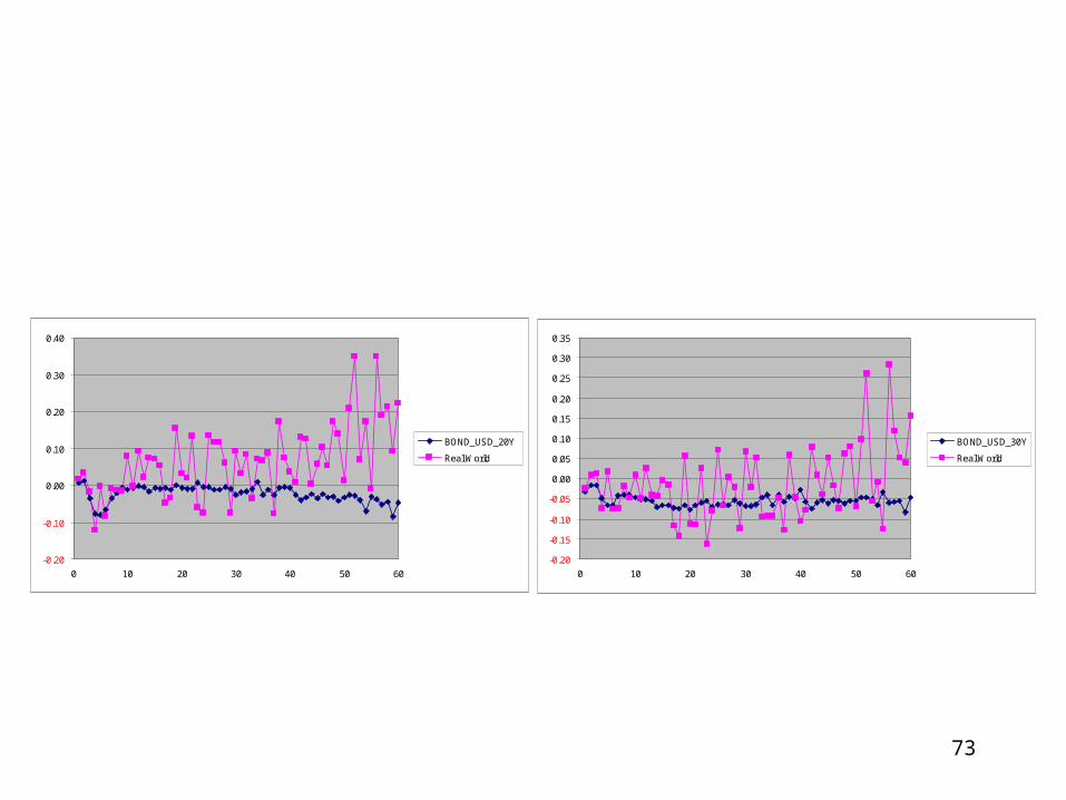
71
What about the auto-correlation?
• With the ‘usual’ (PCA-based) simulation methodologies it is 0 by construction
• With the ‘window’ methodology we propose it is clearly bounded by the length of the window
• So, if the window length is shorter than a ‘tightening cycle’, we expect the simulated serial auto-correlation to undershoot the experimental one
• Let’s see what happens…

72
0.00
0.10
0.20
0.30
0.40
0.50
0.60
0.70
0 10 20 30 40 50 60
DEPOSIT_USD_3M
Real World
-0.20
-0.10
0.00
0.10
0.20
0.30
0.40
0.50
0.60
0.70
0 10 20 30 40 50 60
DEPOSIT_USD_6M
Real World
-0.10
0.00
0.10
0.20
0.30
0.40
0.50
0.60
0 10 20 30 40 50 60
BOND_USD_2Y
Real World
-0.20
-0.10
0.00
0.10
0.20
0.30
0.40
0.50
0.60
0.70
0 10 20 30 40 50 60
BOND_USD_5Y
Real World
73
-0.20
-0.10
0.00
0.10
0.20
0.30
0.40
0 10 20 30 40 50 60
BOND_USD_20Y
Real World
-0.20
-0.15
-0.10
-0.05
0.00
0.05
0.10
0.15
0.20
0.25
0.30
0.35
0 10 20 30 40 50 60
BOND_USD_30Y
Real World

74
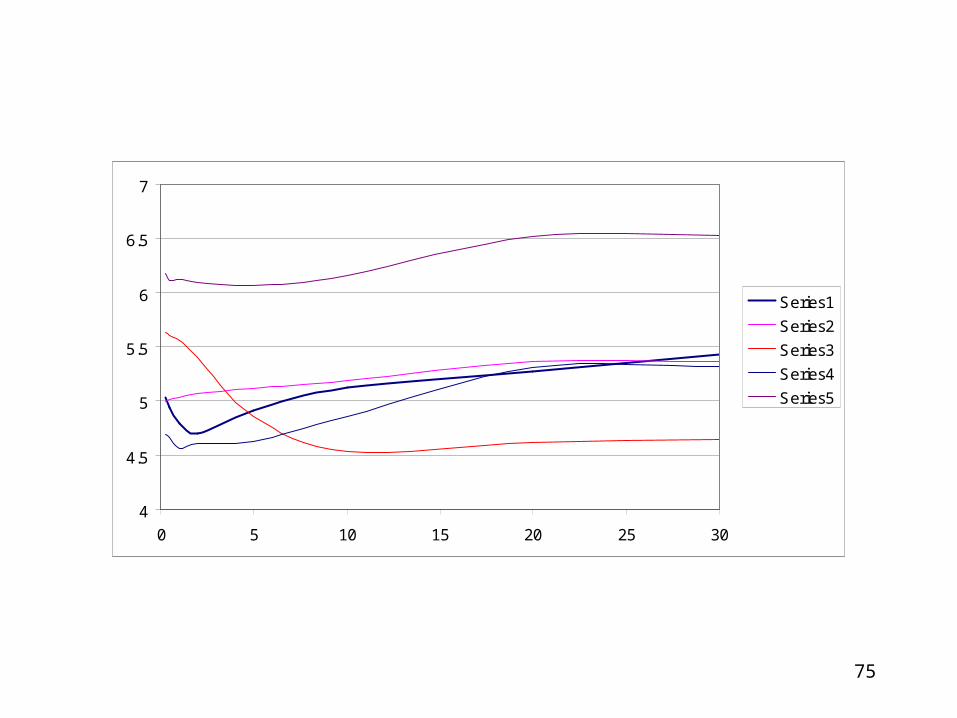
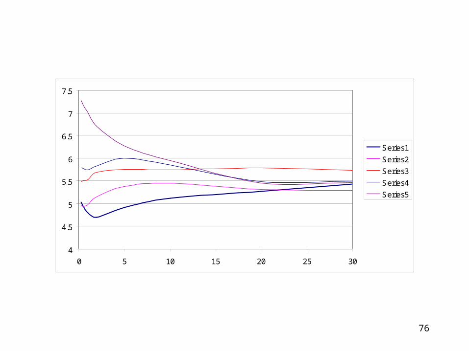
How well does it work?
4
4.5
5
5.5
6
6.5
0 5 10 15 20 25 30
Series1
Series2
Series3
Series4
Series5
75
4
4.5
5
5.5
6
6.5
7
0 5 10 15 20 25 30
Series1
Series2
Series3
Series4
Series5
76
4
4.5
5
5.5
6
6.5
7
7.5
0 5 10 15 20 25 30
Series1
Series2
Series3
Series4
Series5

77
4
4.2
4.4
4.6
4.8
5
5.2
5.4
5.6
5.8
6
0 5 10 15 20 25 30
Series1
Series2
Series3
Series4
Series5

78
Conclusions 1
• A simple procedure has been provided in order to generate future yield curves for real-measure simulations
• These can be used for – PFE calculations, – A&L management, – asset class comparison in investment portfolios,– assessment of hedging strategies...
79
Conclusions 2
The resulting yield curves have the properties that
• The PCA of the real data is recovered by construction
• The distribution of curvatures is similar to what observed in reality
• The unconditional variance of the yields and the serial auto-correlation are recovered well.
• A simple financial (trading) story can be associated to the proposed mechanism
• The resulting yield curves ‘look plausible’.