1 r as a tool in computational finance - nus risk management

1

R as a Tool in Computational Finance

John P. Nolan

Department of Mathematics and Statistics, American University, Washington, DC20016-8050 USA [email protected]

Key words: R Project, statistical analysis, programming, graphics

1.1 Introduction

R is a powerful, free program for statistical analysis and visualization. R hassuperb graphics capabilities and built-in functions to evaluate all commonprobability distributions, perform statistical analysis, and to do simulations.It also has a flexible programming language that allows one to quickly developcustom analyses and evaluate them. R includes standard numerical libraries:LAPACK for fast and accurate matrix multiplication, QUADPACK for nu-merical integration, and (univariate and multivariate) optimization routines.For compute intensive procedures, advanced users can call optimized codewritten in C or Fortran in a straightforward way, without having to writespecial interface code.

The R program is supported by a large international team of volunteerswho maintain versions of R for multiple platforms. In addition to the base Rprogram, there are hundreds of packages written for R. In particular, thereare dozens of packages for solving problems in finance. Information on im-plementations on obtaining the R program and documentation are given inAppendix 1.

A New York Times article by Vance (2009a) discussed the quick growthof R and reports that an increasing number of large companies are using Rfor analysis. Among those companies are Bank of America, Pfizer, Merck,InterContinental Hotels Group, Shell, Google, Novartis, Yale Cancer Center,Motorola, Hess. It is estimated in Vance (2009b) that over a quarter of amillion people now use R.

The following three simple examples show how to get free financial dataand how to begin to analyze it. Note that R uses the back arrow <- forassignment and that the > symbol is used as the prompt R uses for input.

2 John P. Nolan

price

Time

x

0 50 100 150 200 250

7090

110

return

Time

y

0 50 100 150 200 250

−0.05

0.05

Fig. 1.1. Closing price and return for IBM stock in 2008.

The following six lines of R code retrieve the adjusted closing price of IBMstock for 2008 from the web, compute the (logarithmic) return, plot both timeseries as shown in Figure 1.1, give a six number summary of the return data,and then finds the upper quantiles of the returns.

> x <- get.stock.price("IBM")

IBM has 253 values from 2008-01-02 to 2008-12-31

> y <- diff(log(x))

> ts.plot(x,main="price")

> ts.plot(y,main="return")

> summary(y)

Min. 1st Qu. Median Mean 3rd Qu. Max.

-0.060990 -0.012170 -0.000336 -0.000797 0.010620 0.091390

> quantile(y, c(.9,.95,.99) )

90% 95% 99%

0.02474494 0.03437781 0.05343545

The source code for the function get.stock.price and other functionsused below are given in Appendix 2. The next example shows more informa-tion for 3 months of Google stock prices, using the function get.stock.data

that retrieves stock information that includes closing/low/high prices as wellas volume.

> get.stock.data("GOOG",start.date=c(10,1,2008),stop.date=c(12,31,2008))

1 R as a Tool in Computational Finance 3

Google prices − Q4 2008

price

($)

0 10 20 30 40 50 60

300

350

400

highcloselow

Volume

Millio

n

050

150

Fig. 1.2. Google stock prices and volume in the 4th quarter of 2008.

GOOG has 64 values from 2008-10-01 to 2008-12-31

> par(mar=c(1,4,2,2)) # graphing option

> num.fig <- layout(matrix(c(1,2)),heights=c(5,2)) # setup a multiplot

> ts.plot(x$Close,ylab="price (in $)",main="Google prices - 4th quarter 2008")

> lines(x$Low,col="red")

> lines(x$High,col="blue")

> legend(45,400,c("high","close","low"),lty=1,col=c("blue","black","red"))

> barplot(x$Volume/100000,ylab="Million",col="lightblue",main="\nVolume")

Another function get.portfolio.returns will retrieve multiple stocksin a portfolio. Dates are aligned and a matrix of returns is the results. Thefollowing code retrieves the returns from IBM, General Electric, Ford andMicrosoft and produces scatter plots of the each pair of stocks. The last twocommands show the mean return and covariance of the returns

> x <- get.portfolio.returns( c("IBM","GE","Ford","MSFT") )


GE has 253 values from 2008-01-02 to 2008-12-31

Ford has 253 values from 2008-01-02 to 2008-12-31

MSFT has 253 values from 2008-01-02 to 2008-12-31

253 dates with values for all stocks, 252 returns calculated

> pairs(x)

> str(x)

’data.frame’: 252 obs. of 4 variables:

4 John P. Nolan

$ IBM : num 0.00205 -0.03665 -0.01068 -0.02495 0.00742 ...

$ GE : num 0.00118 -0.02085 0.00391 -0.02183 0.01128 ...

$ Ford: num -0.01702 -0.00862 -0.00434 -0.02643 0.00889 ...

$ MSFT: num 0.00407 -0.02823 0.00654 -0.03405 0.0293 ...

> mean(x)

IBM GE Ford MSFT

-0.0007974758 -0.0030421414 -0.0002416205 -0.0022856306

> var(x)

IBM GE Ford MSFT

IBM 0.0005138460 0.0005457266 0.0001258669 0.0004767922

GE 0.0005457266 0.0012353023 0.0003877436 0.0005865461

Ford 0.0001258669 0.0003877436 0.0016194549 0.0001845064

MSFT 0.0004767922 0.0005865461 0.0001845064 0.0009183715

The rest of this paper is organized as follows. Section 1.2 gives a briefintroduction to the R language, Section 1.3 gives several examples of using Rin finance, and Section 1.4 discusses the advantages and disadvantages of opensource vs. commercial software. Finally, the two appendices give informationon obtaining the R program and the R code used to obtain publicly availabledata on stocks.

1.2 Overview/tutorial of the R language

This section is a brief introduction to R. It is assumed that the reader hassome basic programming skills; this is not intended to teach programmingfrom scratch. You can find basic help within the R program by using thequestion mark before a command: ?plot (alternatively help("plot")) willgive a description of the plot command, with some examples at the bottomof the help page. Appendix 1 gives information on more documentation.

One powerful feature of R is that operations and functions are vectorized.This means one can perform calculations on a set of values without having toprogram loops. For example, 3*sin(x)+y will return a single number if x andy are single numbers, but a vector if x and y are vectors. (There are rules forwhat to do if x and y have different lengths, see below.)

A back arrow <-, made from a less than sign and a minus sign, is usedfor assignment. The equal sign is used for other purposes, e.g. specifying atitle in the plots above. Variable and function names are case sensitive, so X

and x refer to different variables. Such identifiers can also contain periods,e.g. get.stock.price. Comments can be included in your R code by using a# symbol; everything on the line after the # is ignored. Statements can beseparated by a semicolon within a line, or placed on separate lines without aseperator.


IBM

−0.10 0.00 0.10 −0.10 0.00 0.10

−0.

050.

000.

05

−0.

100.

000.

10

GE

Ford

−0.

10.

10.

3

−0.05 0.00 0.05

−0.

100.

000.

10

−0.1 0.1 0.3

MSFT

Fig. 1.3. Pairwise scatter plots of returns for 4 stocks.

1.2.1 Data types and arithmetic

Variables are defined at run time, not by a formal declaration. The type of avariable is determined by the type of the expression that defines it, and canchange from line to line. There are many data types in R. The one we willwork with most is the numeric type double (double precision floating pointnumbers). The simplest numeric type is a single value, e.g. x <- 3. Mostof the time we will be working with vectors, for example, x <- 1:10 givesthe sequence from 1 to 10. The statement x <- seq(-3,3,0.1) generatesan evenly spaced sequence from -3 to 3 in steps of size 0.1. If you have anarbitrary list of numbers, use the combine command, abbreviated c(...), e.g.x<- c(1.5, 8.7, 3.5, 2.1, -8) defines a vector with 5 elements.

6 John P. Nolan

You access the elements of a vector by using subscripts enclosed in squarebrackets: x[1],x[i], etc. If i is a vector, x[i] will return a vector of values.For example, x[3:5] will return the vector c(x[3],x[4],x[5]).

The normal arithmetic operations are defined: +,−, ∗, /. The power func-tion xp is x^ p. A very useful feature of R is that almost all operations andfunctions work on vectors elementwise: x+y will add the components of x andy, x*y will multiply the components of x and y, x^ 2 will square each ele-ment of x, etc. If two vectors are of different lengths in vector operations,the shorter one is repeated to match the length of the longer. This makesgood sense in some cases, e.g. x+3 will add 3 to each element of x, but canbe confusing in other cases, e.g. 1:10 + c(1,0) will result in the vector c(2,2,4,4,6,6,8,8,10,10).

Matrices can be defined with the matrix command: a <- matrix( c(1,5,

4,3,-2,5), nrow=2, ncol=3) defines a 2 × 3 matrix, filled with the valuesspecified in the first argument (by default, values are filled in one column ata time; this can be changed by using the byrow=TRUE option in the matrix

command). Here is a summary of basic matrix commands:

a + b adds entries element-wise (a[i,j]+b[i,j]),a * b is element by element (not matrix) multiplication (a[i,j]*b[i,j]),a %*% b is matrix multiplication,solve(a) inverts a,solve(a,b) solves the matrix equation a x = b,t(a) transposes the matrix a,dim(a) gives dimensions (size) of a,pairs(a) shows a matrix of scatter plots for all pairs of columns of a,a[i,] selects row i of matrix a,a[,j] selects column j of matrix a,a[1:3,1:5] selects the upper left 3× 5 submatrix of a.

Strings can be either a single value, e.g. a <- "This is one string", orvectors, e.g. a <- c("This", "is", "a", "vector", "of", "strings").

Another common data type in R is a data frame. This is like a matrix,but can have different types of data in each column. For example, read.tableand read.csv return data frames. Here is an example where a data frame isdefined manually, using the cbind command, which “column binds” vectorstogether to make a rectangular array.

name <- c("Peter","Erin","Skip","Julia")

age <- c(25,22,20,24)

weight <- c(180,120,160,130)

info <- data.frame(cbind(name,age,weight))

A more flexible data type is a list. A list can have multiple parts, and eachpart can be a different type and length. Here is a simple example:


x <- list(customer="Jane Smith",purchases=c(93.45,18.52,73.15),

other=matrix(1:12,3,4))

You access a field in a list by using $, e.g. x$customer or x$purchases[2],etc.

R is object oriented with the ability to define classes and methods, but wewill not go into these topics here. You can see all defined objects (variables,functions, etc.) by typing objects( ). If you type the name of an object, Rwill show you it’s value. If the data is long, e.g. a vector or a list, use thestructure command str to see a summary of what the object is.

R has standard control statements. A for loop lets you loop througha body of code a fixed number of times, while loops let you loop until acondition is true, if statements let you execute different statements dependingon some logical condition. Here are some basic examples. Brackets are usedto enclose blocks of statements, which can be multiline.

sum <- 0

for (i in 1:10) {sum <- sum + x[i] }

while (b > 0) { b <- b - 1 }

if (a < b) { print("b is bigger") }

else { print("a is bigger") }

1.2.2 General Functions

Functions generally apply some procedure to a set of input values and returna value (which may be any object). The standard math functions are built in:log, exp, sqrt, sin, cos, tan, etc. and we will not discuss them specif-ically. One very handy feature of R functions is the ability to have optionalarguments and to specify default values for those optional arguments. A sim-ple example of an optional argument is the log function. The default operationof the statement log(2) is to compute the natural logarithm of 2. However,by adding an optional second argument, you can compute a logarithm to anybase, e.g. log(2,base=10) will compute the base 10 logarithm of 2.

There are hundreds of functions in R, here are some common functions:

8 John P. Nolan

function name descriptionseq(a,b,c) defines a sequence from a to b in steps of size csum(x) sums the terms of a vectorlength(x) length of a vectormean(x) computes the meanvar(x) computes the variancesd(x) computes the standard deviation of xsummary(x) computes the 6 number summary of x (min, quartiles, mean, max)diff(x) computes successive differences xi − xi−1

c(x,y,z) combine into a vectorcbind(x,y,...) “bind” x, y,... into the columns of a matrixrbind(x,y,...) “bind” x, y,... into the rows of a matrixlist(a=1,b="red",...) define a list with components a, b, ...plot(x,y) plots the pairs of points in x and y (scatterplot)points(x,y) adds points to existing plotlines(x,y) adds lines/curves to existing plotts.plot(x) plots the values of x as a times seriestitle("abc") adds a title to an existing plotpar(...) sets parameters for graphing, e.g. par(mfrow=c(2,2)) creates a

2 by 2 matrix of plotslayout(...) define a multiplotscan(file) read a vector from an ascii fileread.table(file) read a table from an ascii fileread.csv(file) read a table from an Excel formated fileobjects() lists all objectsstr(x) shows the structure of an objectprint(x) prints the single object xcat(x,...) prints multiple objects, allows simple stream formattingsprintf(format,...) C style formatting of output

1.2.3 Probability distributions

The standard probability distributions are built into R. Here are the abbre-viations used for common distributions in R:

name distributionbinom binomialgeom geometricnbinom negative binomialhyper hypergeometricnorm normal/Gaussianchisq χ2

t Student tf Fcauchy Cauchy distribution


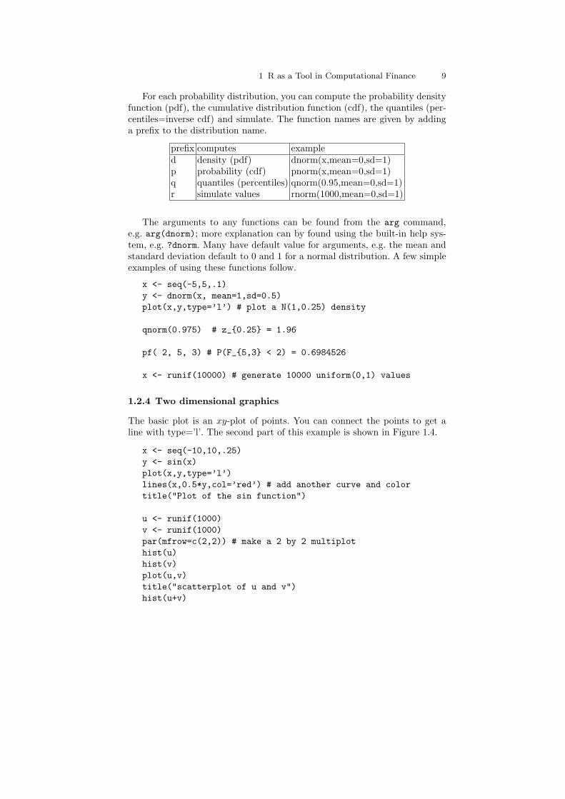
For each probability distribution, you can compute the probability densityfunction (pdf), the cumulative distribution function (cdf), the quantiles (per-centiles=inverse cdf) and simulate. The function names are given by addinga prefix to the distribution name.

prefix computes exampled density (pdf) dnorm(x,mean=0,sd=1)p probability (cdf) pnorm(x,mean=0,sd=1)q quantiles (percentiles) qnorm(0.95,mean=0,sd=1)r simulate values rnorm(1000,mean=0,sd=1)

The arguments to any functions can be found from the arg command,e.g. arg(dnorm); more explanation can by found using the built-in help sys-tem, e.g. ?dnorm. Many have default value for arguments, e.g. the mean andstandard deviation default to 0 and 1 for a normal distribution. A few simpleexamples of using these functions follow.

x <- seq(-5,5,.1)

y <- dnorm(x, mean=1,sd=0.5)

plot(x,y,type=’l’) # plot a N(1,0.25) density

qnorm(0.975) # z_{0.25} = 1.96

pf( 2, 5, 3) # P(F_{5,3} < 2) = 0.6984526

x <- runif(10000) # generate 10000 uniform(0,1) values

1.2.4 Two dimensional graphics

The basic plot is an xy-plot of points. You can connect the points to get aline with type=’l’. The second part of this example is shown in Figure 1.4.

x <- seq(-10,10,.25)

y <- sin(x)

plot(x,y,type=’l’)

lines(x,0.5*y,col=’red’) # add another curve and color

title("Plot of the sin function")

u <- runif(1000)

v <- runif(1000)

par(mfrow=c(2,2)) # make a 2 by 2 multiplot

hist(u)

hist(v)

plot(u,v)

title("scatterplot of u and v")

hist(u+v)

10 John P. Nolan

Histogram of u

u

Freq

uenc

y

0.0 0.2 0.4 0.6 0.8 1.0

020

4060

8010

0

Histogram of v

v

Freq

uenc

y

0.0 0.2 0.4 0.6 0.8 1.0

020

4060

8010

0

0.0 0.2 0.4 0.6 0.8 1.0

0.0

0.2

0.4

0.6

0.8

1.0

u

v

scatterplot of u and v Histogram of u + v

u + v

Freq

uenc

y

0.0 0.5 1.0 1.5 2.0

050

100

150

Fig. 1.4. Multiplot showing histograms of u, v, u+ v, and a scatter plot of (u, v).

There are dozens of options for graphs, including different plot symbols,legends, variable layout of multiple plots, annotations with mathematical sym-bols, trellis/lattice graphics, etc.

You can export graphs to a file in multiple formats using “File”, “Saveas”, and select type (jpg, postscript, png, etc.)

1.2.5 Three dimensional graphics

You can generate basic 3D graphs in standard R using the commands persp,contour and image. The first gives a “perspective” plot of a surface, thesecond gives a standard contour plot and the third gives a color coded contourmap. The examples below show simple cases; there are many more options.For static graphs, there are three functions: All three use a vector of x values,a vector of y values, and and matrix z of heights, e.g. z[i,j]<-f(x[i],y[j]).Here is one example where such a matrix is defined using the function f(x, y) =1/(1 + x2 + 3y2), and then the surface is plotted.

x <- seq(-3,3,.1) # a vector of length 61

y <- x

# allocate a 61 x 61 matrix and fill with f(x,y) values

z <- matrix(0,nrow=61,ncol=61)

for (i in 1:61) {

for (j in 1:61) {


xy

z

0.1

0.1

0.2

0.3

0.4 0.5

0.6

−3 −1 0 1 2 3

−3

−1

01

23

Fig. 1.5. A surface and contour plot.

z[i,j] <- 1/(1+x[i]^2 + 3*y[j]^2)

}

}

par(mfrow=c(2,2),pty=’s’) # set graphics parameters

persp(x,y,z,theta=30,phi=30) # plot the surface

contour(x,y,z)

image(x,y,z)

For clarity, we have used a standard double loop to fill in the z matrixabove, one could do it more compactly and quickly using the outer function.You can find more information about options by looking at the help page foreach command, e.g. ?persp will show help on the persp command. At thebottom of most help pages are some examples using that function. A wideselection of graphics can be found by typing demo(graphics).

There is a recent R package called rgl that can be used to draw dynamic3D graphs that can be interactively rotated and zoomed in/out using themouse. This package interfaces R to the OpenGL library; see the section onPackages below for how to install and load rgl. Once that is done, you canplot the same surface as above with

rgl.surface(x,y,z,col="blue")

This will pop up a new window with the surface. Rotate by using the leftmouse button: hold it down and move the surface, release to freeze in thatposition. Holding the right mouse button down allows you to zoom in andout. You can print or save an rgl graphic to a file using the rgl.snapshot

function (use ?rgl.snapshot for help).

12 John P. Nolan

1.2.6 Obtaining financial data

If you have data in a file in ascii form, you can read it with one of the R readcommands:

• scan("test1.dat") will read a vector of data from the specified file infree format.

• read.table("test2.dat") will read a matrix of data, assuming one rowper line.

• read.csv("test3.csv") will read a comma separate value file (Excel for-mat).

The examples in the first section and those below use R functions devel-oped for a math finance class taught at American University to retrieve stockdata from the Yahoo finance website. Appendix 2 lists the source code thatimplements the following three functions:

• get.stock.data: Get a table of information for the specified stock duringthe given time period. A data frame is returned, with Date, Open, High,Low, Close,Volume, and Adj.Close fields.

• get.stock.price: Get just the adjusted closing price for a stock.• get.portfolio.returns: Retrieve stock price data for each stock in a

portfolio (a vector of stock symbols). Data is merged into a data frameby date, with a date kept only if all the stocks in the portfolio have priceinformation on that date.

All three functions require the stock ticker symbol for the company,e.g.“IBM” for IBM, “GOOG” for Google, etc. Symbols can be looked uponline at www.finance.yahoo.com/lookup. Note that the function defaultsto data for 2008, but you can select a different time period by specifying startand stop date, e.g. get.stock.price("GOOG",c(6,1,2005),c(5,31,2008))will give closing prices for Google from June 1, 2005 to May 31, 2008.

If you have access to the commercial Bloomberg data service, there is anR package named RBloomberg that will allow you to access that data withinR.

1.2.7 Script windows and writing your own functions

If you are going to do some calculations more than once, it makes sense todefine a function in R. You can then call that function to perform that taskany time you want. You can define a function by just typing it in at thecommand prompt, and then call it. But for all but the simplest functions,you will find to more convenient to enter the commands into a file using aneditor. The default file extension is .R. To run those commands, you can eitheruse the source command, e.g. source("mycommands.R"), or use the top levelmenu: “File”, then “Source R code”, then select the file name from the pop-upwindow.


There is a built in editor within R that is convenient to use. To enter yourcommands, click on “File” in the top level menu, then “New script”. Typein your commands, using simple editing. To execute a block of commands,highlight them with the cursor, and then click on the “run line or selection”icon on the main menu (it looks like two parallel sheets of paper). You cansave scripts (click on the diskette icon or use CTRL-S), and open them (fromthe “File” menu or with the folder icon). If you want to change the commandsand functions in an existing script, use “File”, then “Open script”.

Here is a simple example that fits the (logarithmic) returns of price data inS with a normal distribution, and uses that to compute Value at Risk (VaR)from that fit.

compute.VaR <- function( S, alpha, V, T ){

# compute a VaR for the price data S at level alpha, value V

# and time horizon T (which may be a vector)

ret <- diff(log(S)) # return = log(S[i]/S[i-1])

mu <- mean(ret)

sigma <- sd(ret)

cat("mu=",mu," sigma=",sigma," V=",V,"\n")

for (n in T) {

VaR <- -V * ( exp(qnorm( alpha, mean=n*mu, sd=sqrt(n)*sigma)) - 1 )

cat("T=",n, " VaR=",VaR, "\n")}

}

Applying this to Google’s stock price for 2008, we see the mean and standarddeviation of the returns. With an investment of value V=$1000, and 95%confidence level, the projected VaRs for 30, 60, and 90 days are:

> price <- get.stock.price( "GOOG" )


> compute.VaR( price, 0.05, 1000, c(30,60,90) )

mu= -0.003177513 sigma= 0.03444149 V= 1000

T= 30 VaR= 333.4345

T= 60 VaR= 467.1254

T= 90 VaR= 561.0706

In words, there is a 5% chance that we will lose more than $333.43 on our$1000 investment in the next 30 days. Banks use these kinds of estimates tokeep reserves to cover loses.

1.3 Examples of R code for finance

The first section of this paper gave some basic examples on getting financialdata, computing returns, plotting and basic analysis. In this section we brieflyillustrate a few more examples of using R to analyze financial data.

14 John P. Nolan

1.3.1 Option pricing

For simplicity, we consider the Black-Scholes option pricing formula. The fol-lowing code computes the value V of a call option for an asset with currentprice S, strike price K, risk free interest rate r, time to maturity T and volatil-ity σ. It also computes the “Greek” delta: ∆ = dV/dS, returning the valueand delta in a named list.

call.optionBS <- function(S,K,r,T,sigma) {

d1 <- (log(S/K)+(r+sigma^2/2)*T )/ (sigma*sqrt(T))

d2 <- (log(S/K)+(r-sigma^2/2)*T )/ (sigma*sqrt(T))

return(list(value=S*pnorm(d1)-K*pnorm(d2),delta=pnorm(d1)))}

> call.optionBS( 100, 105, .02, 90, .1 )

$value

[1] 2.918652

$delta

[1] 0.9898371

> a <- call.optionBS( 100,105,.02, 0:90,.1)

> ts.plot(rev(a$value),main="Black-Scholes call option",

xlab="day",ylab="value")

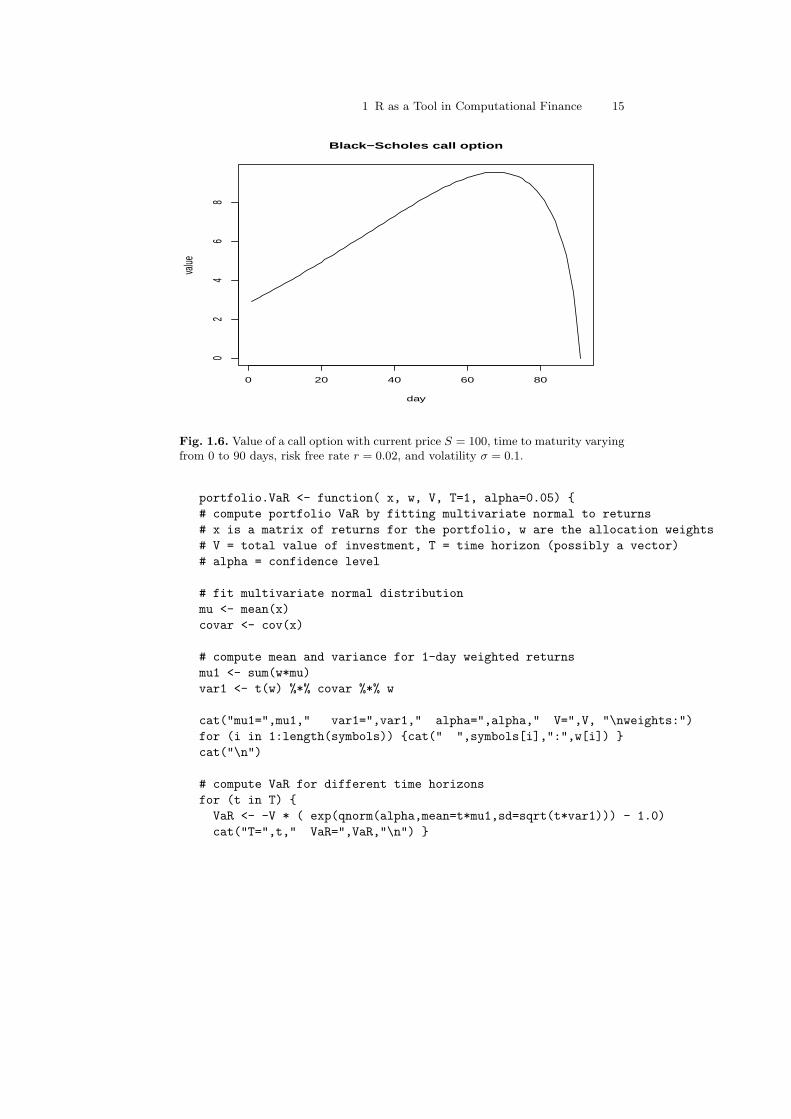
When the current price is S = 100, the strike price is K = 105, interest rater = 0.2, T = 90 days to maturity and volatility σ = 0.1, the Black-Scholesprice for a call option is 2.92. Also, the delta is 0.9898, meaning that if the priceS increases by $1, then the price of the option will increase by about $0.99.The delta values are used in hedging. The last three lines of the code abovecompute the price of a call option for varying days until maturity, startingat $2.92 for 90 days until maturity, increasing over time and reaching a maxat around day 68 where there is higher uncertainty about what the price willbe at day 90, then finally dropping to $0 at the last day. See Figure 1.6.Note that this last example works without changing the code because R usesvectorization.

1.3.2 Value-at-Risk for a portfolio

Above we looked at a function to compute Value-at-Risk (VaR) for a singleasset. We can generalize this to a static portfolio of N assets, with proportionwi of the wealth in asset i. Large financial institutions are required by theBasel II Accords (see Bank for International Settlements (2009)) to regularlycompute VaR and to hold capital reserves to cover losses determined by thesenumbers. (In practice, one may adjust the weights dynamically, to maximizereturn or minimize risk based on performance of the individual assets.) Asabove, we will assume that the (logarithmic) returns are multivariate normal.This makes the problem easy, but unrealistic (see below).


Black−Scholes call option

day

value

0 20 40 60 80

02

46

8

Fig. 1.6. Value of a call option with current price S = 100, time to maturity varyingfrom 0 to 90 days, risk free rate r = 0.02, and volatility σ = 0.1.

portfolio.VaR <- function( x, w, V, T=1, alpha=0.05) {

# compute portfolio VaR by fitting multivariate normal to returns

# x is a matrix of returns for the portfolio, w are the allocation weights

# V = total value of investment, T = time horizon (possibly a vector)

# alpha = confidence level

# fit multivariate normal distribution

mu <- mean(x)

covar <- cov(x)

# compute mean and variance for 1-day weighted returns

mu1 <- sum(w*mu)

var1 <- t(w) %*% covar %*% w

cat("mu1=",mu1," var1=",var1," alpha=",alpha," V=",V, "\nweights:")

for (i in 1:length(symbols)) {cat(" ",symbols[i],":",w[i]) }

cat("\n")

# compute VaR for different time horizons

for (t in T) {

VaR <- -V * ( exp(qnorm(alpha,mean=t*mu1,sd=sqrt(t*var1))) - 1.0)

cat("T=",t," VaR=",VaR,"\n") }

16 John P. Nolan

}

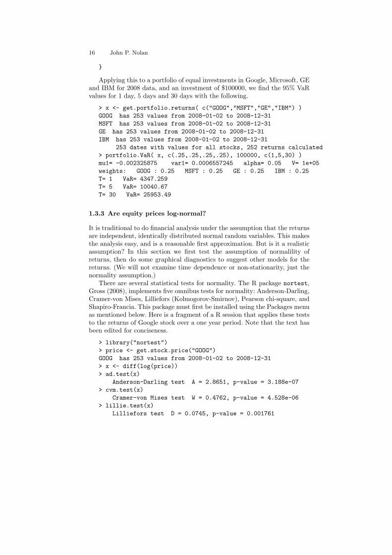
Applying this to a portfolio of equal investments in Google, Microsoft, GEand IBM for 2008 data, and an investment of $100000, we find the 95% VaRvalues for 1 day, 5 days and 30 days with the following.

> x <- get.portfolio.returns( c("GOOG","MSFT","GE","IBM") )


MSFT has 253 values from 2008-01-02 to 2008-12-31

GE has 253 values from 2008-01-02 to 2008-12-31


253 dates with values for all stocks, 252 returns calculated

> portfolio.VaR( x, c(.25,.25,.25,.25), 100000, c(1,5,30) )

mu1= -0.002325875 var1= 0.0006557245 alpha= 0.05 V= 1e+05

weights: GOOG : 0.25 MSFT : 0.25 GE : 0.25 IBM : 0.25

T= 1 VaR= 4347.259

T= 5 VaR= 10040.67

T= 30 VaR= 25953.49

1.3.3 Are equity prices log-normal?

It is traditional to do financial analysis under the assumption that the returnsare independent, identically distributed normal random variables. This makesthe analysis easy, and is a reasonable first approximation. But is it a realisticassumption? In this section we first test the assumption of normalility ofreturns, then do some graphical diagnostics to suggest other models for thereturns. (We will not examine time dependence or non-stationarity, just thenormality assumption.)

There are several statistical tests for normality. The R package nortest,Gross (2008), implements five omnibus tests for normality: Anderson-Darling,Cramer-von Mises, Lilliefors (Kolmogorov-Smirnov), Pearson chi-square, andShapiro-Francia. This package must first be installed using the Packages menuas mentioned below. Here is a fragment of a R session that applies these teststo the returns of Google stock over a one year period. Note that the text hasbeen edited for conciseness.

> library("nortest")

> price <- get.stock.price("GOOG")


> x <- diff(log(price))

> ad.test(x)

Anderson-Darling test A = 2.8651, p-value = 3.188e-07

> cvm.test(x)

Cramer-von Mises test W = 0.4762, p-value = 4.528e-06

> lillie.test(x)

Lilliefors test D = 0.0745, p-value = 0.001761


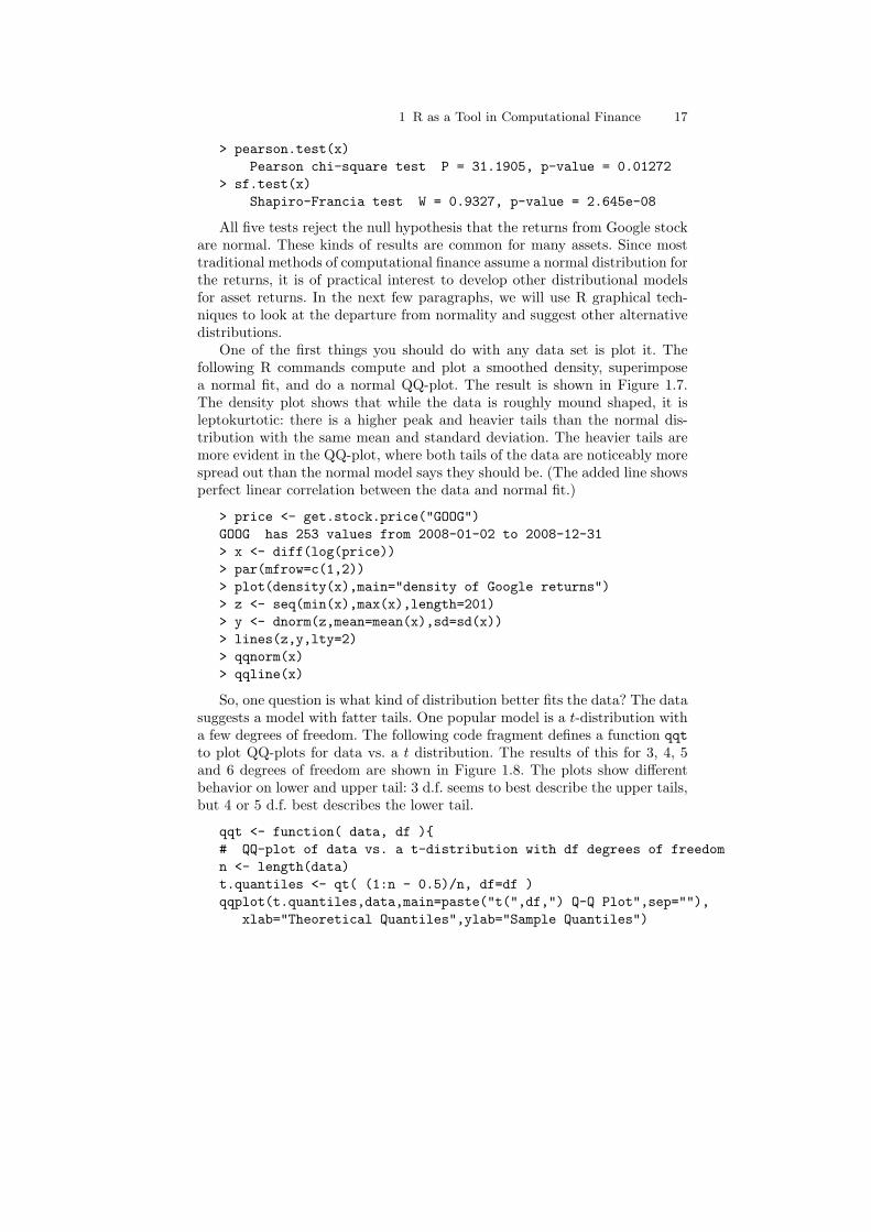
> pearson.test(x)

Pearson chi-square test P = 31.1905, p-value = 0.01272

> sf.test(x)

Shapiro-Francia test W = 0.9327, p-value = 2.645e-08

All five tests reject the null hypothesis that the returns from Google stockare normal. These kinds of results are common for many assets. Since mosttraditional methods of computational finance assume a normal distribution forthe returns, it is of practical interest to develop other distributional modelsfor asset returns. In the next few paragraphs, we will use R graphical tech-niques to look at the departure from normality and suggest other alternativedistributions.

One of the first things you should do with any data set is plot it. Thefollowing R commands compute and plot a smoothed density, superimposea normal fit, and do a normal QQ-plot. The result is shown in Figure 1.7.The density plot shows that while the data is roughly mound shaped, it isleptokurtotic: there is a higher peak and heavier tails than the normal dis-tribution with the same mean and standard deviation. The heavier tails aremore evident in the QQ-plot, where both tails of the data are noticeably morespread out than the normal model says they should be. (The added line showsperfect linear correlation between the data and normal fit.)

> price <- get.stock.price("GOOG")


> x <- diff(log(price))

> par(mfrow=c(1,2))

> plot(density(x),main="density of Google returns")

> z <- seq(min(x),max(x),length=201)

> y <- dnorm(z,mean=mean(x),sd=sd(x))

> lines(z,y,lty=2)

> qqnorm(x)

> qqline(x)

So, one question is what kind of distribution better fits the data? The datasuggests a model with fatter tails. One popular model is a t-distribution witha few degrees of freedom. The following code fragment defines a function qqt

to plot QQ-plots for data vs. a t distribution. The results of this for 3, 4, 5and 6 degrees of freedom are shown in Figure 1.8. The plots show differentbehavior on lower and upper tail: 3 d.f. seems to best describe the upper tails,but 4 or 5 d.f. best describes the lower tail.

qqt <- function( data, df ){

# QQ-plot of data vs. a t-distribution with df degrees of freedom

n <- length(data)

t.quantiles <- qt( (1:n - 0.5)/n, df=df )

qqplot(t.quantiles,data,main=paste("t(",df,") Q-Q Plot",sep=""),

xlab="Theoretical Quantiles",ylab="Sample Quantiles")

18 John P. Nolan

−0.15 0.00 0.10 0.20

05

1015

density of Google returns

N = 252 Bandwidth = 0.007315

Dens

ity

−3 −1 0 1 2 3

−0.10

−0.05

0.00

0.05

0.10

0.15

Normal Q−Q Plot

Theoretical Quantiles

Samp

le Qu

antile

s

Fig. 1.7. Google returns in 2008. The left plot shows smoothed density with dashedline showing the normal fit, and the right plot shows a normal QQ-plot.

qqline(data) }

# diagnostic plots for data with t distribution with 3,4,5,6 d.f.

par(mfrow=c(2,2))

for (df in 3:6) {

qqt(x,df)

}

There are many other models proposed for fitting returns, most of themhave heavier tails than the normal and some allow skewness. One reference forthese models is Rachev (2003). If the tails are really heavy, then the familyof stable distributions has many attractive features, including closure underconvolution (sums of stable laws are stable) and the Generalized Central LimitTheorem (normalized sums converge to a stable law).

A particularly difficult problem is how to model multivariate dependence.Once you step outside the normal model, it generally takes more than a co-variance matrix to describe dependence. In practice, a large portfolio withmany assets of different type can have very different behavior for different as-sets. Some returns may be normal, some t with different degrees of freedom,some a stable law, etc. Copulas are one method of dealing with multivariatedistributions, though the limited classes of copulas used in practice seems tohave misled people into thinking they had correctly modeled dependence. Inaddition to modeling complete joint dependence, there is research on modeling


−5 0 5

−0.

100.

000.

10

t(3) Q−Q Plot


Sam

ple

Qua

ntile

s

−6 −4 −2 0 2 4 6

−0.

100.

000.

10

t(4) Q−Q Plot


Sam

ple

Qua

ntile

s

−4 −2 0 2 4

−0.

100.

000.

10

t(5) Q−Q Plot


Sam

ple

Qua

ntile

s

−4 −2 0 2 4−

0.10

0.00

0.10

t(6) Q−Q Plot


Sam

ple

Qua

ntile

s

Fig. 1.8. QQ-plots of Google returns in 2008 for t distributions with 3, 4, 5 and 6degrees of freedom.

tail dependence. This is a less ambitious goal, but could be especially useful inmodeling extreme movements by multiple assets - an event that could causea catastrophic result.

Realistically modeling large portfolios is an important open problem. Therecent recession may have been prevented if practitioners and regulators hadbetter models for returns, and ways to effectively model dependence.

1.3.4 R packages for finance

Packages are groups of functions that are used to solve a particular problem.They can be written entirely in the R programming language, or coded inC or Fortran for speed and connected to R. There are many packages beingdeveloped to do different tasks. The rgl package to do interactive 3-D graphsand the nortest package to test normality were mentioned above. You candownload these for free and install them (only done once). You can then loadthem into the program (this must be done each time you start R).

There is an online list of packages useful for empirical finance, see Eddel-buettel (2009). This page has over 100 listings for R packages that are used

20 John P. Nolan

in computational finance, grouped by topics: regression models, time series,finance, risk management, etc.

Diethelm Wurtz and his group at the Econophysics Group at the Instituteof Theoretical Physics of ETH Zurich, have developed a free, large collectionof packages called Rmetrics. They have a simple way to install the wholeRmetrics package in two lines:

> source("http://www.rmetrics.org/Rmetrics.R")

> install.Rmetrics()

1.4 Open source R vs. commercial packages

We end with a brief comparison of the advantages and disadvantages of opensource R vs. commercial packages (matlab, Mathematica, SAS, etc.) Whilewe focus on R, the comments are generally applicable to other open sourceprograms.

Cost Open software is free, with no cost for obtaining the software or runningit on any number of machines. Anyone with a computer can use R -whether you work for a large company with a cumbersome purchasingprocess, are an amateur investor, or are a student in a major researchuniversity or in an inner city school, whether you live in Albania or inZambia. Commercial packages generally cost in the one to two thousanddollar range, making them beyond the reach of many.

Ease of installing and upgrading The R Project has done an excellentjob of making it easy to install the core system. It is also easy to quicklydownload and install packages. When a new version comes out, users caneither immediately install the new version, or continue to run an existingversion without fear of a license expiring. Upgrades are simple and free.

Verifiability Another advantage of open software is the ability to examinethe source code. While most users will not dig through the source code ofindividual routines, anyone can and someone eventually will. This meansthat algorithms can be verified by anyone with the interest. Code can befixed or extended by those who want to add capabilities. (If you’ve ever hita brick wall with a commercial package that does not work correctly, youwill appreciate this feature. Years ago, the author was using a multivariateminimization routine with box constraints from a well known commercialpackage. After many hours debugging, it was discovered that the problemwas in the minimization routine: it would sometimes search outside thespecified bounds, where the objective function was undefined. After daysof trying to get through to the people who supported this code, and pre-senting evidence of the problem, they eventually confirmed that it was anissue, but were unwilling to fix the problem or give any work-around.)

Documentation and support No one is paid to develop user friendly doc-umentation for R, so built-in documentation tends to be terse, making


sense to the cognesceti, but opaque to the novice. There is now a largeamount of documentation online and books on R, though the problemmay still be finding the specific information you want. There are multipleactive mailing lists, but with a very heterogeneous group of participants.There are novices struggling with basic features and R developers dis-cussing details of the internals of R. If a bug is found, it will get fixed,though the statement that “The next version of R will fix this problem”may not help much in the short run. Of course, commercial software sup-port is generally less responsive.

Growth There is a vibrant community of contributors to R. With literallythousands of people developing packages, R is a dynamic, growing pro-gram. If you don’t like the way a package works, you can write your own,either from scratch or by adapting an existing package from the availablesource code. A drawback of this distributed development model is thatR packages are of unequal quality. You may have to try various packagesand select those that provide useful tools.

Stability Software evolves over time, whether open source or commercial. Ina robust open source project like R, the evolution can be brisk, with newversions appearing every few months. While most of R is stable, there areoccasionally small changes that have unexpected consequences. Packagesthat used to work, can stop working when a new version comes out. Thiscan be a problem with commercial programs also: a few years ago matlabchanged the way mex programs were built and named. Toolboxes thatusers developed or purchased, sometimes at a significant cost, would nolonger work.

Certification Some applications, e.g. medical use and perhaps financial com-pliance work, may require that the software be certified to work correctlyand reproducibly. The distributed development and rapid growth of R hasmade it hard to do this. There is an effort among the biomedical users ofR to find a solution to this issue.

Institutional resistance In some institutions, IT staff may resist puttingfreeware on a network, for fear that it may be harmful. Also, they arewary of being held responsible for installing, maintaining, and updatingsoftware that is not owned/licensed by a standard company.

In the long run, it seems likely that R and other open source packages willsurvive and prosper. Because of their higher growth rate, they will eventuallyprovide almost all of the features of commercial products. When that pointwill be reached is unknown. In the classroom, where the focus is on learningand adaptability, the free R program is rapidly displacing other alternatives.

There is a new development in computing that is a blend of free, opensource software and commercial support. REvolution Computing (2008) offersversions of R that are optimized and validated, and have developed customextensions, e.g. parallel processing. This allows a user to purchase a purport-edly more stable, supported version of R. It will be interesting to watch where

22 John P. Nolan

this path leads; it may be a way to address the institutional resistance men-tioned above. Another company, Mango Solutions (2009) provides trainingin R, with specific courses R for Financial Data Analysis. A third company,Inference for R (2009), has an integrated development environment that doessyntax highlighting, R debugging, allows one to run R code from MicrosoftOffice applications (Excel, Word and PowerPoint), and other features. Finally,we mention the SAGE Project. SAGE (2008) is an open source mathematicssystem that includes R. In addition to the features of R, it includes sym-bolic capabilities to handle algebra, calculus, number theory, cryptography,and much more. Basically, it is a Python program that interfaces with over60 packages: R, Maxima, the Gnu Scientific Library, etc.

1.5 Appendix 1: Obtaining and installing R: R Projectand Comprehensive R Archive Network (CRAN)

The R Project’s website is www.r-project.org, where you can obtain theR program, packages, and even the source code for R. The ComprehensiveR Archive Network (CRAN) is a coordinated group of over 60 organizationsthat maintain servers around the world with copies of the R program (sim-ilar to the CTAN system for TEX). To download the R program, go to theR Project website and on the left side of the page, click on “CRAN”, selecta server near you, and download the version of R for your computer type.(Be warned: this is a large file, over 30 mb.) On Windows, the program nameis something like R-2.10.0-win32.exe, which is version 2.10.0 of R for 32-bitWindows; newer versions occur every few months and will have higher num-bers. After the file is on your computer, execute the program. This will gothrough the standard installation procedure. For a Mac, the download is auniversal binary file (.dmg) for either a PowerPC or an Intel based proces-sor. For linux, there are versions for debian, redhat, suse or ubuntu. The RProject provides free manuals that explain different parts of R. Start on theR homepage www.r-project.org and click on Manuals on the left side of thepage. A standard starting point is An Introduction to R, which is a PDF fileof about 100 pages. There are dozens of other manuals, some of which aretranslated to 13 different languages.

To download a package, it is easiest to use the GUI menu system within R.Select “Packages” from the main top menu, then select “Install package(s)”.You will be prompted to select a CRAN server from the first pop-up menu(pick one near you for speed), then select the package you want to installfrom the second pop-up menu. The system will go to the server, download acompressed form of the package, and install it on your computer. This partonly needs to be done once. Anytime you want to use that package, you haveto load it into your session. This is easy to do from the Packages menu: “Loadpackage...”, and then select the name of an installed package. You can also


use the library( ) command, as in the example with the nortest packageabove.

If you want to see the source code for R, once you are on the CRAN pages,click on the section for source code.

1.6 Appendix 2: R functions for retrieving finance data

Disclaimer: these functions are not guaranteed for accuracy, nor can we guar-antee the accuracy of the Yahoo data. They are very useful in a classroomsetting, but should not be relied on as a basis for investing.

# R programs for Math Finance class

# John Nolan, American University [email protected]

#######################################################################

get.stock.data <- function( symbol, start.date=c(1,1,2008),

stop.date=c(12,31,2008), print.info=TRUE ) {

# get stock data from yahoo.com for specified symbol in the

# specified time period. The result is a data.frame with columns for:

# Date, Open, High, Low, Close,Volume, Adj.Close

url <- paste("http://ichart.finance.yahoo.com/table.csv?a=",

start.date[1]-1,"&b=",start.date[2],"&c=",start.date[3],

"&d=",stop.date[1]-1,"&e=",stop.date[2],"&f=",stop.date[3],"&s=",

symbol,sep="")

x <- read.csv(url)

# data has most recent days first, going back to start date

n <- length(x$Date); date <- as.character(x$Date[c(1,n)])

if (print.info) cat(symbol,"has", n,"values from",date[2],"to",date[1],"\n")

# data is in reverse order from the read.csv command

x$Date <- rev(x$Date)

x$Open <- rev(x$Open)

x$High <- rev(x$High)

x$Low <- rev(x$Low)

x$Close <- rev(x$Close)

x$Volume <- rev(x$Volume)

x$Adj.Close <- rev(x$Adj.Close)

return(x) }

#######################################################################

get.stock.price <- function( symbol, start.date=c(1,1,2008),

stop.date=c(12,31,2008), print.info=TRUE ) {

# gets adjusted closing price data from yahoo.com for specified symbol

24 John P. Nolan

x <- get.stock.data(symbol,start.date,stop.date,print.info)

return(x$Adj.Close) }

#######################################################################

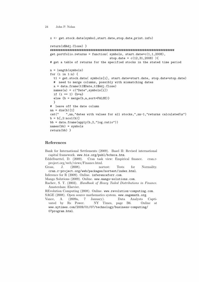
get.portfolio.returns = function( symbols, start.date=c(1,1,2008),

stop.date = c(12,31,2008) ){

# get a table of returns for the specified stocks in the stated time period

n = length(symbols)

for (i in 1:n) {

t1 = get.stock.data( symbols[i], start.date=start.date, stop.date=stop.date)

# need to merge columns, possibly with mismatching dates

a = data.frame(t1$Date,t1$Adj.Close)

names(a) = c("Date",symbols[i])

if (i == 1) {b=a}

else {b = merge(b,a,sort=FALSE)}

}

# leave off the date column

nn = dim(b)[1]

cat(" ",nn,"dates with values for all stocks,",nn-1,"returns calculated\n")

b = b[,2:ncol(b)]

bb = data.frame(apply(b,2,"log.ratio"))

names(bb) = symbols

return(bb) }

References

Bank for International Settlements (2009). Basel II: Revised internationalcapital framework. www.bis.org/publ/bcbsca.htm.

Eddelbuettel, D. (2009). Cran task view: Empirical finance. cran.r-project.org/web/views/Finance.html.

Gross, J. (2008). nortest: Tests for Normality.cran.r-project.org/web/packages/nortest/index.html.

Inference for R (2009). Online. inferenceforr.com.Mango Solutions (2009). Online. www.mango-solutions.com.Rachev, S. T. (2003). Handbook of Heavy Tailed Distributions in Finance.

Amsterdam: Elsevier.REvolution Computing (2008). Online. www.revolution-computing.com.SAGE (2008). Open source mathematics system. www.sagemath.org.Vance, A. (2009a, 7 January). Data Analysts Capti-

vated by Rs Power. NY Times, page B6. Online atwww.nytimes.com/2009/01/07/technology/business-computing/

07program.html.


Vance, A. (2009b, 8 January). R You Ready for R? NY Times website. Onlineat bits.blogs.nytimes.com/2009/01/08/r-you-ready-for-r/.

1 r as a tool in computational finance - nus risk management

Documents