1 query processing in the presence of limited source capabilities chen li information and computer...

1

Query Processing in the Presence

of Limited Source Capabilities

Chen LiInformation and Computer

ScienceUC Irvine

2

Information integration

Legacy database Plain text files

Biblio sever

Support seamless access to autonomous and heterogeneous information sources.

3

Mediation architecture

Mediator

Wrapper

Source 1

Wrapper Wrapper

Source 2 Source n

4

Limited Source Capabilities

Ullman DBSI

Knuth TeX

… …

author title

Get all books.

support “select * from R” queries

Traditional DBs

5

Limited source capabilities (cont)

Ullman DBSI

Knuth TeX

… …

author titleGiven an author,

return the books.

However, in many environments, complete scans of relations may not be possible

Reasons:

– Legacy databases or structured files: limited interfaces

– Security/Privacy

– Performance concerns

6

Example: Web search forms

www.imdb.com

7

Research summarySome of my work on query processing in the presence of limited source capabilities:

Generating a feasible plan for a query: demo SIGMOD'1998. Optimizing large-join queries: ICDT’1999. Describing source capabilities and computing capabilities of

mediators: SIGMOD'1999. Computing maximal answers to a query by borrowing

information from sources not in the query : ICDE'2000, TODS 2001.

Deciding whether all the answers to a query can be computed and testing relative query containment: ICDT'2001, Journal of VLDB.

Other work: e.g., answering queries using views with binding patterns [RSU95], query rewriting for semi-structured data [PV99], etc.

8

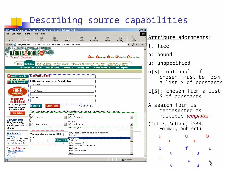
Attribute adornments:

f: free

b: bound

u: unspecified

o[S]: optional, if chosen, must be from a list S of constants

c[S]: chosen from a list S of constants

A search form is represented as multiple templates:

(Title, Author, ISBN, Format, Subject)

u u b u u

b f u u u

f b u u u

o[] u u o[] o[]

[SIGMOD’99]

Describing source capabilities

9

Binding patterns

Common source limitations Attributes with adornments:

— b: bound— f: free

Example: R(Author, Title)— Given an author, return the books.— R(Authorb, Titlef)

A relation can have multiple binding patterns.

10

Part I: Optimizing large-join queries Part II: Deciding whether all the

answers to a query can be computed

Rest of the talk

11

Given a query Q on relations with restrictions:

Can we answer Q?— I.e., find an executable plan to answer the

query while observing the source access patterns

How to answer Q efficiently?

Part I: Optimizing large-join queries

12

Example: three movie sources

R(Star, Movie)

Reeves The Matrix

Connery The Rock

… …

The Matrix Warner BrosAmerican Beauty

… …DreamWorks

S(Movie,Studio)

The Rock 1996

The Matrix

… …1999

T(Movie,Year)

13

“Find the movies made by Warner Bros. in 1999 and in which Keanu Reeves starred?”

SQL: SELECT MovieFROM R JOIN S JOIN TWHERE Star = ’reeves’ AND Studio = ’warner’ AND Year = 1999;

R(Star, Movie)

S(Movie,Studio)

T(Movie,Year)

reeves

1999

warner

Query Q

14

Answer Q

Plan P0

Star=reeves

R(Star, Movie)

Studio=warner

S(Movie,Studio)

Year=1999

T(Movie,Year)

Movie

15

What if limited source capabilities?

R(Starb, Movief): requires a Star name S(Movieb,Studiof): requires a Movie title T(Movieb,Yearf): requires a Movie title

16

Does P0 work?No! Since S and T do not support the queries.

Star=reeves Studio=warner Year=1999

R(Starb, Movief) S(Movieb,Studiof) T(Movieb,Yearf)

17

A feasible plan P1

Star=reeves


Reeves movies Reeves movies

by warner of 1999

Reeves moviesby warner

18

Another feasible plan P2

Star=reeves


Reeves movies

Reeves movies of 1999

Reeves movies of 1999 by warner

19

Question 1: query answerability

Given Q on relations with restrictions, can we process its conditions by accessing relations with legal patterns?

20

Consider SPJ Queries Select-project-join queries (conjunctive queries):

q(X) :- g1(X1),…, gn(Xn)— subgoal gi(Xi): gi is a relation, Xi is a tuple of

variables/constants Example:

SELECT MovieFROM R JOIN S JOIN TWHERE Star = ’reeves’ AND Studio = ’warner’

AND Year = 1999;q(M) :- R(reeves,M),S(M,warner),T(M,1999)

21

Algorithm “Inflationary”:Testing answerability of Q

R(Starb, Movief), S(Movieb,Studiof), T(Movieb,Yearf)

Check what subgoals can be processed given B

More subgoals can be processed

All subgoals are answerable, so Q is answerable

q(M) :- R(reeves,M),S(M,warner),T(M,1999)

More positions become bound: add {M} to B

M M M

Bound positions: B = {reeves, warner, 1999}

reeves warner 1999

22

Question 2: generate efficient plans?

Number of source accesses: 1 + 12 + 4 = 17

Plan P1


Consider number of source accesses.

1

Star=reeves

12

reeves movies reeves movies

by warner of 1999

4

reeves moviesby warner

23

Cost of plan P2Plan P2

1

star=reeves


12

reeves movies

1

reeves movies of 1999

reeves moviesby warner of 1999

Number of source accesses: 1 + 12 + 1 = 14

24

How to generate efficient plans?

Challenges:— Often source statistics hard to get— Search space different from a traditional optimizer (e.g.,

System-R) Ordering subgoals Considering left-deep trees versus bushy trees Deciding join methods (e.g., hash join, nested-loop join) Need to consider feasible plans!

Cost model: total number of source accesses— Reason: each source access is expensive!

network traffic/delay, dynamic source availability, source charges — Results extendable to more general cost models, e.g.:

25

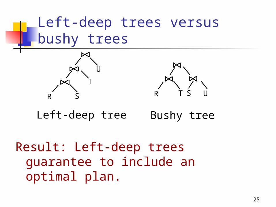
Left-deep trees versus bushy trees

SR

T

U

TR S U

Result: Left-deep trees guarantee to include an optimal plan.

Left-deep tree Bushy tree

26

Complexity The problem of finding the optimal feasible

plans is NP-hard— Proof: by reduction from the Vertex Cover

Problem Since the number of subgoals could be large,

we want approximation algorithms for finding near-optimal plans quickly

27

Case 1: no source statistics Algorithm CHAIN:

— Greedy approach— At each step, find a subgoal with the lowest cost

28

CHAIN

R(Studiob, Movief , Starf)S(Movieb,Yearf)

T(Starb,Addrf)Movie Star

2 movies 3 stars

Choose S next!

Collect source information as we process subgoals.

Murphy

Diaz

Reeves

Shrek

Shrek

Matrix

29

CHAIN: Properties

Does not need source statistics Polynomial time: O(n2), n is the number of

subgoals— Only needs results returned from the sources

It is n-competitive:Cost(PLANchain) <= n * Cost(PLANopt)

30

Case 2: source statistics available

Algorithm: PARTITION— Grouping approach: group subgoals into

clusters— Find an optimal subplan within each

cluster— Combine subplans to construct a plan

31

PARTITION

answerable subgoals given initial constants in Q

new answerable subgoals

new bound args

group 1

group 2

new answerable subgoals

new bound args

group k

…

optimal subplan p1

optimal subplan p2

optimal subplan pk

completeplan

32

PARTITION: Properties Need source statistics Guarantees an optimal plan if 1 or 2 clusters No bound when missing optimal plans

33

Performance analysis Test bed:

— 15 source relations; number of subgoals: 1 – 10— For each number of subgoals, ran 1000 random

queries— Other factors considered:

number of binding patterns for a relation number of constants in a query cardinalities of attributes

Results:— Both algorithms generate good plans— PARTITION takes more time than CHAIN— PARTITION generates better plans than CHAIN

34

Average probability of missing optimal plans:

• CHAIN <= 25%

• PARTITION <= 5%

Probability of missing optimal plans

Precentage of nonoptimal plans

0

5

10

15

20

25

30

35

40

45

1 2 3 4 5 6 7 8 9 10Number of subgoals

Pe

rce

nta

ge

(%

)

CHAIN

PARTITION

35

Average difference:

• CHAIN < 5%

• PARTITION < 2%

Difference from the optimal plans

Avg Difference from Optimal Plans

0

12

34

56

78

9

1 2 3 4 5 6 7 8 9 10

Number of subgoals

Dif

fere

nce

(%

)

CHAIN

PARTITION

opt

genopt

C

CC difference Relative

36

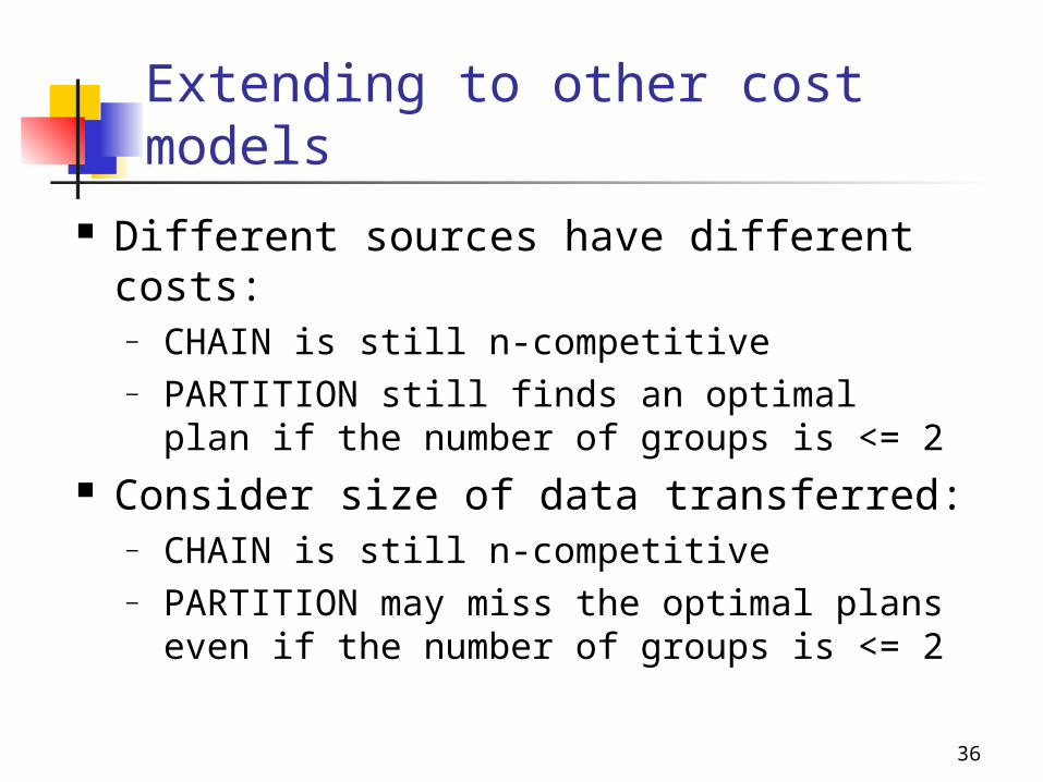
Extending to other cost models

Different sources have different costs:— CHAIN is still n-competitive— PARTITION still finds an optimal plan if

the number of groups is <= 2 Consider size of data transferred:

— CHAIN is still n-competitive— PARTITION may miss the optimal plans

even if the number of groups is <= 2

37

Given a query Q on relations with restrictions: Deciding whether all the answers to a query can be computed

Part II

38

Take Conjunctive queries (CQ’s) as an example

If the Inflationary algorithm terminates while some subgoals are not answerable, can we say there is no way to compute Q’s answers?— No!

Motivation

39

r(Star, Movie) s(Movie, Award)Harrison Ford Air Force One

Henry Fonda On Golden Pond

Kevin Spacey American Beauty

… …

On Golden Pond Oscar, Best Actor

On Golden Pond Oscar, Best Actress

American Beauty Oscar, Best Picture

… …

Example: A movie database

Q(Award) :- r(henry fonda,Movie), s(Movie,Award)

40

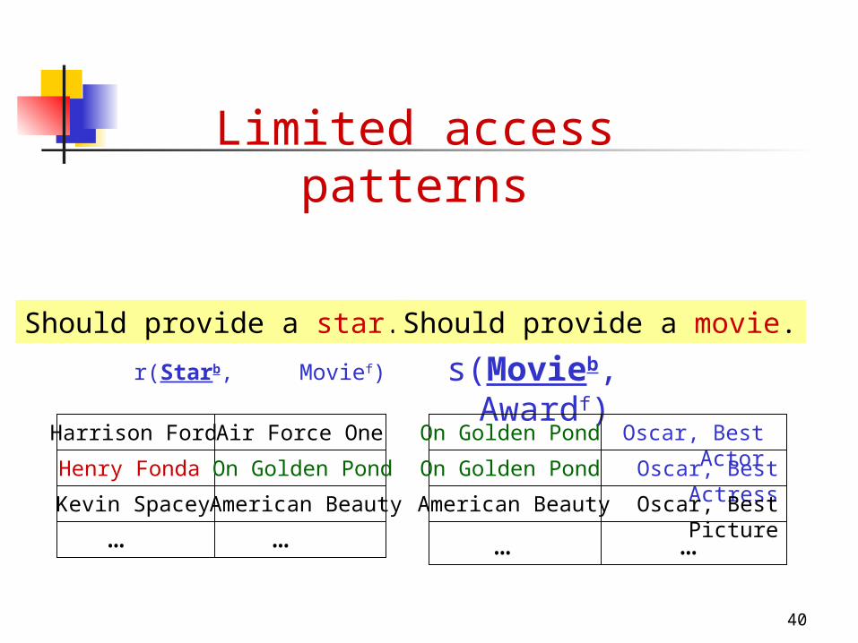
r(Starb, Movief) s(Movieb, Awardf)

Harrison Ford Air Force One



… …




… …

Limited access patterns

Should provide a star. Should provide a movie.

41




… …




… …

Answering Q given the restrictions



42




… …




… …

The answer is complete• We did not retrieve all the tuples from the relations.• Still we computed all tuples in the answer to the query.



43

Run Inflationary algorithm• Every subgoal would be answerable



44

How about Q’?

Q’(Award) :- r(henry fonda,Movie), s(Movie,Award),r(Star,Movie)

Inflationary will find that subgoal r(start,Movie) is not answerable

— variable Star cannot be bound Can we say Q’ cannot be answered?

— No!— It is essentially equivalent to the old query Q— Thus we can answer Q’ by answering Q!

45

Observations of binding patterns If a relation does not have an “all-free”

binding pattern, then after certain queries are sent to this relation, there can always be some tuples that have not been retrieved.

46

General questions Given a query on relations with

limited access patterns, can we compute its complete answer by accessing the relations with legal patterns? — If so, called “Stable” queries

The example shows that the solution is more than running the Inflationary algorithm

47

General questions (cont) Given a query Q, if Inflationary claims that

some subgoals are not answerable, how do we know whether there is another equivalent query Q’, such that Inflationary “succeeds” on Q’?

Notice that there are infinite number of equivalent queries of Q

Furthermore, even if Inflationary were able to say that all these equivalent queries have some unanswerable subgoal, how do we know if there isn’t any “magical” plan that can compute all the answers to Q?

48

Query stability A query Q on relations with binding

patterns is stable if for any database, we can compute its complete answer by accessing the relations with legal patterns.

The complete answer is the computable answer if we could retrieve all the tuples from the relations.

Use partial tuples to derive the complete answer: we need reasoning!

49

Feasible CQ’s A CQ is feasible if it has a feasible

(i.e., executable or answerable) order of all its subgoals.

Lemma: A feasible CQ is stable. Testing feasibility of a CQ:

Inflationary algorithm

50

What if Q is not feasible?

Our example shows that an infeasible query could still be stable

51

Testing stability of a CQ

Theorem: A CQ Q is stable iff its minimal equivalent Qm is feasible.

Minimal equivalent query Qm

Qm is unique

52

Main idea of the proof Construct two databases of the relations They have the same observable tuples, but

yield different answers to the query Thus, we cannot tell whether the computed

answer is complete or not

Same observable tuples

Database D1

Database D2

Different answers to Q

53

Another way to test CQ stability

Q: q(X) :- g1(),…, gk(), gk+1(), …, gn()

Q’: q(X) :- g1(),…, gk() Compute all executable (answerable)

subgoals of Q, wlog, denoted as g1(),…, gk() If all subgoals become executable, then Q is

stable Otherwise, test equivalence between Q and

Q’ Theorem: Q is stable iff Q and Q’ are

equivalent

54

Advantage of the second approach

Could be extended to other query classes— E.g., CQ’s with comparisons (“year >

1995”) Notice that in these classes,

“minimal equivalent query” of a query might not be unique or hard to find.

55

Two algorithms for testing stability of CQ’s

Algorithm CQStable— Minimize Q, get its minimal equivalent Qm

— Test feasibility of Qm by calling Inflationary

Algorithm CQStable*— Compute “executable” Q’ from Q— If all subgoals become executable, then Q is

stable— Otherwise, test equivalence between Q and Q’

CQStable* is more efficient than CQStable Testing stability of a CQ is NP-complete.

56

Other classes of queries Unions of CQs:

— Still we need to “minimize” the query first

— two algorithms for testing stability

57

CQs with arithmetic comparisons

More complicated due to potential equality among variables

Need to consider all total ordering An algorithm for the testing stability

58

Datalog queries Testing stability undecidable Give a sufficient condition for

stability of Datalog

59

Dynamic computability of complete answer to CQs

For a nonstable CQ Q, for certain database, its complete answer might be computed.

60

An exampleQ1: ans(B) :- r(a,B,C),s(C,D)

Not stable For the following database, we can still

compute Q1’s complete answer: {b1,b2}.

d1

d2

…

r(Ab, Bf, Cf)a b1

… …

c1

a b2 c2

a b2 c3

…

d1

…

c1

d2c2

…

s(Cf, Db) p(Df)

61

Change the head argumentQ2: ans(D) :- r(a,B,C),s(C,D)

Still not stable For the database, we cannot compute

Q2’s complete answer.

d1

d2

…

r(Ab, Bf, Cf)a b1

… …

c1

a b2 c2

a b2 c3

…

d1

…

c1

d2c2

…

s(Cf, Db) p(Df)

62

Difference between Q1 and Q2

b f f f b

Q1: ans(B) :- r(a,B,C),s(C,D)

Q2: ans(D) :- r(a,B,C),s(C,D) Q1’s head argument B is bound by

the executable subgoal r(a,B,C). Q2’s head argument D is not bound

by the executable subgoal r(a,B,C).

63

Generalizationq(X) :- g1(X1), …, gk(Xk),

gk+1(Xk+1), …, gn(Xn) Executable subgoals: E = g1(X1),…, gk(Xk) If all arguments in X are bound in E:

— we might compute its complete answer. — The computability is database dependent.

If some arguments in X are not bound in E:— we can never compute its complete answer. — Unless the relation after the subgoals in E is

empty.

64

A decision tree It guides the planning process of

computing the complete answer to a query.

Two approaches while traversing the tree:— optimistic— pessimistic

66

Conclusion We worked on research problems

on query processing and optimization in the presence of limited query capabilities

There are still research issues in this area

67

Peer-based distributed data integration and sharing

Data Cleansing to improve information quality

Other On-going research projects

68

Network

Peer User Interface W

rapper

Metadata Manager

Query Engine

Data Repository

Peer

Peer

Passive Source

User

User

Passive Source

User

Peer-based data integration and sharing

69

The RACCOON Project on Peer-based Data Integration and sharinghttp://www-db.ics.uci.edu/pages/raccoon/

70

The FLAMINGO PROJECT: CLEANSING DATA TO IMPROVE INFORMATION QUALITYhttp://www-db.ics.uci.edu/pages/flamingo/

1 query processing in the presence of limited source capabilities chen li information and computer...

Documents