1 probability and theoretical distributions. 2 since medicine is an inexact science, physicians...

1

PROBABILITY AND THEORETICAL

DISTRIBUTIONS

2

PROBABILITY AND THEORETICAL DISTRIBUTIONS

Since medicine is an inexact science, physicians seldom can predict an outcome with absolute certainty.

To formulate a diagnosis, a physician must rely on available diagnostic information about a patient (physical examinations or laboratory tests). If the test result is not absolutely accurate, decisions (diagnoses) relying on this result will be uncertain. Probability is a means for quantifying uncertainty.

3


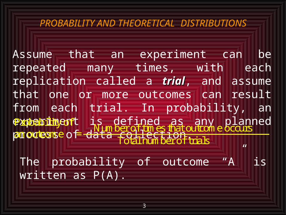
Assume that an experiment can be repeated many times, with each replication called a trialtrial, and assume that one or more outcomes can result from each trial. In probability, an experiment is defined as any planned process of data collection.

Number of times that outcome occurs Probability of an outcome =

Total number of trials

The probability of outcome “A” is written as P(A).

4


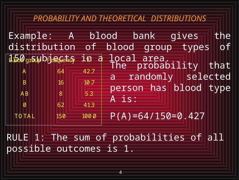
Example: A blood bank gives the distribution of blood group types of 150 subjects in a local area.

Blood group Frequency %

A 64 42.7

B 16 10.7

AB 8 5.3

0 62 41.3

TOTAL 150 100.0

The probability that a randomly selected person has blood type A is:

P(A)=64/150=0.427

RULE 1: The sum of probabilities of all possible outcomes is 1.

5


RULE 2: Two events are independent if the product of individual probabilities is equal to the probability that the two events happen together. In this case the outcome of one event, has no effect on the outcome of the other. If

P(A) * P(B) = P(A and B)

A and B are independent.

6


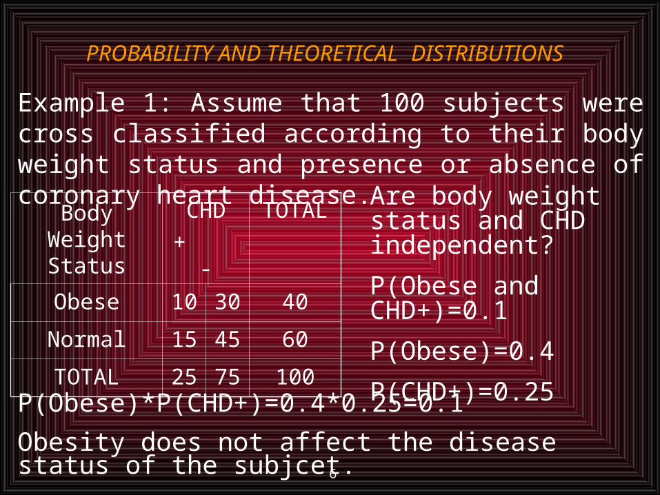
Example 1: Assume that 100 subjects were cross classified according to their body weight status and presence or absence of coronary heart disease.

Body Weight Status

CHD+ -

TOTAL

Obese 10 30 40

Normal 15 45 60

TOTAL 25 75 100

Are body weight status and CHD independent?

P(Obese and CHD+)=0.1

P(Obese)=0.4

P(CHD+)=0.25P(Obese)*P(CHD+)=0.4*0.25=0.1

Obesity does not affect the disease status of the subjcet.

7


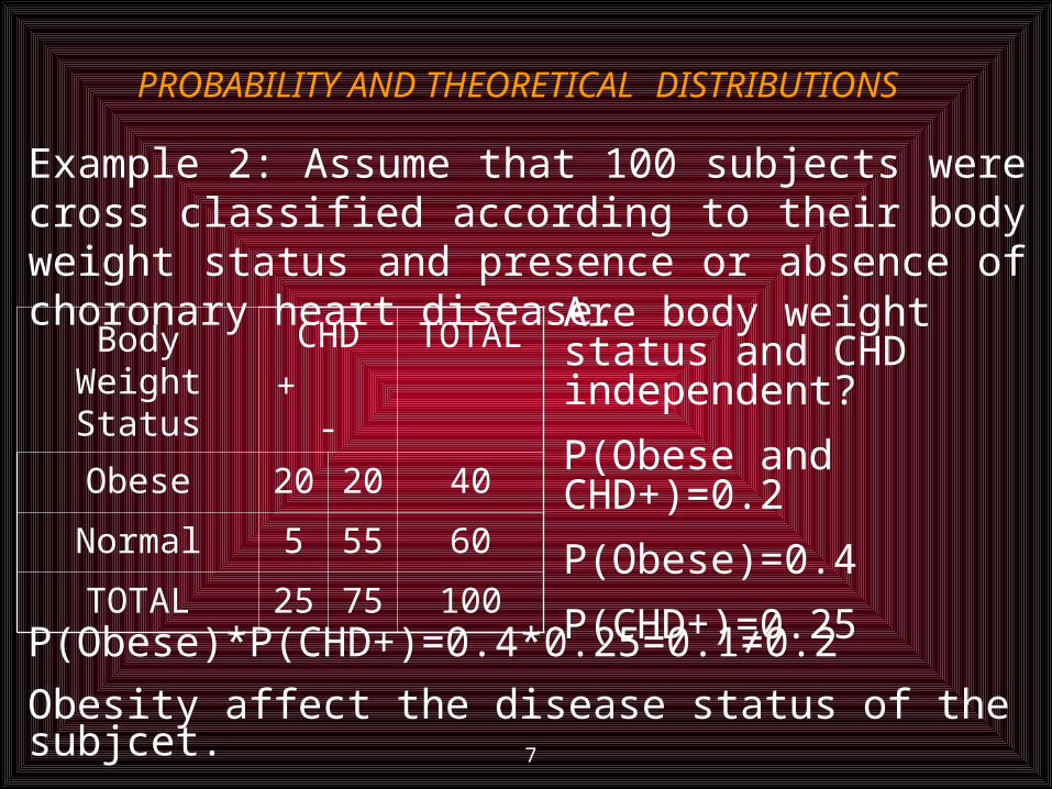
Example 2: Assume that 100 subjects were cross classified according to their body weight status and presence or absence of choronary heart disease.

Body Weight Status

CHD+ -

TOTAL

Obese 20 20 40

Normal 5 55 60

TOTAL 25 75 100

Are body weight status and CHD independent?

P(Obese and CHD+)=0.2

P(Obese)=0.4

P(CHD+)=0.25P(Obese)*P(CHD+)=0.4*0.25=0.1≠0.2

Obesity affect the disease status of the subjcet.

8


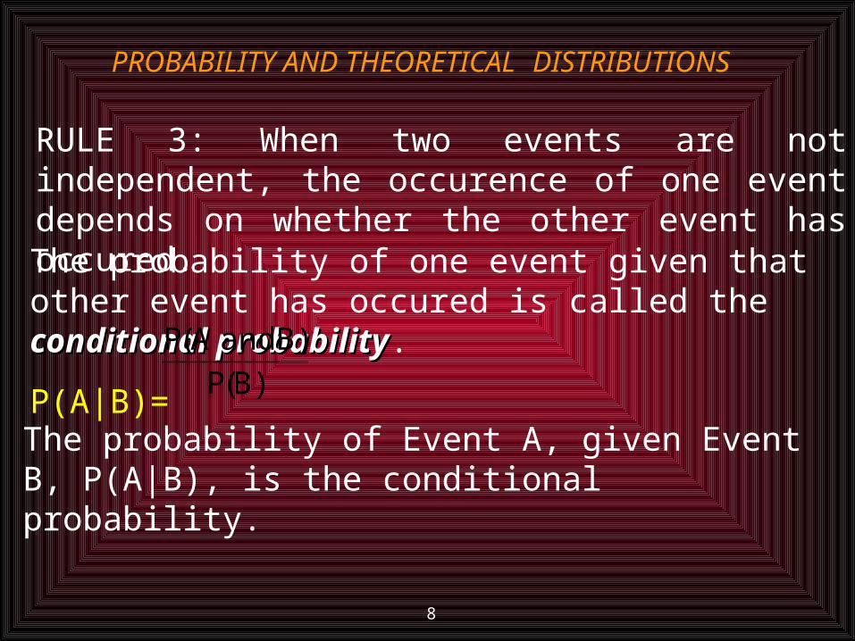
RULE 3: When two events are not independent, the occurence of one event depends on whether the other event has occured. The probability of one event given that other event has occured is called the conditional conditional probabilityprobability.

P(A|B)= )B(P)B and A(P

The probability of Event A, given Event B, P(A|B), is the conditional probability.

9


Body Weight Status

CHD+ -

TOTAL

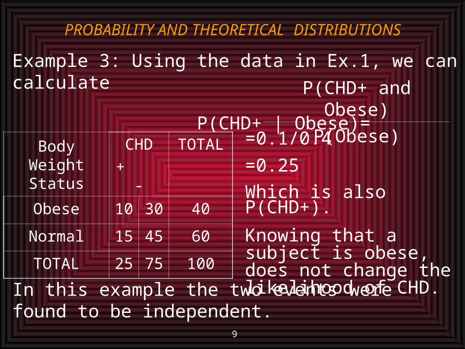
Obese 10 30 40

Normal 15 45 60

TOTAL 25 75 100

Example 3: Using the data in Ex.1, we can calculate

P(CHD+ | Obese)=

P(CHD+ and Obese)

P(Obese)=0.1/0.4

=0.25

Which is also P(CHD+).

Knowing that a subject is obese, does not change the likelihood of CHD.

In this example the two events were found to be independent.

10


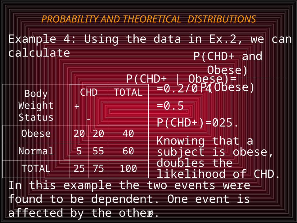
Body Weight Status

CHD+ -

TOTAL

Obese 20 20 40

Normal 5 55 60

TOTAL 25 75 100

Example 4: Using the data in Ex.2, we can calculate

P(CHD+ | Obese)=

P(CHD+ and Obese)

P(Obese)=0.2/0.4

=0.5

P(CHD+)=025.

Knowing that a subject is obese, doubles the likelihood of CHD.

In this example the two events were found to be dependent. One event is affected by the other.

11


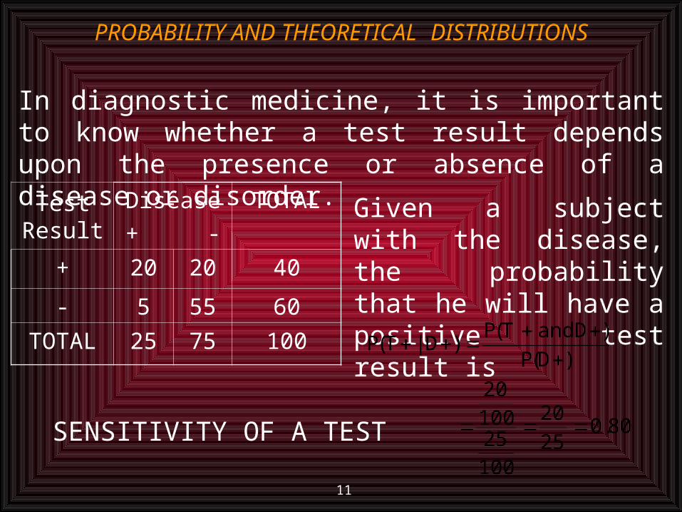
Test Result

Disease+ -

TOTAL

+ 20 20 40

- 5 55 60

TOTAL 25 75 100

In diagnostic medicine, it is important to know whether a test result depends upon the presence or absence of a disease or disorder.

Given a subject with the disease, the probability that he will have a positive test result is

80.02520

1002510020

)D(P)D andT(P

)D|T(P

SENSITIVITY OF A TEST

12


Test Result

Disease+ -

TOTAL

+ 20 20 40

- 5 55 60

TOTAL 25 75 100

Given a subject without the disease, the probability that he will have a negative test result is

73.07555

1007510055

)D(P)D andT(P

)D|T(P

SPECIFICITY OF A TEST

13


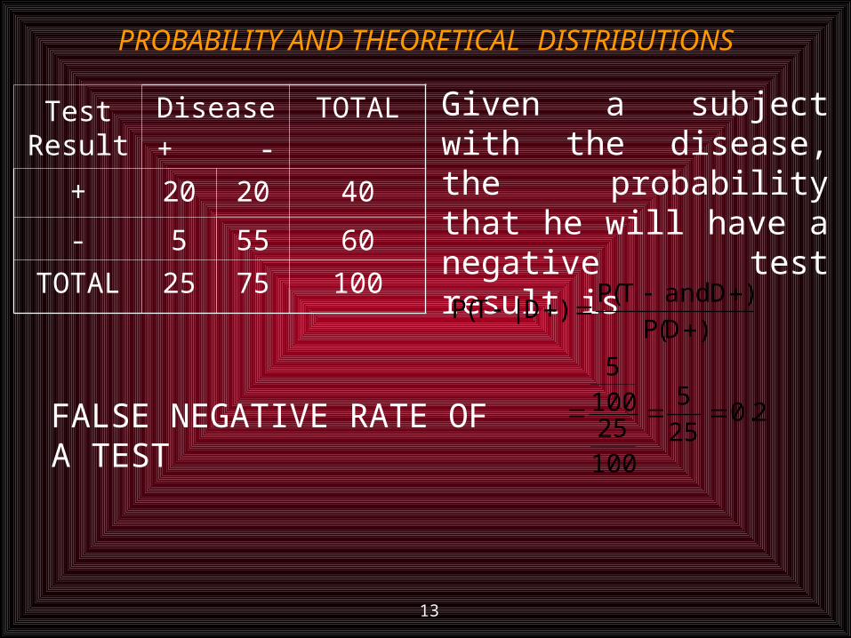
Test Result

Disease+ -

TOTAL

+ 20 20 40

- 5 55 60

TOTAL 25 75 100

Given a subject with the disease, the probability that he will have a negative test result is

2.0255

100251005

)D(P)D andT(P

)D|T(P

FALSE NEGATIVE RATE OF A TEST

14


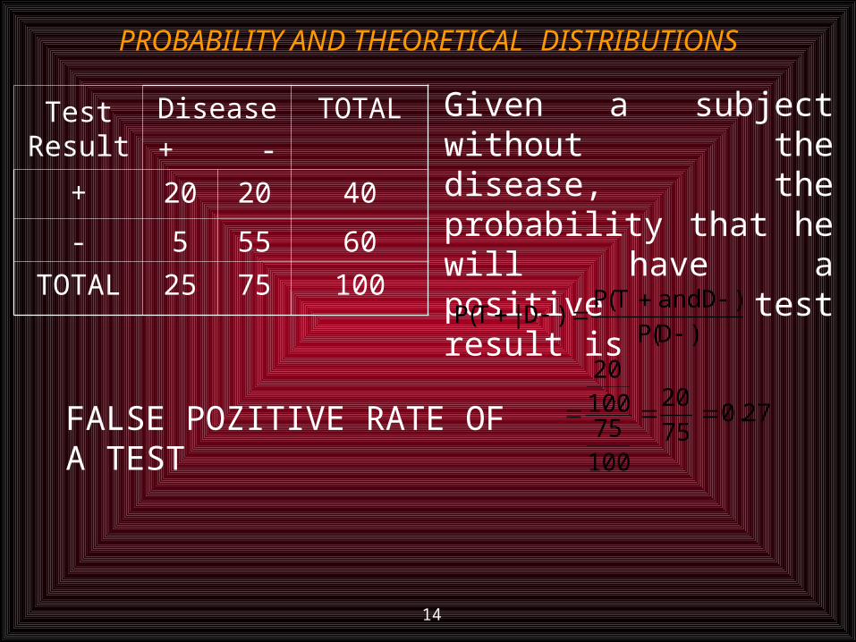
Test Result

Disease+ -

TOTAL

+ 20 20 40

- 5 55 60

TOTAL 25 75 100

Given a subject without the disease, the probability that he will have a positive test result is

27.07520

1007510020

)D(P)D andT(P

)D|T(P

FALSE POZITIVE RATE OF A TEST

15


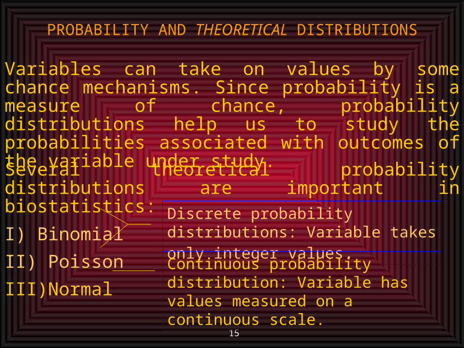
Variables can take on values by some chance mechanisms. Since probability is a measure of chance, probability distributions help us to study the probabilities associated with outcomes of the variable under study.

Several theoretical probability distributions are important in biostatistics:

I) Binomial

II) Poisson

III)Normal

Discrete probability distributions: Variable takes only integer values. Continuous probability distribution: Variable has values measured on a continuous scale.

16


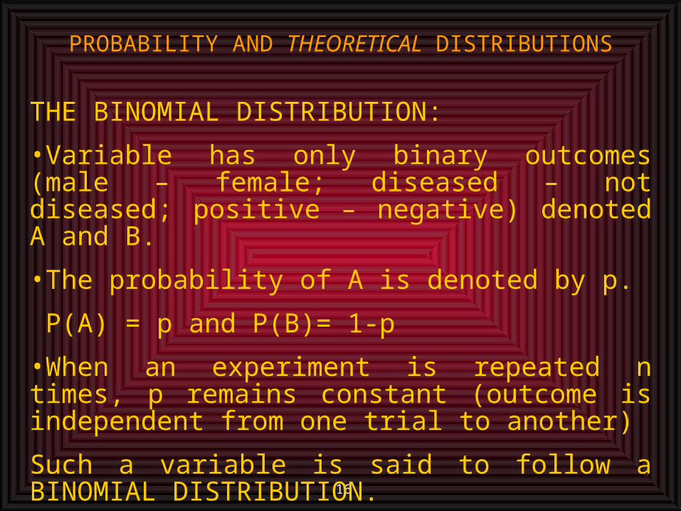
THE BINOMIAL DISTRIBUTION:

•Variable has only binary outcomes (male – female; diseased – not diseased; positive – negative) denoted A and B.

•The probability of A is denoted by p.

P(A) = p and P(B)= 1-p

•When an experiment is repeated n times, p remains constant (outcome is independent from one trial to another)

Such a variable is said to follow a BINOMIAL DISTRIBUTION.

17


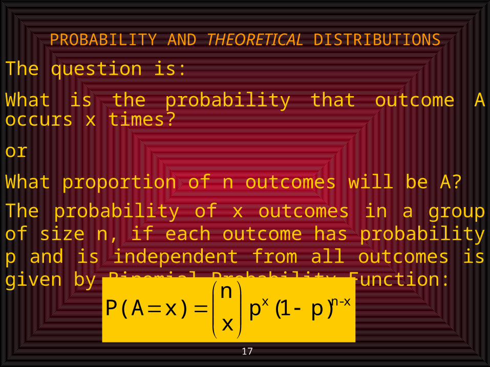
The question is:

What is the probability that outcome A occurs x times?

or

What proportion of n outcomes will be A?

The probability of x outcomes in a group of size n, if each outcome has probability p and is independent from all outcomes is given by Binomial Probability Function:

x-nx p)1(p x

nx)P(A

18


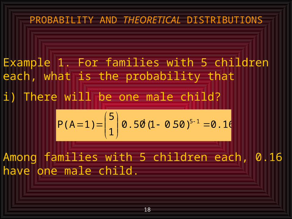
Example 1. For families with 5 children each, what is the probability that

i) There will be one male child?

0.16 )50.01(0.50 1

51)P(A 151

Among families with 5 children each, 0.16 have one male child.

19


ii) There will be at least one male children?

0.97

0.03- 1

0.5)-(1 0.5 0

5 -1

0)P(A-1

)5.01(0.5 A

5

5)P(A4)P(A3)P(A2)P(A1)P(A1)P(A

50

5

1A

A5A

20


Using the probabilities associated with possible outcomes, we can draw a probability distribution for the event under study:

NO. OF MALE CHILDREN

5,004,003,002,001,00,00

PR

OB

AB

ILIT

Y,4

,3

,2

,1

0,0

21


Example: Among men with localized prostate tumor and a PSA<10, the 5-year survival is known to be 0.8. We can use Binimial Distribution to calculate the probability that any particular number (A), out of n, will survive 5 years. For example for a new series of 6 such men:Non will survive 5 years : P(A=0)=0,000064Only 1 will survive 5 years : P(A=1)=0,00152 will survive 5 years : P(A=2)=0,0153 will survive 5 years : P(A=3)=0,0824 will sıurvive 5 years : P(A=4)=0,2465 will survive 5 years : P(A=5)=0,393All will survive 5 years : P(A=6)=0,262

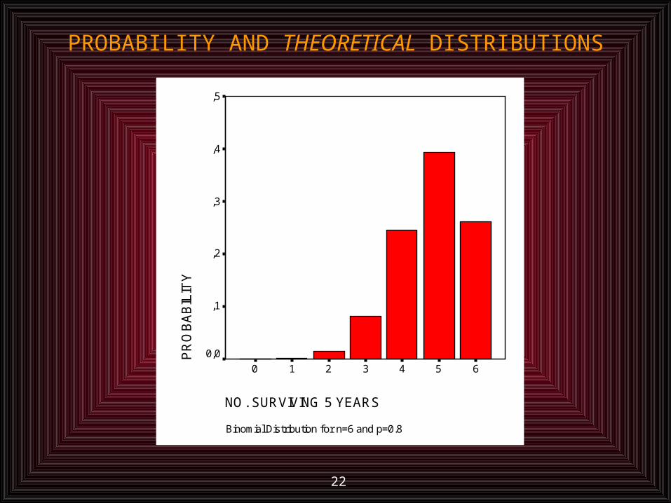
22

Binomial Distribution for n=6 and p=0.8

NO. SURVIVING 5 YEARS

6543210

PR

OB

AB

ILIT

Y

,5

,4

,3

,2

,1

0,0


23


THE POISSON DISTRIBUTION:

Like the Binomial, Poisson distribution is a discrete distribution applicable when the outcome is the number of times an event occurs. Instead of the probability of an outcome, if average number of occurence of the event is given, associated probabilities can be calculated by using the Poisson Distribution Function which is defined as:

!A

e)AX(P

A

24


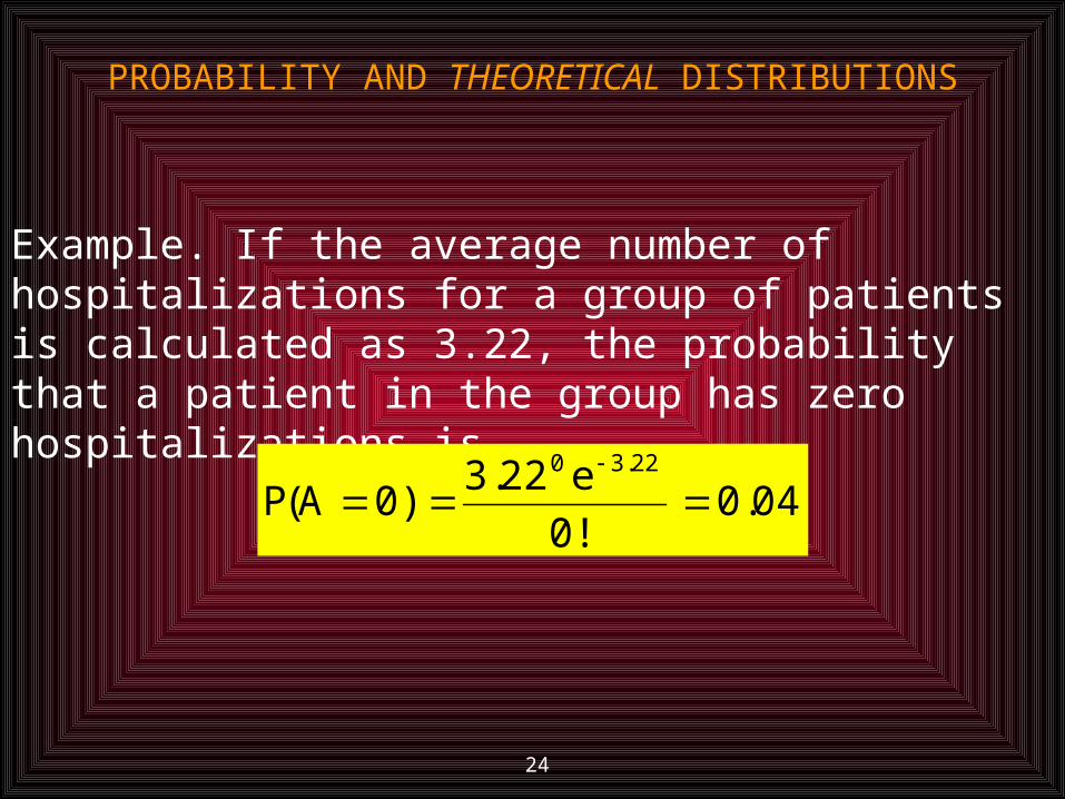
Example. If the average number of hospitalizations for a group of patients is calculated as 3.22, the probability that a patient in the group has zero hospitalizations is

04.0!0e22.3

)0A(P22.30

25


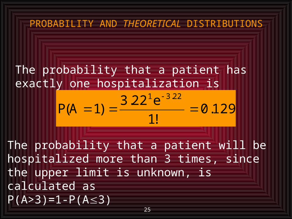
The probability that a patient has exactly one hospitalization is

129.0!1e22.3

)1A(P22.31

The probability that a patient will be hospitalized more than 3 times, since the upper limit is unknown, is calculated asP(A>3)=1-P(A3)

26

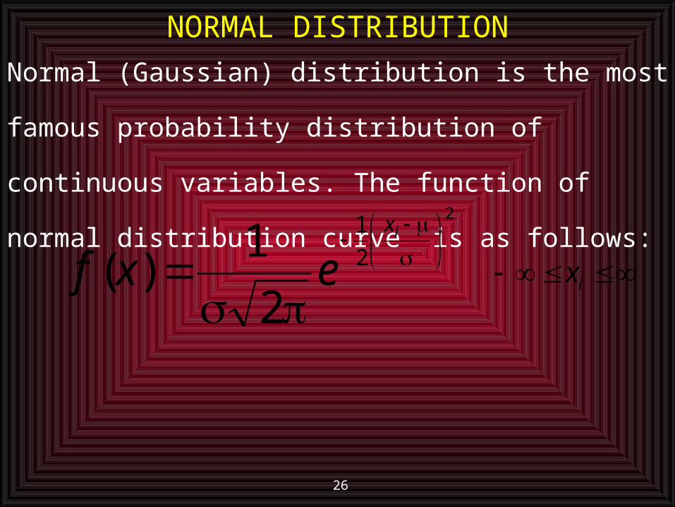
NORMAL DISTRIBUTION

Normal (Gaussian) distribution is the most

famous probability distribution of continuous

variables. The function of normal distribution

curve is as follows: ix

2

2

1

2

1)(

ix

exf

27

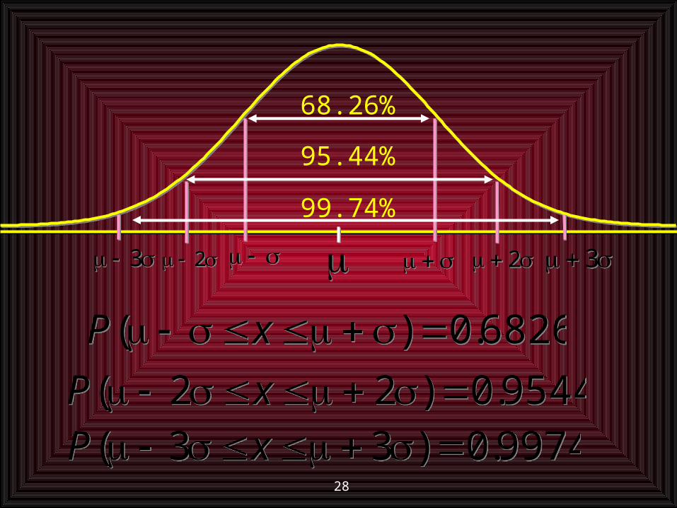
•It is a smooth, bell-shaped curve

•Half of the area is on the left of the mean and half the area is on the right.

•Sum of the probabilities for any given set of events is equal to 1.

µ

•It is symmetric around the mean of the distribution, symbolized by .

1)( dxxf

•Mean, median and mode are equal to the each other.

28

6826.0)( xP 6826.0)( xP

68.26%

9544.0)22( xP 9544.0)22( xP

2 2 2 2

95.44%

9974.0)33( xP 9974.0)33( xP

3 3 3 3

99.74%

29

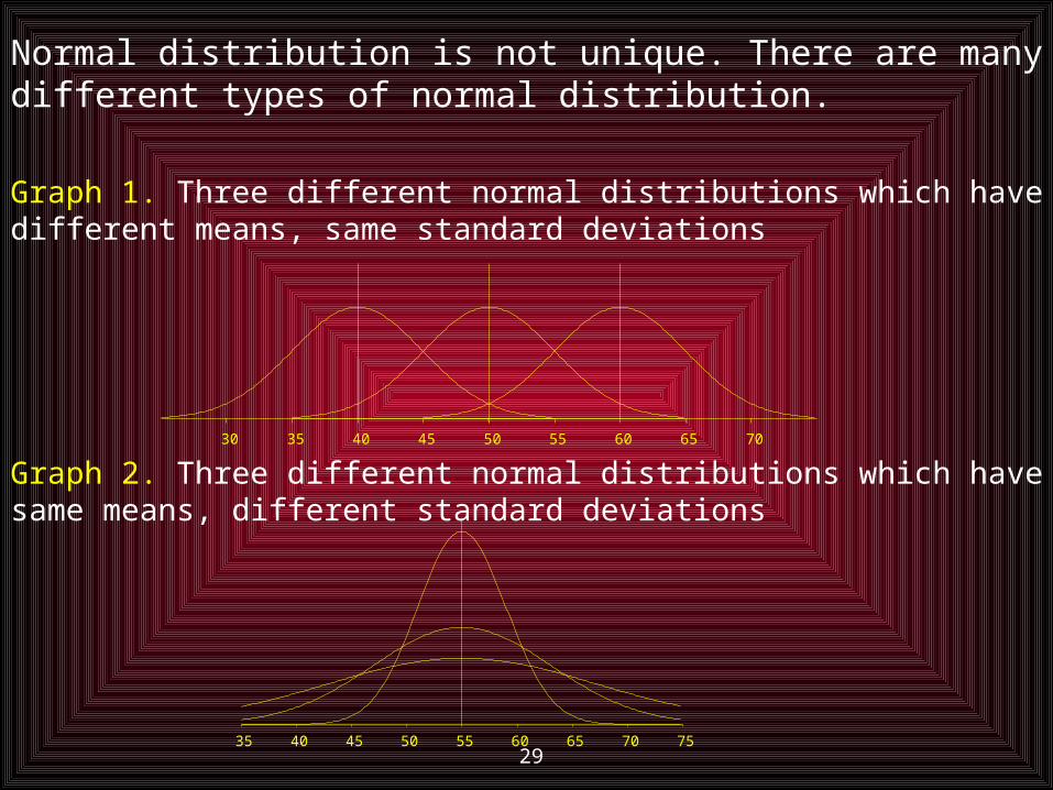
Normal distribution is not unique. There are many different types of normal distribution.

55 60 65 7035 40 45 5030

35 40 45 50 55 60 65 70 75

Graph 1. Three different normal distributions which have different means, same standard deviations

Graph 2. Three different normal distributions which have same means, different standard deviations

30

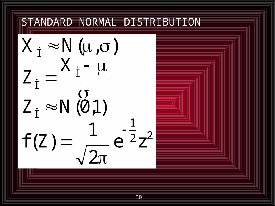
STANDARD NORMAL DISTRIBUTION

22

1İ

İİ

İ

ze2

1)Z(f

)1,0(NZ

XZ

),(NX

31

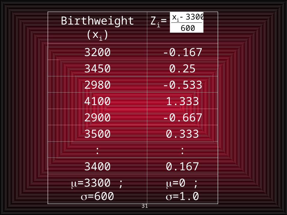
Birthweight (xi) Zi=

3200 -0.167

3450 0.25

2980 -0.533

4100 1.333

2900 -0.667

3500 0.333

: :

3400 0.167

=3300 ; =600 =0 ; =1.0

600

3300x i

32

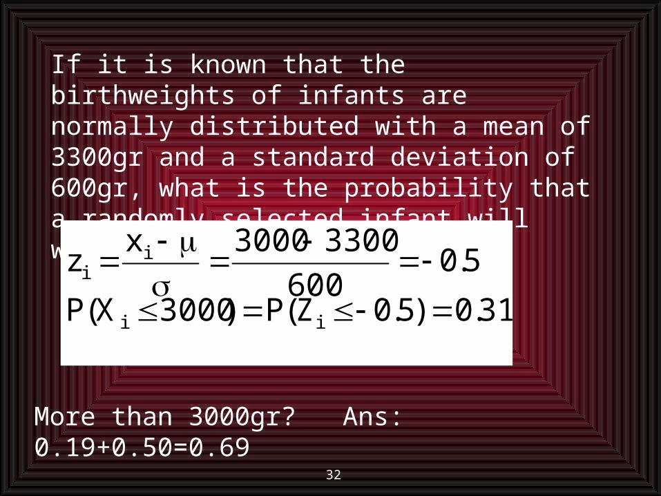
If it is known that the birthweights of infants are normally distributed with a mean of 3300gr and a standard deviation of 600gr, what is the probability that a randomly selected infant will weigh less than 3000gr?

31.0)5.0Z(P)3000X(P

5.0600

33003000xz

ii

ii

More than 3000gr? Ans: 0.19+0.50=0.69

33

0.00 0.01 0.02 0.03 0.04 0.05 0.06 0.07 0.08 0.09

0.0 0.0000 0.0040 0.0080 0.0120 0.0160 0.0199 0.0239 0.0279 0.0319 0.0359

0.1 0.0398 0.0438 0.0478 0.0517 0.0557 0.0596 0.0636 0.0675 0.0714 0.0753

0.2 0.0793 0.0832 0.0871 0.0910 0.0948 0.0987 0.1026 0.1064 0.1103 0.1141

0.3 0.1179 0.1217 0.1255 0.1293 0.1331 0.1368 0.1406 0.1443 0.1480 0.1517

0.4 0.1554 0.1591 0.1628 0.1664 0.1700 0.1736 0.1772 0.1808 0.1844 0.1879

0.5 0.1915 0.1950 0.1985 0.2019 0.2054 0.2088 0.2123 0.2157 0.2190 0.2224

0.6 0.2257 0.2291 0.2324 0.2357 0.2389 0.2422 0.2454 0.2486 0.2517 0.2549

0.7 0.2580 0.2611 0.2642 0.2673 0.2704 0.2734 0.2764 0.2794 0.2823 0.2852

0.8 0.2881 0.2910 0.2939 0.2967 0.2995 0.3023 0.3051 0.3078 0.3106 0.3133

0.9 0.3159 0.3186 0.3212 0.3238 0.3264 0.3289 0.3315 0.3340 0.3365 0.3389

1.0 0.3413 0.3438 0.3461 0.3485 0.3508 0.3531 0.3554 0.3577 0.3599 0.3621

1.1 0.3643 0.3665 0.3686 0.3708 0.3729 0.3749 0.3770 0.3790 0.3810 0.3830

1.2 0.3849 0.3869 0.3888 0.3907 0.3925 0.3944 0.3962 0.3980 0.3997 0.4015

1.3 0.4032 0.4049 0.4066 0.4082 0.4099 0.4115 0.4131 0.4147 0.4162 0.4177

1.4 0.4192 0.4207 0.4222 0.4236 0.4251 0.4265 0.4279 0.4292 0.4306 0.4319

1.5 0.4332 0.4345 0.4357 0.4370 0.4382 0.4394 0.4406 0.4418 0.4429 0.4441

1.6 0.4452 0.4463 0.4474 0.4484 0.4495 0.4505 0.4515 0.4525 0.4535 0.4545

1.7 0.4554 0.4564 0.4573 0.4582 0.4591 0.4599 0.4608 0.4616 0.4625 0.4633

1.8 0.4641 0.4649 0.4656 0.4664 0.4671 0.4678 0.4686 0.4693 0.4699 0.4706

1.9 0.4713 0.4719 0.4726 0.4732 0.4738 0.4744 0.4750 0.4756 0.4761 0.4767

2.0 0.4772 0.4778 0.4783 0.4788 0.4793 0.4798 0.4803 0.4808 0.4812 0.4817

2.1 0.4821 0.4826 0.4830 0.4834 0.4838 0.4842 0.4846 0.4850 0.4854 0.4857

2.2 0.4861 0.4864 0.4868 0.4871 0.4875 0.4878 0.4881 0.4884 0.4887 0.4890

2.3 0.4893 0.4896 0.4898 0.4901 0.4904 0.4906 0.4909 0.4911 0.4913 0.4916

2.4 0.4918 0.4920 0.4922 0.4925 0.4927 0.4929 0.4931 0.4932 0.4934 0.4936

2.5 0.4938 0.4940 0.4941 0.4943 0.4945 0.4946 0.4948 0.4949 0.4951 0.4952

2.6 0.4953 0.4955 0.4956 0.4957 0.4959 0.4960 0.4961 0.4962 0.4963 0.4964

2.7 0.4965 0.4966 0.4967 0.4968 0.4969 0.4970 0.4971 0.4972 0.4973 0.4974

2.8 0.4974 0.4975 0.4976 0.4977 0.4977 0.4978 0.4979 0.4979 0.4980 0.4981

2.9 0.4981 0.4982 0.4982 0.4983 0.4984 0.4984 0.4985 0.4985 0.4986 0.4986

3.0 0.4987 0.4987 0.4987 0.4988 0.4988 0.4989 0.4989 0.4989 0.4990 0.4990

Area between 0 and z

34

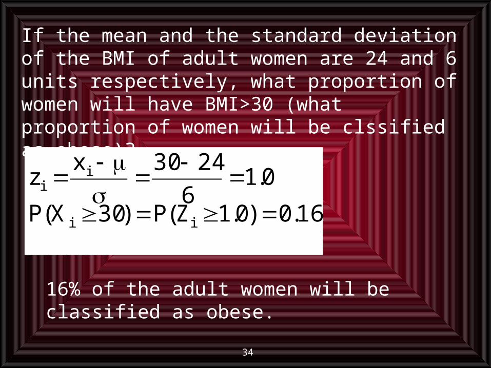
If the mean and the standard deviation of the BMI of adult women are 24 and 6 units respectively, what proportion of women will have BMI>30 (what proportion of women will be clssified as obese)?

16.0)0.1Z(P)30X(P

0.16

2430xz

ii

ii

16% of the adult women will be classified as obese.

35

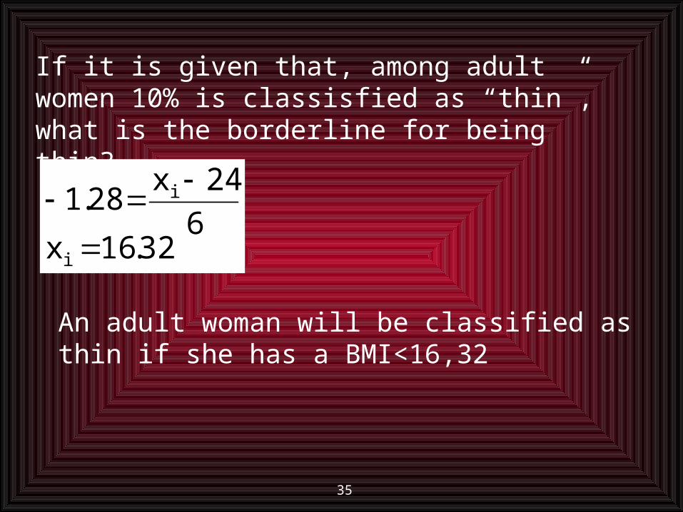
If it is given that, among adult women 10% is classisfied as “thin”, what is the borderline for being thin?

32.16x6

24x28.1

i

i

An adult woman will be classified as thin if she has a BMI<16,32

1 probability and theoretical distributions. 2 since medicine is an inexact science, physicians...

Documents