-1- potential applications of magnetic gradients …
TRANSCRIPT

-1-
POTENTIAL APPLICATIONS OF MAGNETIC GRADIENTS
TO MARINE GEOPHYSICS
by
WILLIAM E. BYRD, JR.
S.B., Massachusetts Institute of Technology
Submitted in Partial Fulfillment
of the Requirements for the
Degree of Master of Science
at the
MASSACHUSETTS INSTITUTE OF TECHNOLOGY
June, 1967
Signature of Author
Certirea by
Department of Geology ad Geophysics
Thesis Supervisor
Accepted by
Chairman, Departmental Committee
on Graduate Students
-2-
POTENTIAL APPLICATIONS OF MAGNETIC GRADIENTS TO MARINE GEOPHYSICS
by
WILLIAM E. BYRD
Submitted tothe Department of Geology and Geophysics
on June 1967in partial fulfillment of the requirement
for the degree of Master of Science
Magnetic gradients offer numerous advantages over total magnetic fieldintensity when used for geological and geophysical interpretation.
1. Horizontal variations of the gradients emphasize the short wavelengthspatial components of magnetic anomalies.
2. Anomalies arising from near sources are enhanced over those arisingfrom deeper or more distant sources.
3. Long wavelength spatial components associated with regional trendsand large scale anomalies are attenuated.
4. Gradient observations made by differential measurement techniquesare unaffected by field intensity variations in time (diurnal shifts, secularchanges, magnetic storms, micropulsations, etc.).
5. Gradient data contain an inherent zero reference and need not bereduced to residual anomaly data.
Chapter I is a consideration of application of magnetic gradients to---marine geophysics and it shows that gradients are well-suited to the investi-gation of sea floor structure. Gradients may be utilized in the followingareas of study:
1. investigation of magnetic anomaly fine structure;2. delineation of geologic contact position and orientation;3. estimation of depth to source and source type; and4. determination of magnetization direction from topographic effects.This chapter also discusses the requirements for a marine magnetic
gradiometer and proposes a system utilizing two Zeeman sensors in a stablevertical towed array. It also includes investigation of error sources andmeans for their correction or reduction.
Chapter II reviews present knowledge and theory of ocean ridge structure,with emphasis on the characteristic magnetic anomalies observed over theridges. We propose that these anomalies arise from a sub-horizontal laye restructure composed of basaltic flows which have originated in the ridge's axial
region. Included in this presentation is a sub-horizontal layered model of theReykjanes Ridge. Computed magnetic anomaly profiles over this model correlatewell with observed profiles taken from a survey by Heirtzler.
Magnetic gradients offer a means to test the validity of the sub-
horizontal layered hypothesis of mid-ocean ridge structure. We propose the
use of magnetic gradients to determine the position and orientation of
geologic contacts in the ridge structure. Spcifica ly, the gradients can
be used to determine the general dip of contacts between regions of different
magnetic characteristics. If these dips are small, the sub-horizontal
layered hypothesis is justified.
Thesis Supervisor: David W. StrangwayTitle: Assistant Professor of Geophysics

-3-
Acknowledgments
The author's interest in magnetic gradients and their application to
marine geophysics was stimulated and encouraged by discussions with
Drs. R. P. Von Herzen and J. D. Phillips of the Woods Hole Oceanographic
Institution. Professor F. Press, Head of the Department of Geology and
Geophysics, Massachusetts Institute of Technology, offered further
encouragement and advice. The author is grateful for the direction and
assistance provided by Professor D. W. Strangway.
Model computations were performed with the aid of the Fortran Monitor
System and IBM 7094 of the MIT Computation Center.
The author is particularly indebted to L. B. S. Sloan, whose persistence
and expertise as editor and typist in the preparation of this report made
its writing much easier than it might otherwise have been.
-4-
Table of Contents
page
I. APPLICATION OF MARINE GRADIENTS 7TO MARINE GEOPHYSICS
Introduction 8
The Earth's Magnetic Field 9
Marine Magnetics 10
The Question of Resolution 15
Magnetic Gradient Theory 18
Gradients Over Geologic Contacts 21
Gradients Over Single Pole and Dipole Sources 30
Gradients and Topography 32
Computer Models 33
A Marine Gradiometer System 43
Gradient Error Sources 50
References 56

Table of Contents
page
II. A PROPOSED INVESTIGATION 59OF MID-OCEAN RIDGE STRUCTURE
Mid-Ocean Ridges and their Geologic Structure 60
Vertical versus Horizontal Structure 63
The Reyjkanes Ridge Model 66
Logic of the Horizontal Structure 71
Methods for the Study of Ocean Ridge Structure 73
Magnetic Field Gradients 75
Magnetic Gradients and Ocean Ridge Structure 85
Conclusion 87
References 89
Appendix 1A PROGRAM FOR COMPUTATION AND PLOTTING 91OF MAGNETIC ANOMALIES AND GRADIENTSOVER TWO-DIMENSIONAL POLYCGONS OF IRREGULAR CROSS-SECTION
Appendix 2ADDITIONAL COMPUTER MODELS 114
Biography 133

List of Illustrations
page
I. APPLICATION OF MARINE GRADIENTSTO MARINE GEOPHYSICS
Fig. 1: Geologic Contact Geometry 23Fig. 2: Gradients over Dipping Contact; a = 450 24Fig. 3: Vertical Gradients over Block Model 34
Fig. 4: Vertical Gradients over Topography 35Fig. 5: Horizontal Gradients over Topography 36Fig. 6: Vertical Gradients over Model No. 8 38
Fig. 7: Horizontal Gradients over Model No. 8 39Fig. 8: Vertical Gradients over Horizontal-Layered Model 40
Fig. 9: Horizontal Gradients over Horizontal-Layered Model 41
Fig. 10 Horizontal Gradients over Model No. 12 42
Fig.11: Maximum Vertical Gradient 45Over a Steeply-Dipping Geologic Contact
Fig. 12: A Proposed Marine Gradiometer System 47
Fig. 13: Rubidium Sensor Orientation 54
II. A PROPOSED INVESTIGATIONOF MID-OCEAN RIDGE STRUCTURE
Fig. 1: The Reykjanes Ridge Model 67
Fig. 2: Observed and Calculated Anomalies 70Over the Reykjanes Ridge
Fig. 3: Geologic Contact Geometry 79Fig. 4: Gradients over Dipping Contact; a = 45 80Fig. 5: Gradients over Vertical Structure 83
Fig. 6: Gradients over Horizontal Structure 84
-7-
I. APPLICATION OF MAGNETIC GRADIENTS
TO MARINE GEOPHYSICS

-8-
Introduction
The history of marine magnetics is brief. Recognition of the existence
of a magnetic field associated with the earth was apparently first made by
Gilbert (c. 1540--1603) in his pioneer studies of magnetism described in
De Magnete, published in 1600. Thecompass had, of course, been widely known
and used for several thousand years. The earliest investigations of the
earth's field sought to map declination and dip in order to make the compass
a reliable instrument of navigation. Later, as instruments became more
sophisticated, investigators began to study the variations with time and
location of the horizontal and vertical field components. It was not until
the late 1940's and 50's, after the military development of sensitive and
accurate portable magnetometers for submarine detection, that magnetic field
data taken at sea could be collected routinely and combined with other
geophysical data. This combination of seismic, gravimetric and magnetic
data forms the basis of marine geophysics which today strives to increase
our knowledge of the composition, structures and physical processes of the
sea floor. Due to inherent instrument limitations and the difficulties of
working from a ship it has been most convenient and common to make
measurements only of total magnetic field intensity.
-9-
The Earth's Magnetic Field
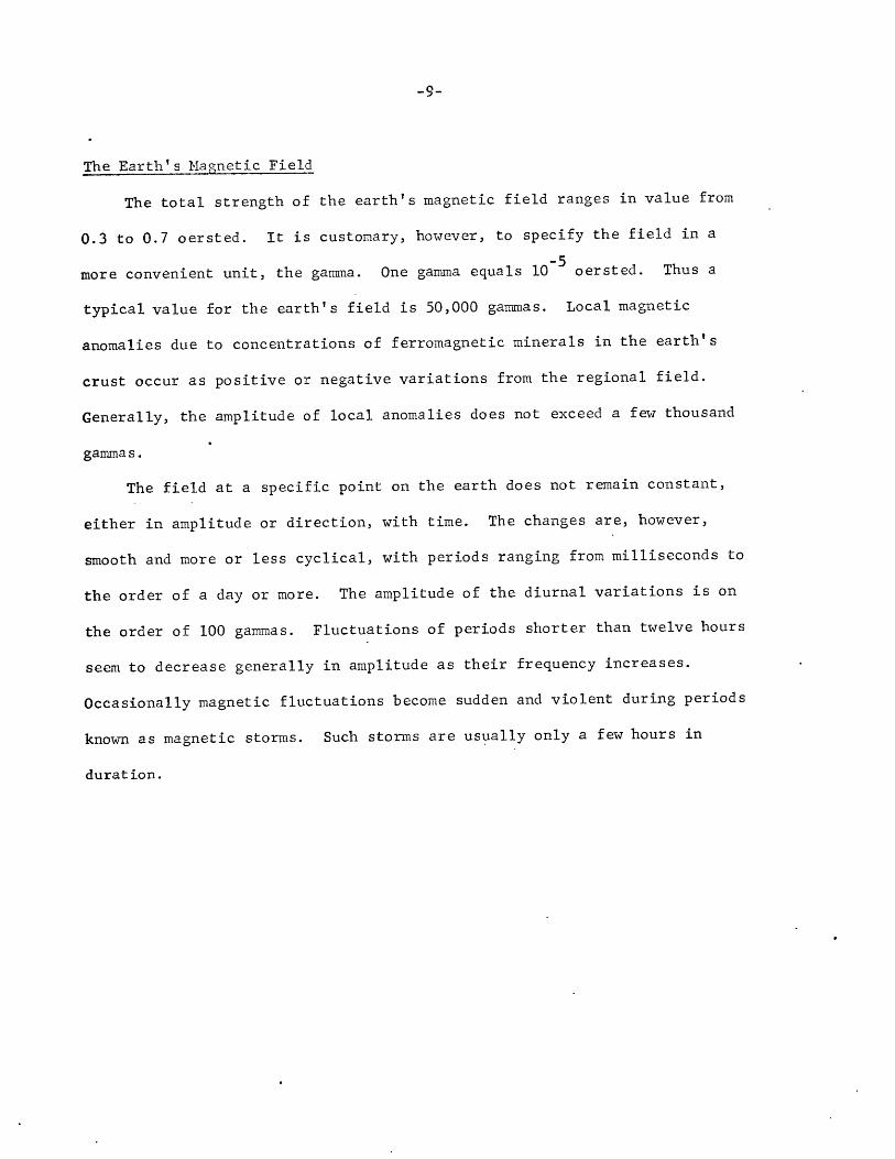
The total strength of the earth's magnetic field ranges in value from
0.3 to 0.7 oersted. It is customary, however, to specify the field in a-5
more convenient unit, the gamma. One gamma equals 10-5 oersted. Thus a
typical value for the earth's field is 50,000 gammas. Local magnetic
anomalies due to concentrations of ferromagnetic minerals in the earth's
crust occur as positive or negative variations from the regional field.
Generally, the amplitude of local anomalies does not exceed a few thousand
gammas.
The field at a specific point on the earth does not remain constant,
either in amplitude or direction, with time. The changes are, however,
smooth and more or less cyclical, with periods ranging from milliseconds to
the order of a day or more. The amplitude of the diurnal variations is on
the order of 100 gammas. Fluctuations of periods shorter than twelve hours
seem to decrease generally in amplitude as their frequency increases.
Occasionally magnetic fluctuations become sudden and violent during periods
known as magnetic storms. Such storms are usually only a few hours in
duration.
-10-
Marine Magnetics
Total field magnetometers suitable for ship operation are of three
basic types: the fluxgate, the proton-procession, and the optically-pumped
Zeeman effect. Their sensitivities and characteristics are shown in Table 1.
The Varian rubidium vapor magnetometer is an example of the Zeeman effect
type. To date the rubidium vapor magnetometer has not been used for
survey-type operations at sea. Its extreme sensitivity is in fact a liability
unless the instrument can be accurately and stably positioned and operated
in a mode which distinguishes temporal from spatial variations in field
intensity. A ship is neither stable, nor is its position well-known, and
the standard method of compensating for temporal fluctuations with base
station observations is impractical, if not impossible, at sea.
The magnetic field, unlike the gravitational field, is dipolar, and so
long as the distance, r, of the observer from the dipole is great compared
to the dipole separation, the magnetic field intensity is proportional to
1/r 3 . Magnetic anomalies are usually attributed to a geologic dipole source,
such as a spherical or lenticular body, or a series of dipoles arranged side
by side to form a vein, fault, or dike. In addition to the 1/r 3 loss in
amplitu-es, the apparent dimensions of a sharp ainomaly are increa?d
greater distances due to greater attenuation of higher frequency components.
These facts lead us to the conclusion that, in order to study the
details of geologic structure, magnetic measurements must be made as close
to the source of the anomaly as possible. In the case of oceanic surveys,
we certainly cannot expect high resolution from measurements made at the sea
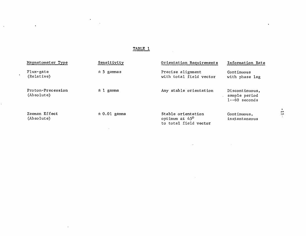
TABLE 1
Magnetometer Type
Flux-gate(Relative)
Proton-Precession(Ab so lute)
Zeeman Effect(Absolute)
Sensitivity
± 5 gammas
S1 gamma
± 0.01 gamma
Orientation Requirements
Precise alignmentwith total field vector
Any stable orientation
Stable orientationoptimum at 450to total field vector
Information Rate
Continuouswith phase lag
Discontinuous,sample period1--60 seconds
Continuous,instantaneous

-12-
surface when the geological structures responsible for the anomalies lie
4 kilometers or more below. This is analogous to performing an aeromagnetic
survey from 12,000 feet. The obvious solution to this problem is to place
the magnetometer closer to the sea floor, either in a submarine vehicle, or
as a deep-towed system operated from a surface ship. The technology of
deep submersibles, manned or unmanned, is not sufficiently advanced to allow
their use as vehicles for extended magnetic surveys. The problems of depth
capability, endurance, cost, speed and navigation all bar the way to
effective and extensive use of submarine vehicles for scientific activity.
The concept of a deep-towed magnetometer is not new. The Thresher
search (1963) demonstrated the need for a system capable of producing a
high-resolution magnetic survey in a deep-ocean area. During the search
several deep-towed magnetometer systems were quickly built and work has
continued on deep-towed magnetometers at the Naval Research Laboratory,
Scripps Institution of Oceanography, and Lamont Geological Observatory.
However, such a system is beset by certain basic problems and limitations.
The greatest of these is naviagation. In this case the problem is compounded,
since it is not the ship's position which must be known but that of the
magnetometer itself, whica may be at the end of fiv-, miles or more of
flexible cable. In practice it is necessary to monitor continuously the
actual position, horizontal and vertical, of any deep-towed system. This
is usually done by acoustic triangulation, either from a surface baseline
established by hydrophones towed astern and to either side of the surface
ship, or by a transponder system utilizing units accurately positioned on

-13-
the ocean floor. Either method requires expensive and complicated
equipment as well as computer data reduction.
By experience, the practical limit on speed, when towing to depths
greater than 4 kilometers, has been found to be around two knots. Beyond
this speed, stress at the tow point approaches the working strength of
available cable materials and the scope-to-depth ratio becomes impractical,
introducing even greater complications into the navigation problem.
The low ship speeds at which a deep-towed system must be operated lead
to important considerations of ship time and cost, especially in the case of
survey-type operations where the total ship track may be extremely long.
For example, a magnetic survey conducted in middle latitudes with a 5
nautical mile grid spacing would require approximately 1,000 nautical miles
of ship track to cover a one-degree square. Travelling at 2 knots, this
would require twenty days of ship time. Since the operating costs of an
appropriate ship are $2,000 to $4,000 per day, one might well ask whether
the high cost, in money and time, of operating a deep-towed system is
justified.
Over-land aeromagnetic surveys are commonly utilized to cover large
areas The acromagneti, survey is quick and the Cu-t per line m'ilc ic
small. Marine aeromagnetic surveys have been attempted (Heirtzler et al
(1966)). However, there are several difficulties which make the marine
aeromagnetic survey generally unsuited to precise, high resolution work.
Ground control, normally furnished by aerial photography, is non-existent,
and precision navigation is usually unavailable. Due to the lack of position
-14-
control it is therefore difficult to tie magnetic data in with other
geophysical information gathered usually by ships at a different time and
with equally loose position control. For these reasons, marine aeromagnetic
surveys are most useful in delineating large scale regional anomalies and
trends.
-15-
The Question of Resolution
Marine magnetic surveys conducted from the sea surface are
resolution limited. The deep-towed magnetometer is one approach toward
improved resolution which will enable us to study the "fine structure" of
known magnetic anomali >;. It is important to remember that when we speak
of resolution, we are concerned with the spatial frequency components of the
magnetic record as well as amplitude variation in total field strength.
In practice, the high-frequency components are generally of low amplitude,
so that the problem of improving resolution is a two-fold one of frequency
response and sensitivity. The surface-towed proton-precession magnetometer
is in an inherently poor position to provide high-resolution data. First,
its sensitivity is only one gamma. Second, it is not a continuous
recording instrument; having instead an operating cycle with a variable
sample period of 1 to 60 seconds. This imposes a limit on frequency
response, since the highest frequency appearing in the record cannot have
a period greater than twice that of the sample period. For a sample period
of 30 seconds and a ship speed of 15 knots, the shortest wavelength in
the record would be 0.5 kilometer. The shortest wavelength discernible by
visual " spection from sdch a record wou"' probably ui va the orC -r c
2 or 3 kilometers. In addition, since the closest possible source of
anomalies, the ocean floor, lies 4 or 5 kilometers beneath the magnetometer,
the attenuation of short wavelength components is extremely great for
wavelengths of the same order of magnitude as the water depth. If anomalies
are represented by a space spectrum, a component of wavelength % will be
-165-
reduced in the ratio exp (-2jz/) if it is measured at a distance z above
the bottom. In water of 5,000 meters depth the attenuation is by a factor
of 2 for all wavelengths less than 14 km. Since shorter wavelength anomalies
in general have initially lower amplitudes, this increasing attenuation of
short wavelength components results in a very substantial loss of detail at
the sea surface.
The limitations of the proton precession magnetometer are overcome by
the rubidium vapor magnetometer which has a sensitivity of 0.01 gamma, two
orders of magnitude better, and which is a continuously recording instrument.
But increased sensitivity, by itself, is not the answer to the problem of
higher resolution. The exponential attenuation of short wavelength
components is the most important single factor affecting resolution. In
fact, if the rubidium vapor magnetometer were used at sea as a total field
strength instrument, we might expect its high sensitivity to be as much a
liability as an asset. Errors due to the proximity of the ship and unwanted
motions of the sensor, which at lower sensitivities have been negligible,
could no longer be ignored. Temporal fluctuations in field strength would
continue to be indistinguishable from spatial variations due to geologic
structures without the aid of base station obsrvrtions And most
important, temporal fluctuations in the frequency region of greatest
interest, that is those frequencies corresponding to the short wavelength
components of geologic or topographic structures, would dominate the
attenuated spatial variations.
All of the limitations discussed above are greatly reduced or eliminated

-17-
if instead of total field strength we measure magnetic gradients and observe
their horizontal variations.
/
-18-
Magnetic Gradient Theory
We will now develop the theory which will enable us to utilize gradients
in magnetic interpretation. We shall find that the gradients are especially
useful in marine geomagnetics. We must remember, however, that the gradients
add no new information beyond that contained within total field intensity
measurements. The ambiguities inherently present in any interpretation
based on potential field theory remain. None of the geologic variables are
eliminated by the use of gradients. Assumptions are still necessary and
solutions in most cases are still non-unique. The value of gradients lies
in their ability to eliminate the magnetic effects arising from non-geologic
sources, and in their use as a high resolution tool for study of the fine
structure of magnetic anomalies.
The gradient can be considered as a mathematical filter which operates
upon some function (Dean (1958)). In this case the function is the spatial
variation of magnetic field intensity. The gradient tends to emphasize
higher frequency components and thus increase resolution. But, like any other
filter, the gradient reduces the amplitudes of all frequencies. Therefore,
the effective use of gradients requires greater measurement sensitivity.
Since the gradient behPves as a f;lter, the gradalnt containQ less
information than the original function. However, the remaining information
is enhanced and reorganized in a different form which hopefully makes
recognition and analysis easier. The trick, of course, is to choose the
proper type of gradient so that the components of the original function
which you consider as "noise" are reduced, and the "signal" is enhanced.

-19-
In the case of magnetic interpretation of geologically induced
anomalies, the horizontal and vertical gradients of the total field intensity
display several useful characteristics:
1. horizontal variations of the gradients emphasize the short
wavelength spatial components of magnetic anomalies, thereby improving
resolution and enabling us to observe the fine structure of magnetic
anomalies;
2. the gradients highly attenuate longer wavelength spatial components
associated with regional trends and large scale anomalies;
3. anomalies arising from near sources are enhanced over those arising
from deeper or more distant sources;
4. gradients are insensitive to regional fields and thus gradient
data need not be reduced to residual anomalies;
5. direct gradient measurements contain an absolute zero reference
which is established by the gradiometer system.
In theory it is possible to calculate gradients from continuous total
field measurements. In practice there is a single compelling argument for the
direct measurement of gradients; the need for high sensitivity and accuracy.
The use of differential measurement tecbniques can eliiinate to a large
extent, the effects of field intensity variation with time. These effects,
which can overshadow the gradients entirely, originate from sources in
the upper atmosphere, and thus have little effect if simultaneous differential
measurement s are made.
Let us first consider the first directional derivatives of magnetic
-20-
field intensity. These first derivatives are simply gradient terms and are
easily obtained by differential measurement techniques. The theory of
magnetic gradients and the value of gradient measurements has been elaborated
upon by a number of geophysicists (Wickerham (1954); Glicken (1955); Morris
and Pedersen (1961); Hood and McClure (1965); Hood (1965)). We will develop
the mathematics of the vertical gradient first, and then in a similar
fashion cover the case of the horizontal gradient. Mathematics and notation
are based on the treatment of magnetic gradients by Hood (1965).
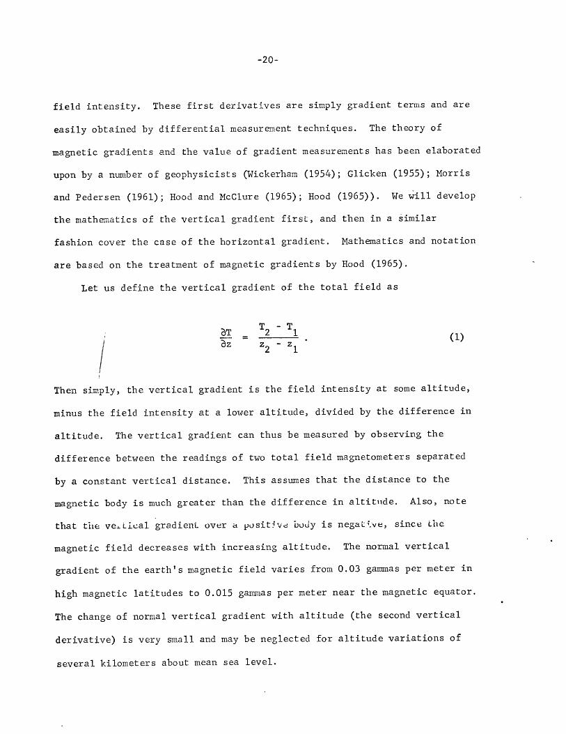
Let us define the vertical gradient of the total field as
T -TbT 2 1 (1)(1)
z z 2 - z I
Then simply, the vertical gradient is the field intensity at some altitude,
minus the field intensity at a lower altitude, divided by the difference in
altitude. The vertical gradient can thus be measured by observing the
difference between the readings of two total field magnetometers separated
by a constant vertical distance. This assumes that the distance to the
magnetic body is much greater than the difference in altitude. Also, note
that the vetLical gradient over a positive body is negative, since tile
magnetic field decreases with increasing altitude. The normal vertical
gradient of the earth's magnetic field varies from 0.03 gammas per meter in
high magnetic latitudes to 0.015 gammas per meter near the magnetic equator.
The change of normal vertical gradient with altitude (the second vertical
derivative) is very small and may be neglected for altitude variations of
several kilometers about mean sea level.
-21-
Gradients Over Geologic Contacts
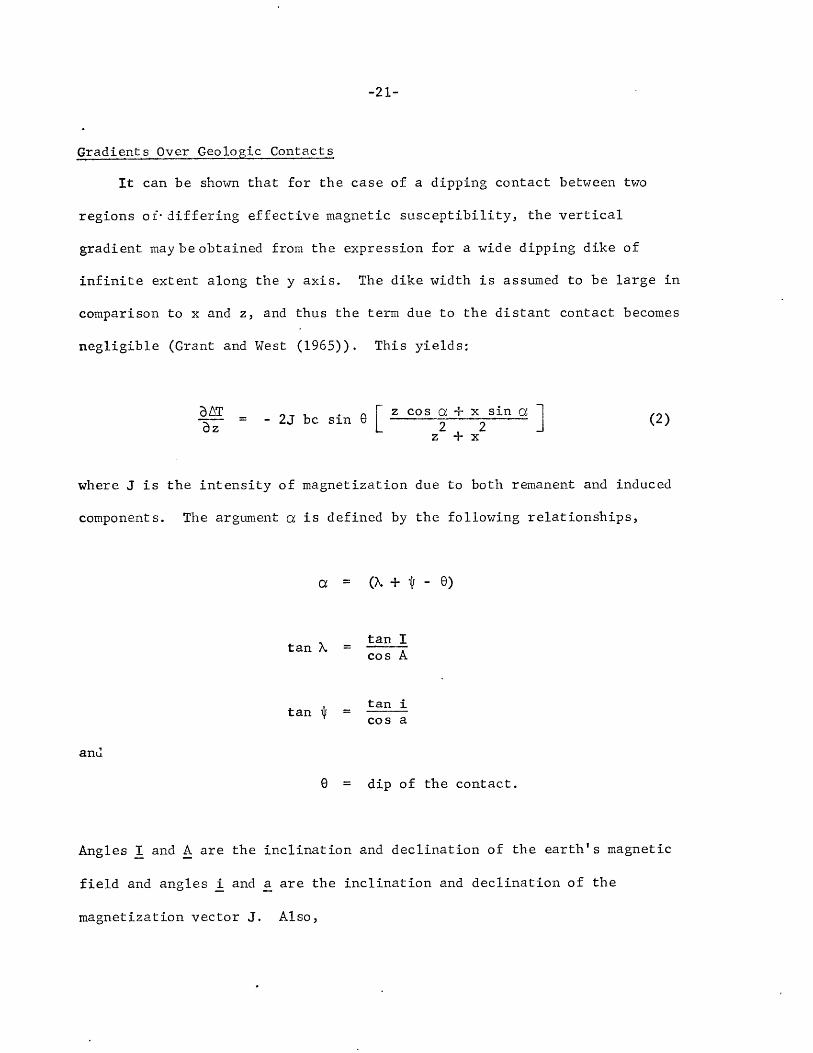
It can be shown that for the case of a dipping contact between two
regions of-differing effective magnetic susceptibility, the vertical
gradient maybeobtained from the expression for a wide dipping dike of
infinite extent along the y axis. The dike width is assumed to be large in
comparison to x and z, and thus the term due to the distant contact becomes
negligible (Grant and West (1965)). This yields:
BAT- - 2J
az
where J is the intensity of
components. The argument a
(2)bc sine [ z cos a + x sin a2 2
z + x
magnetization due to both remanent and induced
is defined by the following relationships,
a = (% + - e)
tan 2
tan 1
tan Icos A
tan icos a
and
G = dip of the contact.
Angles I and A are the inclination and declination of the earth's magnetic
field and angles i and a are the inclination and declination of the
magnetization vector J. Also,
-22-
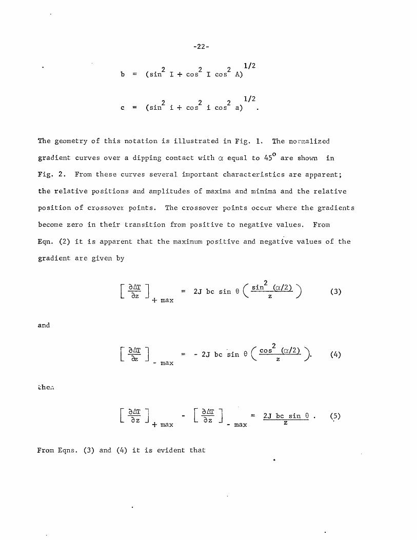
2 2 2 1/2b = (sin I + cos I cos A)
2 2 2 1/2c = (sin i + cos i cos a)
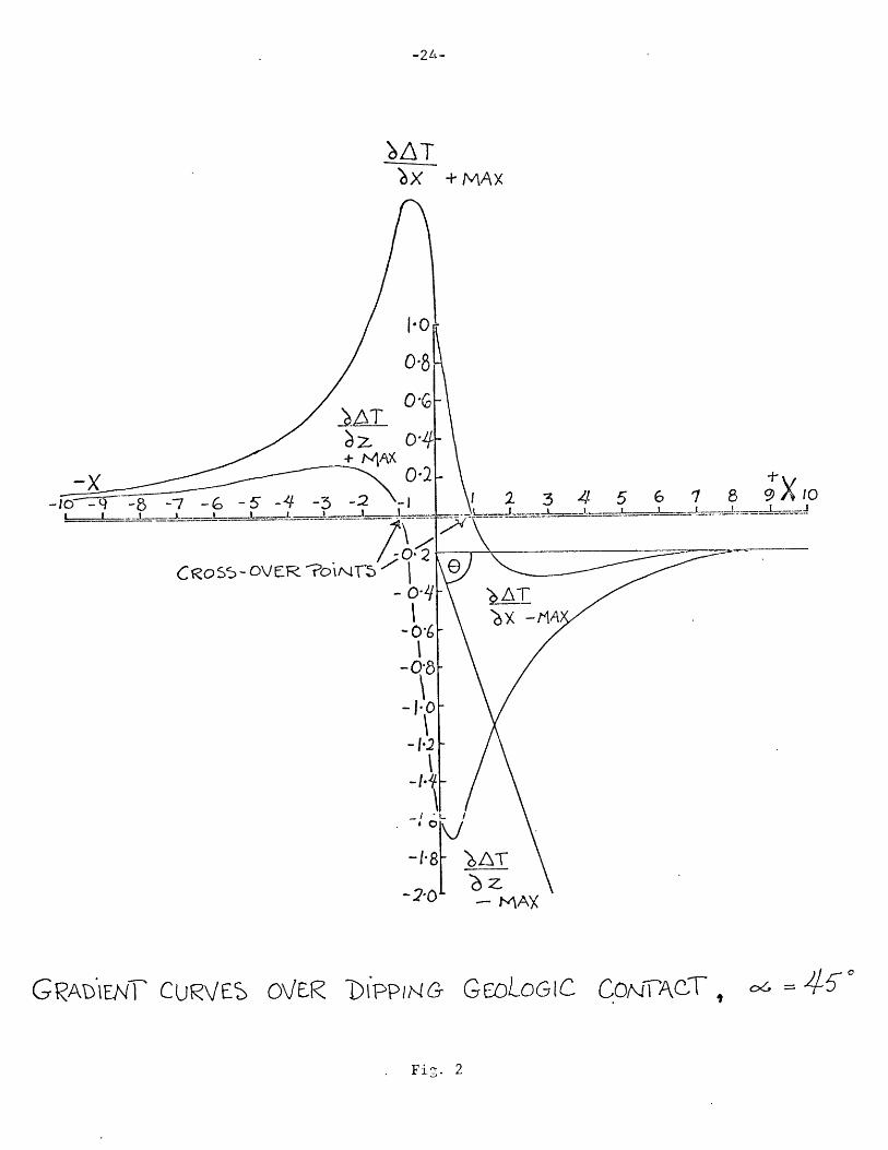
The geometry of this notation is illustrated in Fig. 1. The normalized
gradient curves over a dipping contact with a equal to 450 are shown in
Fig. 2. From these curves several important characteristics are apparent;
the relative positions and amplitudes of maxima and minima and the relative
position of crossover points. The crossover points occur where the gradients
become zero in their transition from positive to negative values. From
Eqn. (2) it is apparent that the maximum positive and negative values of the
gradient are given by
SAT m+ max
= 2J bc sin (sin 2 (a/2)
= - 2J bc sin 0 (cos 2 (/2)
- max
AT 1+ max
-z]- max
= 2J bc sin 0z
From Eqns. (3) and (4) it is evident that
and
(3)
[T
then
(4)
(5)

-2-
CLSOLOGIC CoNTAcTi-: MAGN4ET I C,
TCos I NORTH
J COS
-PLAN ViEIW
5 U 1FA C E
SEA FLORS* - *. * * * - . . . . * * * I
TCosI Cos A
Ih\
5ARTH '5MAGN ET'iC TiEL"D
/c
CR P055 'SECT 10NtAL
53EA
VE'-vDhPPI.NG- GEoOGICAL CONTAGF'
FCj. I
3 4 5 678 9X10
GRA .IE1- OVER k ) 1 puqc-.i GcoLoGLG CoNTiACT
Fis. 2
-24A-
-MT+ MAX
I
10-0-8
0,/=:6 5
c RO S5 - ov ER --?C),l N T-b

-25-
b[ AT1+ max
= - tan (a/2).- max
The horizontal distance between the maximum and minimum gradient is given by
x -x-max +max
cosec a= 2 z
The depth, z, to the top of the contact is then,
sin az = (X - x max)-max +max 2
(7)
or from Eqn. (6), letting
+ max= -t
- max
then
z = (X max- x max) L-max +tmax21+ t
(8)
The distance of the crossov C point f-), Lth origin ma3 be showi from
Eqn. (2) to be
- z cot a
(9)
= -2
X0 = Zf 2t
(6)
x0 =

-26-
Now let us consider the case of the horizontal gradient,
- 2J bc sin 0 2 2
z +x(10)
By combining Eqns. (2) and (10) the relationship between the vertical and
horizontal gradients can be shown to be
lAT x T + 2J bc sin 0 sin a+ (11)Ex z z z
Equivalent expressions for Eqns. (3) through (9) in the horizontal gradient
case are then:
+ max
[ %i ] - max
VAT + max
+ max
2J bc sin (co s (45 - (/2)) )
S- 2J bc sin 0 ( sin2 (450 - (a/2)) "z
[AT- max
. [ T
- max
T max+ max EaTI- max
= - cot 2 (450 - (rf/2))
= - t + 1 2t - 1
(12)
(13)
(14)
(15)

-27 -
cos CS= (-max- X+max 2
z = (x - max ) t)-max 2(1 + t 2 )
and the crossover point is given by
x0 = z tan a
or2t
o = - t2
(16)
(17)
(18)
Note that the upper edge of the contact always lies between the crossover
points of the vertical and horizontal gradient curves. The crossover
separation distance from Eqns. (9) and (18), can be shown to be
(x0)
bx
- (x0 )
8z
= z (tan a + cot a)
(19)x0 = z (l +t 2 )
2t(l - t2
We may obtain from the preceeding mathematical discussion a number of
interesting relationships between gradients and the parameters of geologic
contacts. These relationships enable us to make accurate estimates of
-28-
contact position, dip and depth.
It is apparent from Eqns. (9) and (18) that in high or low magnetic
latitudes, steeply dipping and nearly horizontal contacts are outlined by
the zero gradient contours. This is true so long as the direction of the
resultant magnetization, J, does not depart significantly from the geomagnetic
field direction; i.e., i = I and a = A. Specifically, steeply dipping contacts
in high magnetic latitudes (a = 900) and near the magnetic equation (a = -900)
are outlined by the zero vertical gradient contour. Nearly horizontal
contacts in high magnetic latitudes (a = 1800) and near the magnetic equator
(a = 00) are outlined by the zero horizontal gradient contour. For all
contacts at all latitudes the contact position lies between the zero contours
of the vertical and horizontal gradients.
Contact dip may be determined from the argument a if some knowledge of
the direction of the resultant magnetization, J, is available or assumed.
a is readily obtained from either the vertical or horizontal gradient by
Eqns. (6) or (15), or from the two combined by Eqn.(19). Essentially, though,
even with the aid of gradient information, contact dip and magnetization
direction remain inseparable. Neither one can be obtained from the data
i.ndependent of the ot'ler. However. for limiting cases -=ucI aC t1-: in high
and low magnetic latitudes the assumptions are simpler and independent
estimates, but not exact determinations, can be made.
Estimates of the depth to the top of a contact are unique and
independent of any assumptions regarding geomagnetic field or resultant
magnetization directions and intensities or contact orientation. Depth
-29-
estimates taken from gradients are therefore accurate and simple. They may
be made in a number of ways utilizing information from the horizontal and
vertical gradients singly or in combination. From any of the relationships
given by Eqns. (7), (8), (16), (17) or (19) we can estimate depth to buried
or hidden contacts.
/
-30-
Gradients Over Single Pole and Dipole Sources
Magnetic anomalies are often classified on the basis of their
resemblance to ideal anomalies originating from either a single pole or
dipole. These ideal magnetic anomalies can be simply described by
AT = C/rn
where
From Eqn.
AT is the amplitude of the anomaly;
C is a term which combines the effects of geometry and pole
strength;
r is the distance to the pole or dipole center; and
n is an exponent which governs the rate at which AT decreases
with increasing r.
(20) by differentiation with
2 2 2r =x + y +- z
we obtain a relationship which is known as Euler's equation:
AT AT ATx + yy + z z - nATax ay az (21)
n is 2 for a single pole,
n is 3 for a dipole.
(20)
where
and
-31-
Due to symmetry, at Tmax
zero arid thus we have
the first two terms, the horizontal gradients are
[bT ]max
nATmax
z(22)
From this relationship we may, be assuming z, determine the exponent n and
thus the source type. Or if we know the source type, we can assume a value
for n and determine the depth, z, to the source.
-32-
Gradients and Topography
Vacquier (1962) has shown that the magnitude and direction of
magnetization of a body can be computed from a knowledge of the shape of the
body and of the total field magnetic anomaly over the body. -The assumption
is made that the magnetization is uniform. The method is limited by the
accuracy of the magnetic survey, the extent to which the survey represents
only the anomaly due to the body in question, and the detail to which the
shape of the body is known. The method has been applied by Vacquier to a
number of isolated seamounts in the central and South Pacific with some
success. The calculation requires detailed and accurate topographic and
magnetic surveys of the area involved, as well as a large, high-speed
computer. The accuracy of the survey and the reduction of the data to
residual anomaly values appear to be the sources of greatest difficulty in
the actual application of this method.
Modification of Vacquier's method to accommodate gradient data, in
place of total field intensity data could improve the accuracy of the
calculation. In this case gradients offer several significant advantages.
1. The sensitivity of the gradients to anomalies arising from near
scurceq would emphasizc the ecfects of near topugrcDhv over those of deeper
geologic sources or more distant topography.
2. No corrections need be applied to gradient data in order to reduce
it to residual anomaly values.
These advantages should enable us to compute the direction and
magnitude of magnetization of isolated topography, such as seamounts, more
easily and with greater accuracy.
-33-
Computer Models
In order to investigate the relationship of gradients, total field
intensity, and field components to geologic structure a computer program was
written. The program computes anomaly profiles perpendicular to the axis of
two-dimensional, semi-infinite polygons of irregular cross-section.
Horizontal and vertical field component anomalies, the total field intensity
anomaly, and first and second vertical and horizontal derivatives are
computed and machine plotted by the program. Program documentation and
listings are included in Appendix 1.
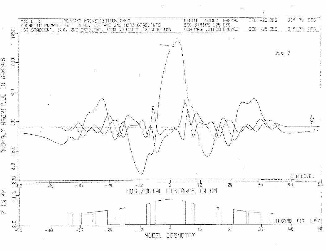
The following figures illustrate some of the more important
characteristics of magnetic gradients in relation to total field intensity
anomalies and specific geologic structures. Identifying information and
model parameters are given in a data block at the top of each figure. The
model cross-section is reproduced in the lower section of each figure.
Individual curves are identified by a single character, H, V, T, 1 or 2 at
their respective maxima.
Fig. 3 illustrates the greater resolution of gradients. The total field
anomaly and the first and second vertical gradients over three cubes 2 km on
e side, their top fccs at a depth of 4 km, are shown.
Fig. 4 illustrates the effects of topography on the total field
anomaly and the vertical gradients. The model is the same as in Fig. 3,
only one of the cubes now has a mansard roof. All other parameters have
remained unchanged.
Fig. 5 gives the horizontal gradients for the same model.

MUDE'- . . EMNRNT MAGNE1ZRAT TON ONLY FIELD 70000Mq1GNEIIC RNOVRLIES: TOTRL, 15T RN Z2ND VERTICRL GMROIENTS 5EC STR9IKE 90
'ST GRROIENT, 1rJX. 2NC CR OrENT . 100Y VE9TICRL XRGERRTTrON REM MRG .i0000
'f-RMMRSDEC.FMU/LC
DEC 0 DEG
DEC J
Fij
18.0 20o10
HORI70NIRL DISTRNCE IN KM
W BTIRD MT 1967
4.0-O
MODEL C.FOMETRY.0. 2.0 L.O0 i6.0 20.0
DIP u oE
GIP 80 DEG
. 3

MOiDEL. 4j REMNRNT* MPGW5?RTC1N UINLYII9GNETIC RINrLirL5, TO1TPLr I ST AND 2NUD VE9T ICRL GrLM0LT15T --qDj- 09 Vc -RLX
LnI
F IPL,0 70000SE.C 5091KE 909[M MRG .01000
GRMMRqd
EMU.' -CC
DEC 0 OEG 01 7 D0 r
O[C 0 DEG __ 80 P o3cDE
Fig. 4
cv -
ii 5SEA LEV[L5.0 6.0
HI ZCON TPL10.,0 12.0
DI5TPNCE I N KN
.0 2.0F~
W EBTRD KI!TVi'
MODEL GEOMETHY
2.0 1L I~.C 16.0 1r. 0
196F)7

MOD~EL. (4 9EMNRNT IARCRET~I RT I ON ONLYMRGNE-TfC: PRN0Mi.LIES, TFJTRL., 151 RND 2N-J riO'fRD~R%[T511 ro,13'" "'EI.NT, IlrJX'. 2ND Gf9PREWT r ICJ~lX VEf9Tl rI. L EX~c:rqTINI
FWLO70000 GPMMR$;SEC STJK 901 OEGflw MRSc .01 U00 EilJ/CC
DEC 0 DEG ol37 s OES~
0 Ec 0 DEG DIP 13U
Fig. 5
.13 2.0
.0 2.0
5ER LEVELI I I I . I - -
HH1ZUONTPL [U-1 J~ i t
N TiOF
16 0
1 ,iDEL L-EVMEl-,'Y
1~T 967~
C!) -
17',
cv -
............. i
- 4.0-
12 r]

-37-
Figs. 6 and 7 illustrate the combined effects of topography and
resolution for the vertical and horizontal gradients over a more complicated
model.
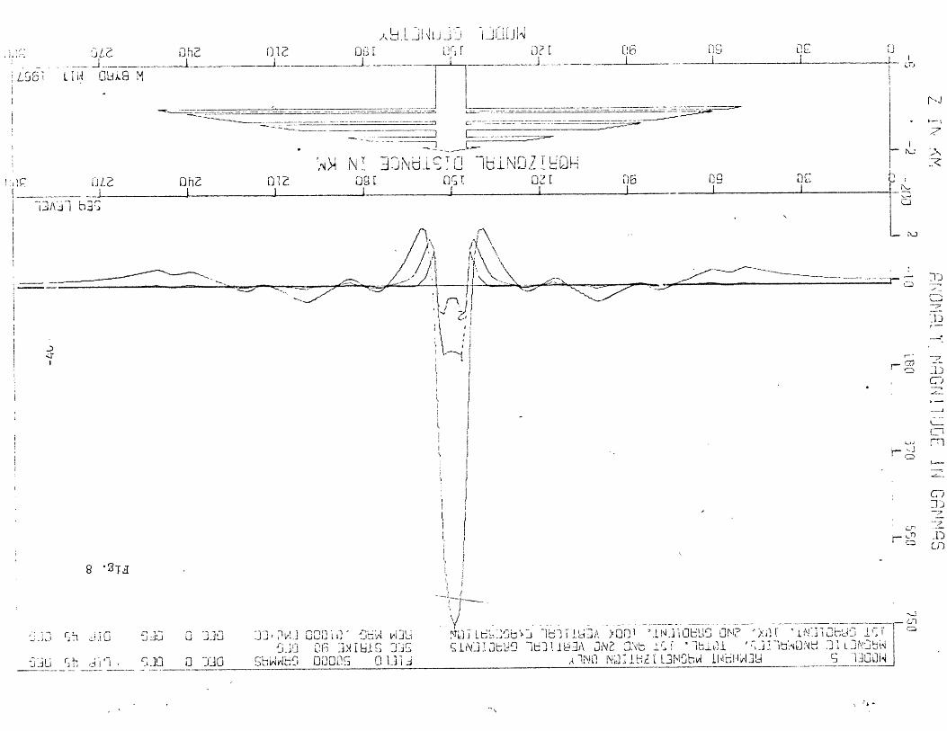
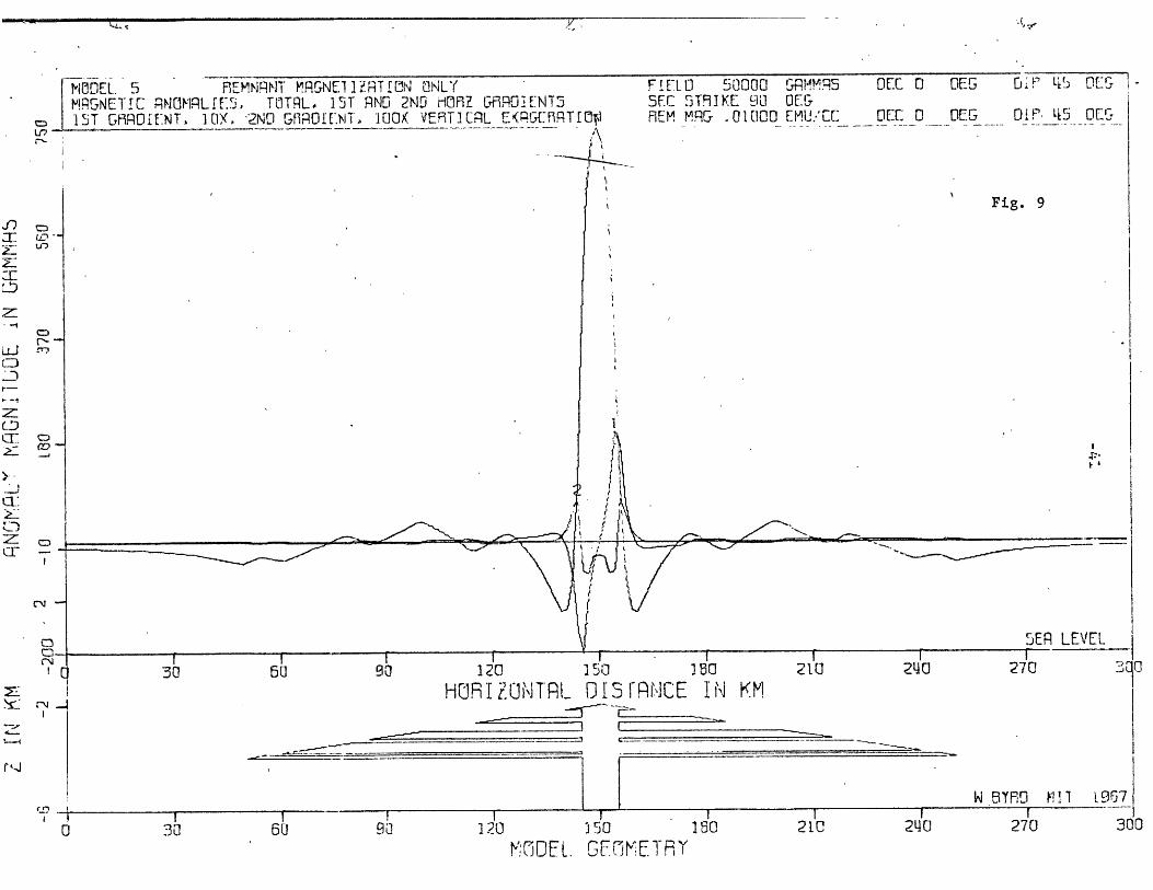
Figs. 8 and 9 illustrate the gradients and total anomaly over a "tree"
model. This model represents a volcanic ridge composed of horizontal lava
flows possessing alternately normal and reversed remanent magnetization.
The ridge strikes north-south and is located in mid-latitudes.
Fig. 10 illustrates the horizontal gradients and total anomaly over an
extremely complicated model. The value of a computer in performing such
calculations is apparent.
A more extensive display of the computer models generated in the course
of this work is available in Appendix 2./

M.LOE4," R3 ~ E M P'IT M qG9WD IF, TKR1LON UIN L'm r-i1 NE , L-rtl HC3Ht-19L FLh T iYFRL;, IF ') qI 2 N'li VE/PrpL ,FIPD1IENT5
15i ED I II[NT 1U/ 21L 59,R D.[N T V '1-- 9 T..'1L RL F X GRq9T 1 [ir
0 l 500005 EIL 3T73P1 125FIE t MP.-r -WI0 1O ,I- MIJ / cc
[WE l-25L
DIEC -25 DEG
/
DLT '75 IL-S
0 1, P 75 CF.E
Fig.
1~
/I
rn~
12111 2q1HOP[/OVITRIL U39EIHKM
.Eq LEVEL5- 4 F3
71 H
II H-12
Lr',i E R F
M r- D DL -DEOMKV1F--
91i 9r7I
*~- L')~ .1
CI
53K L-Th -2 L[
DER[ AMNqlMT M.qMLl "I ZHT r N DNi9LU IRYD FU5 T 0 T qL.~ 1 ' T\C 2N 1\f,-' L- R Z &9
Dmm~ h~ rUX rN.DlDN D ~T[LLORTUZr- -Q 0V,. I -RT O
FEJt 0 50CID 5rRMMRD fIEL -25 0115SECL 3[1-91 E 125 [IF5,9 p,- MR j .. 1 [ FM ',U'./ C DL 25O
Dr V? '7!
/ Fig. 7
U- 2
-3D HOP
HI5 It
5FR LFV[lE.
1. 12 2q -j '4T f:jil DI31PI11E N K%~M
W REHD MIT i9r
4 93-12
IMIU0 IL GF-lOMET1H9y
0
U-1I - 5
AdLj iLUa~~~a~ r1aaG l
N'> NTa h 7
ID N~Iu. 7biNOZI5[
I iI11AJ] b~
/ I
8 -2r
II i J I 1 0 a 1iGS~~k aaaw 0 l I AL'IiA
r~
z~-~ - __
'4/
T 0,~ Nil J I 1- IN S Nb 4 I I'iblL ~ __
I-.
,7z
IDEl
ciiElEl
I
MOD0EL 5 REMNRN-T ?IRrGNO f11'&;H J~l 01,,iLYMAGNETIC RNOFRLIE5, TO~TAL. 15IT RD 2NO H-09~Z C41ROME:NT5
S IJIT GHiROfINT. 10X, "2Nr0- GfIR01ffNTW *00 VE-I9TICRL CIOIR~0~
aD
F I ET1 50000 ! Plimps DEC 0 OEGY EV ~~[SEC 5T9IKE £10. UOIFiEtm MRrT -01(100 EMU:-J.*'r OmC 0 OE G D I P, LL5 J
Fig. 9
I
! I Iv SER LEVEL
120 250O ISOHUHPIYUNTPL UIM!1'.tNCE I N KM
2110 2140
21 r 2'40 270U
W BIRO W1 19637
120M;C'IUFL. GF(71MEITHy
IS 270Cl, I I 1 I
300
I I
4 _j
I

~1L~ I ' Y iM LUFJ r~TITL.~VTQ~ N 9fF. T~7Y~ 3LU. ITTE 1f I 72 1> rYiX \1~ I-NT fl-CJ T V '2LFL FXRGU-,FHP* ~IN1 E __ M ____ l f -
__ _ _ _ _ _ _ _ __ _ _ _ _ _ _ _ _ __ _ _ _ _ _ _ _ _ __ _ _ _ _ _ L IIt7 iLn
FIm -2 5 L-[I DIP 1 h F
D.C C l 1 J0' GE i EC FF
Fifg. 10
/A
)Er" LFVEL_13
F -D .:-
NVrp7-n 1 K F :
- V -
KU
E~D MITr
DU 70
Li
'I
L.J
1 ~KfF C- F
-20
-43-
A Marine Gradiometer System
The vertical gradient is, in general, more useful than the horizontal
gradient since it allows us to use the form of Euler's equation given in
Eqn. (22). Moreover, the horizontal gradient is derivable from the vertical
gradient by Eqn. (10). In certain cases, it may be more desirable to
measure the horizontal gradient or to measure both the vertical and horizontal
gradients together. The problems of designing a gradiometer system for either
the vertical or horizontal case are equivalent. We shall consider only the
vertical gradiometer. Vertical gradiometers for aeromagnetic work have been
described by a number of persons: Wickerham (1954), Hood (1965), Langan
(1966), Lynch et al (1966), Slack et al (1967). A surface-towed horizontal
gradiometer for marine use has been described by Breiner (1966). There
appears to have been no discussion of a vertical gradiometer for marine use.
We shall therefore examine the requirements for such a gradiometer in detail
and propose a possible system meeting these requirements.
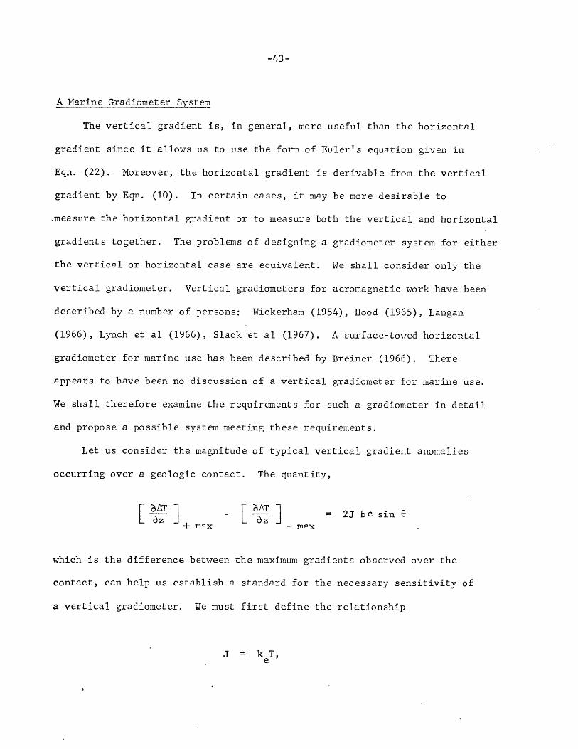
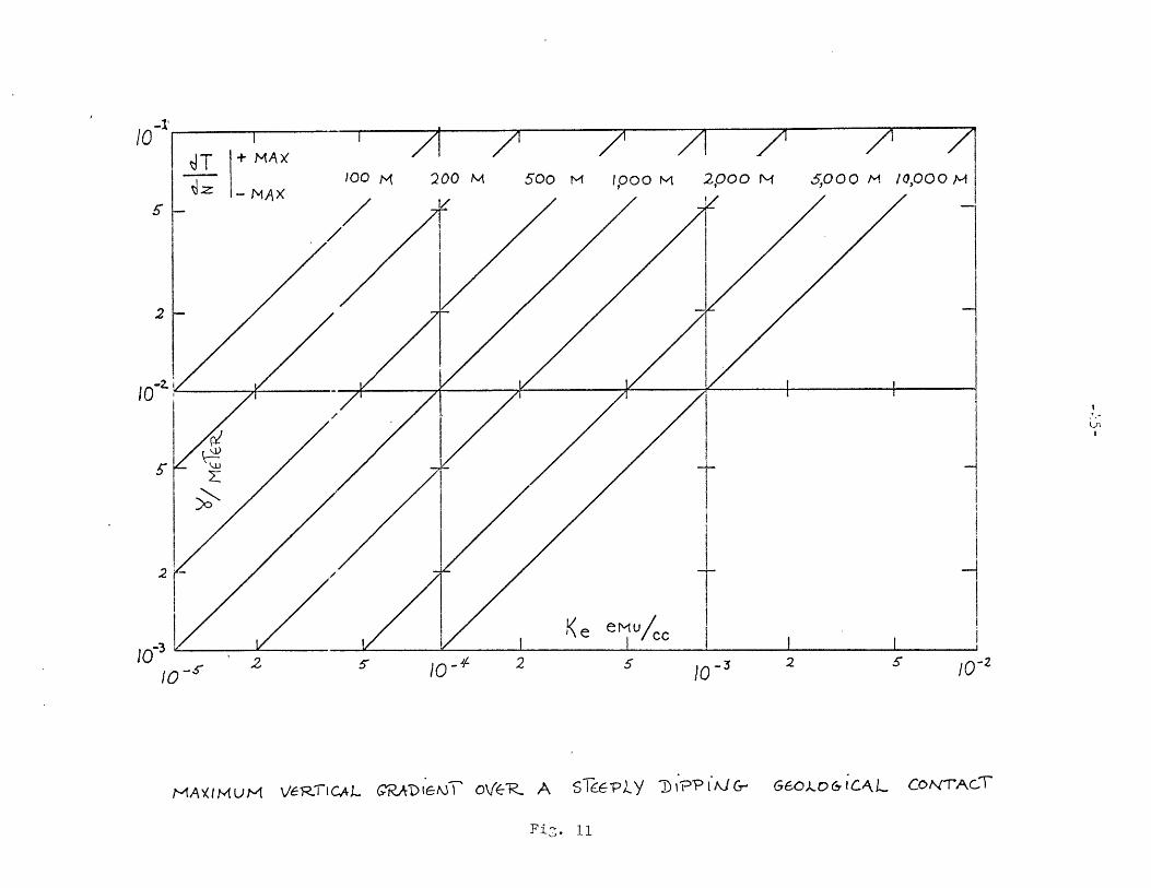
Let us consider the magnitude of typical vertical gradient anomalies
occurring over a geologic contact. The quantity,
S' T = 2 be csin 8
which is the difference between the maximum gradients observed over the
contact, can help us establish a standard for the necessary sensitivity of
a vertical gradiometer. We must first define the relationship
J = k T,e

-44-
where J is the intensity of the resultant magnetization, ke is the effective
susceptibility contrast across the contact, and T is the geomagnetic field
intensity. Fig. 11illustrates the variation of the maximum values of the
vertical gradient with effective susceptibility contrast, ke, and altitude,
z, above a steeply dipping contact in high magnetic latitudes where
bc sin e = 1.
If we take an altitude of 5 kilometers as representative of the ocean's
-3depth, and an effective susceptibility contrast of 10-3 emu/cc as
representative of oceanic basalt, then for this case the maximum vertical
gradient at sea level in the earth's field of 50,000 gammas would be 0.02
gammas per meter. This means that the anomalous gradient is the same order
of magnitude as the normal vertical gradient of the earth's field. A
useful gradiometer sensitivity might be 1% of the normal gradient, or
-42.0 X 10 gammas per meter. Since the rubidium vapor magnetometer has a
sensitivity of 0.01 gammas, an altitude difference, or sensor separation, of
100 meters would be required.
In order to maintain the errors due to variations in v(rtical
separation of the sensors near the level of the sensitivity, the vertical
spearation must remain constant within 151 or 1 meter. Since we have seen
that the horizontal anomaly gradient of the total field is the same order
of magnitude as the vertical anomaly gradient, Eqn. (14), position variation
away from true vertical must also be kept within I meter in order to keep
10
2
lo-z
S,
10- 310-
'DIIPl .AJ CON-rACT760),D&ICALt--lA)(IMUM V6IR:-IIC-AL CRADICNT' 0 V(-- IR - A
-46-
errors due to horizontal gradients at an acceptable level.
There are certain requirements to be met if we are to measure
successfully the vertical gradient at sea. First, a gradiometer must have
high sensitivity since the normal vertical gradient of the earth's magnetic
field is approxitately 0.02 gamma per meter. This requirement is met by the
gradiometer configuration of the rubidium vapor magnetometer. Second,
the gradiometer's two sensing elements must maintain a stable orientation
with respect to the earth's field. Their relative horizontal and vertical
separation must be predictable and constant within 17. The necessity for
a vertical separation of 10 to 100 meters between the two sensors precludes
any possibility of rigid mounting, especially since the gradiometer must be
towed at a sufficient distance to remove it from perturbations in the earth's
field arising from the ship's presence. Finally, sufficiently accurate
navigation must be available to assure close survey control and correlation
with other data such as topography, gravity, core samples, etc.
It is this author's contention that all of these requirements can be
met with existing, available, commerical equipment, and that the cost of
assembling and operating such a system as will be described would be
substantially less than .hat uf a deep-towed magnetometer capable of
procuring equivalent data.
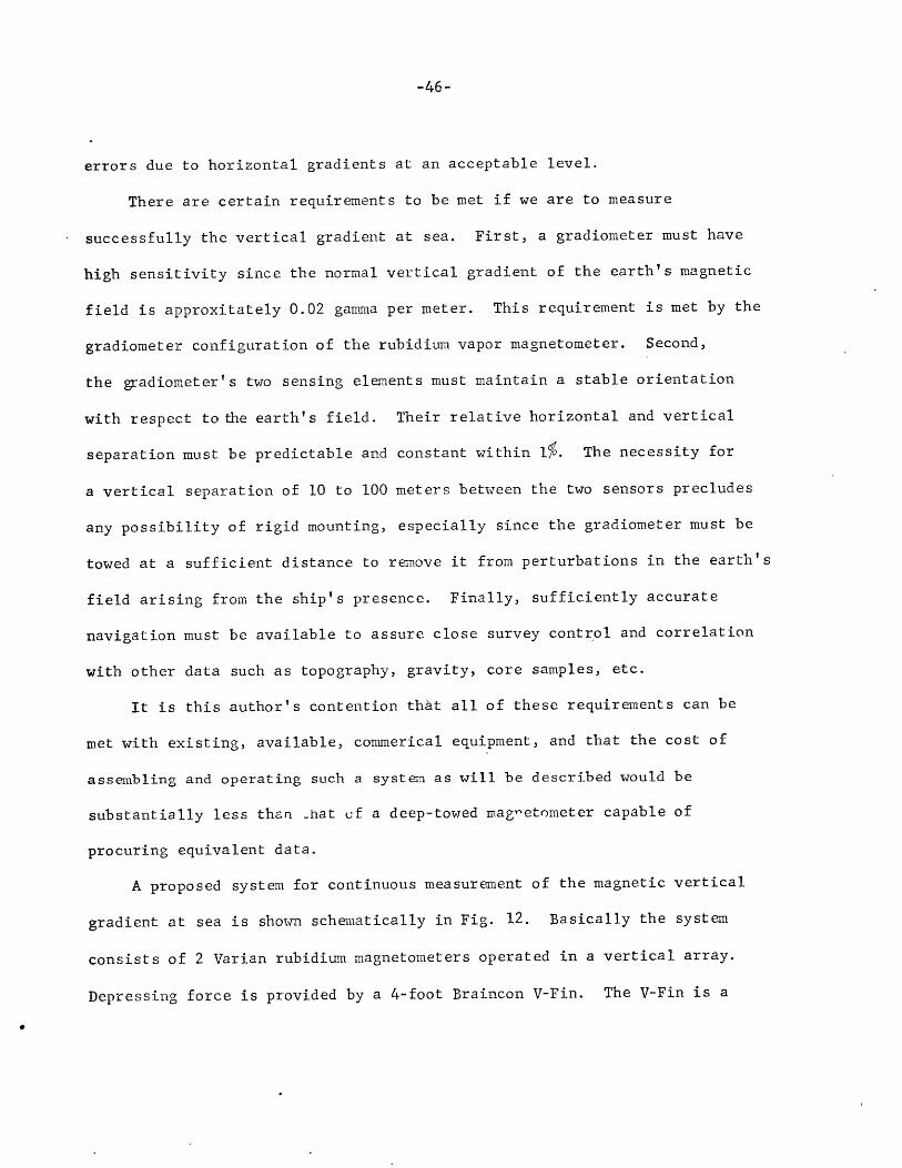
A proposed system for continuous measurement of the magnetic vertical
gradient at sea is shown schematically in Fig. 12. Basically the system
consists of 2 Varian rubidium magnetometers operated in a vertical array.
Depressing force is provided by a 4-foot Braincon V-Fin. The V-Fin is a
S U R EA
WELL LOGClN&
7ov\My? SPLYE. 5H P WIV17 E-\' 0UT UN IT
G 1; AP IC C01F-C E?;,..~ ........
L \Ft
-'R-6LL
ENO
100 -,,-20c mE-FE7-,
MAA ItWL-- CPkD OMTE SYSTEM
S E"F1 Ntq C ATO R
SFN5o 'LEs~CROI
10-1-001000 CBJ
METBR5
- L' V- F 7
Fig.
10 K'NOT5
I /I
12C14 E

-48-
hydrodynamically shaped underwater vehicle designed to maintain a stable
orientation and constant depth while being towed by a surface ship. Stability
is attained through a balance between hydrodynamic lift developed by the V-Fin
and drag on the tow cable. The V-Fin can be operated in either a positive
or negative lift configuration. The 4-foot V-Fin develops approximately
1,000 pounds of depressive force when towed at 10 knots, a reasonable ship
speed for survey type operations. The V-Fin provides stability and precise
depth control of the gradiometer baseline 100 to 200 meters beneath the sea
surface.
The V-Fin also carries the main instrument package containing the sensor
electronics,a depth transducer, water speed indicator, and a single
rubidium sensor. The second rubidium sensor is contained in a small
streamlined fish which is attached to the main tow cable by a short tether
at a point 10 to 100 meters above the main V-Fin. The length of the tether
is such that the two rubidium sensors are positioned vertically one above
the other. The necessary tether length remains nearly constant due to the
hydrodynamic characteristics of the V-Fin system, despite variations in
towing speed, so long as the distance between the two sensors is less than
one-half the towing depth, and towing speed is less theo' 10 to 12 knots.
Horizontal stability of the V-Fin is improved by addition of a vertical fin
near the tail. Horizontal and vertical stability of the upper fish is a
product of the short length of the tether (about 20 meters for a vertical
separation of 100 meters) and stabilizing fins on the fish itself. Launch
and retrieval of this system, at reduced ship speeds, should present no
great difficulty.

-49-
Electrical power is supplied at 28 volts D.C. from the ship, and signals
from the two magnetometer sensors and the depth transducer are returned to
the surface via conductors in the tow cable. The tow cable is armoured
one-half inch well logging cable with a minimum of six conductors including
two coaxial shielded pairs. The Larmor frequencies of the two sensors are
combined on board ship in the coupler and readout units to yield a beat
frequency proportional to the vertical magnetic gradient; this frequency
is approximately 4.667 cycles per gamma difference in total field intensity
between the two sensors. This signal along with the depth signal is recorded
graphically for immediate analysis and also on magnetic tape for later
computer analysis. Total field intensity may also be recorded from either
of the two sensors.
Effective use of magnetic vertical gradient information requires precise
navigation; knowledge of the ship's position to an accuracy of 0.1 kilometer
is necessary for high resolution surveys where ship tracks must be spaced
at intervals of several kilometers or less. Cruise plans for vertical
gradient measurements are therefore limited to ships possessing precise
navigation equipment, such as transit satellite navigation, or Loran C
within appropriate ar-as. Due to the excellent stability, lateral and
vertical, of the V-Fin system and the relatively short tow cable, the
position of the gradiometer array in relation to the ship is constant and
predictable. This simplifies the navigation problem considerably since only
the ship's position is required. It is anticipated that the capability for
precise navigation will soon be available as standard equipment on major
oceanographic ships engaged in geophysical research.

-50-
Gradient Error Sources
There are a number of sources of magnetic noise which we may expect to
produce errors in any attempt to measure magnetic field gradients at sea.
Let us investigate each of these sources, estimate the magnitude of the errors
involved, and see what can be done to reduce these errors. We will consider
the following error sources:
1. ship proximity;
2. atmospheric micropulsations;
3. water turbulence;
4. array position variations; and
5. instrument sensitivity and heading errors.
Ship proximity:
Errors in marine total field measurements produced by the distortion
of the earth's magnetic field in response to the presence of the ship
have resulted in the practice of towing the magnetometer sensor at a distance
of several ship lengths. For the measurement of gradients, the gradiometer
array should be towed at a greater distance from the ship, say 5 to 10 ship
lengths. Due to the sensitivity of gradients to near sources anomalies,
the increased tow length will reduce but not eliminate entirely the anomalous
effects of the ship. However, corrections could be applied by either of two
techniques. The magnetic field of the ship could be reduced or cancelled by
large demagnetizng coils similar to those used to protect ships from
magnetic mines. Or, the ship and the gradiometer array could be calibrated
in a magnetically quiet region in much the same way that a ship's compass is

-51-
calibrated. This would produce a correction curve as a function of the
ship's magnetic heading, enabling us to remove ship effects from the record
and establish a correct zero reference. Such a calibration would also be
effective in correcting instrument heading errors.
Atmospheric Micropulsations:
Because these effects originate in the upper atmosphere at relatively
great distance from the gradiometer array, their amplitude in the gradient
measurements are small. In addition, the sea water surrounding the sensors
acts to some extent as a shielding medium against time varying magnetic fields.
Because sea water is a relatively good conductor, electromagnetic disturbances
are attenuated in passage through it. Attenuation is by a factor of I/e at
a frequency, w, and a depth, d, which is the skin depth. The skin depth is
given by
d = -
where ji is the permeability of the medium; and
a is the conductivity of the medium.
For the case of sea w-ter.-7
p equals 4 X 10⁻⁷ mkgs units,
o equals 4 mho/meter,
and if
1ft 2 '

-52-
then the skin depth is given by
d 252 T 252//f meters.T
For a depth of 100 meters, then, attenuation to l/e or greater occurs for all
frequencies above around 6 cps. Attenuation at lower frequencies is negligible.
Water Turbulence:
It has been shown that the motion of ocean waves in the earth's
magnetic field gives rise to small alternating magnetic fields (Longuet-
Higgins et al (1954), Crews and Futterman (1962), Maclure et al (1964),
Warburton and Caminiti (1964), Weaver (1965)). These fields have the
frequency of the generating ocean waves and amplitudes, at the sea surface,
approaching 10 gamma for a long period swells of reasonable amplitude.
Warburton and Caminiti (1964) state that for the case of a 100 m wave with a
5 m height, 8 second period and sea state 6, the maximum field developed
varies from 3 gammas at the sea surface to approximately 0.1 gamma at a depth
of 100 meters. From Euler's equation (see Eqn. (22)) the vertical gradient
directly beneath the wave, assuming a dipole source (n equals 2) is then for
this case 2 X 10⁻³ gamjdciLser. This value is a factor of 10 less than the
average vertical gradient of the geomagnetic field. .rom this calculation,
it appears that if the gradiometer array is to be operated at sea state 6
the baseline of the array should be at least 100 meters or more below the
sea surface. The normal sea state at which magnetic survey work is likely
to be attempted will probably be less, perhaps 3 or 4, and under these

-53-
conditions a base line 100 meters below the surface should bring surface
wave generated gradients down to the sensitivity of the gradiometer.
Large-scale ocean currents such as the Gulf Stream also distort the local
geomagnetic field. However, their effect on the gradients are probably
small except in regions of extreme turbulence since these currents appear as
large-scale sources.
Array Position Variations:
Deviations of the sensors away from true vertical or variations
in their separation distance will produce errors in the gradient data which
are not easily corrected. For this reason every effort should be made to
insure that the towed array is as stable as possible. In order to keep
errors from this source below the sensitivity of the sensors, horizontal and
vertical position variations must be less than 17 of the separation distance,
or 1 meter for 100 meter separation.
Instrument Sensitivity and Heading Errors:
The sensitivity claimed by Varian Associates for their rubidium
vapor magnetometers is 0.01 gammas. In the gradiometer configuration the
sensitivity would be 0.02 gammas. The sensitivity varies with sensor
orientation and due to th, -Lbidium vapor magnetometer's design and
construction there are cerrain limitations upon the oensor's orientation
with respect to the total magnetic field vector. These limitations are
shown in Fig. 13. The optimum signal-to-noise ratio is obtained when the
sensor axis is inclined at 450 to the total field vector. The sensor will
not operate if its axis is either nearly parallel to or nearly perpendicular

i nop e e zones
Joki Fiel vec o
I oy IoIeienT,\Yjof IS
-30
I
Senso ORieCr,ATi on
Fig. 13
kLAc ti chKum
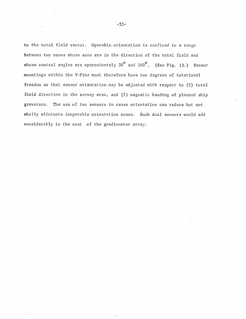
-55-
to the total field vector. Operable orientation is confined to a range
between two cones whose axes are in the direction of the total field and
whose central angles are approximately 300 and 1600. (See Fig. 13.) Sensor
mountings within the V-Fins must therefore have two degrees of totational
freedom so that sensor orientation may be adjusted with respect to (1) total
field direction in the survey area, and (2) magnetic heading of planned ship
graverses. The use of two sensors in cross orientation can reduce but not
wholly eliminate inoperable orientation zones. Such dual sensors would add
considerably to the cost of the gradiometer array.
-56-
References, Chapter I
Aitken, M. J., and Tite, M. S., "A Gradient Magnetometer using Proton Free
Precession," J. Sci. Instr. 39, 625--629 (1962).
Bloom, A. L., "Principles of Operation of the Rubidiurm Vapor Magnetometer,"
Applied Optics 1, 61-68 (1962).
Breiner, S., "Ocean Magnetic Measurements," Proc. IEEE Ocean Electronics
Synposiun (1966).
Crews, A., and Futterman, J., "Geomagnetic Micropulsations due to the Motion
of Ocean Waves," J. Geophy. Res. 67, 299--306 (1962).
Dean, W. C.,"Frequency Analysis for Gravity and Magnetic Interpretation,"
Geophysics 23, 97--127 (1958).
Glicken, M., "Uses and Limitations of the Airborne Magnetic Gradiometer,"
Mining Eng. 7, 1054--1056 (1955).
Grant, F. S., and West, G. F., Interpretation Theory in Applied Geophysics,
McGraw Hill, New York (1965)
Hall, D. H., "Direction of Polarization Determined from Magnetic Anomalies,"
J. Geophy. Res. 64, 1945--1959 (1959).
Hood, P., "Gradient Measurements in Aeromagnetic Surveying," Geophysics 30,
801--902 (1965).
Hood, P., and McClure, D. J., "Gradient Measurements in Ground Magnetic
Prospecting," Geophysics 30, 403--410 (1965).
Langan, L., "A Survey of High Resolution Geomagnetics," Geophy. Prospecting
14, 487--503 (1966).

-57-
Longuet-Higgins, M. S., Stern, M. E., and Stommel, H., "The Electrical Field
Induced by Ocean Currents and Waves, with Applications to the Method
of Towed Electrodes," Papers in Physical Oceanography and Meteorology,
MIT and WHOI 13, No. 1 (1954).
Lynch, V. M., Slack, H. A., Langan, L., "The Rubidium Vapor Gradiometer and
its Application in the Delaware Basin," Proc. Permian Basin Geophysical
Soc., 13th Annual Meeting (1966).
Maclure, K. C., Hafer, R. A., and Weaver, J. T., "Magnetic Variations
Produced in Ocean Swell," Nature 204, 1290--91 (1964).
Morris, R. M., and Pedersen, B. O.,"Design of a Second Harmonic Fluxgate
Magnetic Field Gradiometer," Rev. Sci. Instr. 32, 444--448 (1961).
Morrish, A. H., The Physical Principles of Magnetism, J. Wiley and Sons,
New York (1965).
Mudie, J. D., "A Digital Differential Proton Magnetometer," Archaeometry 5,
135--138 (1963).
Rikitake, T., and Tanaoka, I., "A Differential Proton Magnetometer," Tokyo
Univ. Earthquake Res. Inst. Bul. 38, 317--328 (1960).
Roman, I., and Sermon, R. C., "A Magnetic Gradiometer," Trans. AIME 110,
373--390 (1934).
Slack, H. A., Lynch, V. M., and Langan, L., "The Geomagnetic Gradiometer,"
Geophysics (in press).
Vacquier, V., "A Machine Method for Computing the Magnitude and the
Direction of a Uniformly Magnetized Body from its Shape and a Magnetic
Survey," Proc. of the Benedum Earth Magnetism Symposium (1962).
-58-
Warburton, F., and Caminiti, R., "The Induced Magnetic Field of Sea Waves,"
J. Geophy. Res. 69, 4311--4318 (1964).
Weaver, J. T., "Magnetic Variations Associated with Ocean Waves and Swell,"
J. Geophy. Res. 70, 1921--1929 (1965).
Wickerham, W E., "The Gulf Airborne Magnetic Gradiometer," Geophysics 19,
116-123 (1954).

-59-
II. A PROPOSED INVESTIGATION
OF MID-OCEAN EIDGE STRUCTURE
-60-
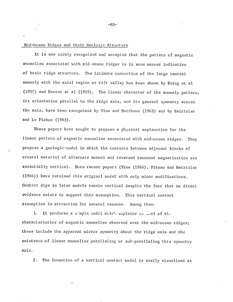
Mid-Ocean Ridges and their Geologic Structure
It is now widely recognized and accepted that the pattern of magnetic
anomalies associated with mid-ocean ridges is in some manner indicative
of basic ridge structure. The intimate connection of the large central
anomaly with the axial region or rift valley has been shown by Ewing et al
(1957) and Heezen et al (1959). The linear character of the anomaly pattern,
its orientation parallel to the ridge axis, and its general symmetry across
the axis, have been recognized by Vine and Matthews (1963) and by Heirtzler
and Le Pichon (1965).
These papers have sought to propose a physical explanation for the
linear pattern of magnetic anomalies associated with mid-ocean ridges. They
propose a geologic-model in which the contacts between adjacent blocks of
crustal material of alternate normal and reversed remanent magnetization are
essentially vertical. More recent papers (Vine (1966), Pitman and Heirtzler
(1966)) have retained this original model with only minor modifications.
Contact dips in later models remain vertical despite the fact that no direct
evidence exists to support this assumption. This vertical contact
assumption is attractive for several reasons. Among them:
i. It produces a s.mple .model whic: explains sc, al of th.-
characteristics of magnetic anomalies observed over the mid-ocean ridges;
these include the apparent mirror symmetry about the ridge axis and the
existence of linear anomalies paralleling or sub-paralleling this symmetry
axis.
2. The formation of a vertical contact model is easily visualized as
-61-
the result of a spreading sea floor process (Vine and Matthews (1963)).
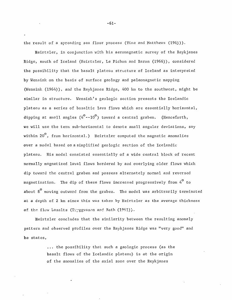
Heirtzler, in conjunction with his aeromagnetic survey of the Reykjanes
Ridge, south of Iceland (Heirtzler, Le Pichon and Baron (1966)), considered
the possibility that the basalt plateau structure of Iceland as interpreted
by Wensink on the basis of surface geology and paleomagnetic mapping
(Wensink (1964)), and the Reykjanes Ridge, 400 km to the southwest, might be
similar in structure. Wensink's geologic section presents the Icelandic
plateau as a series of basaltic lava flows which are essentially horizontal,
dipping at small angles (40--100) toward a central graben. (Henceforth,
we will use the term sub-horizontal to denote small angular deviations, say
within 200, from horizontal.) Heirtzler computed the magnetic anomalies
over a model based ona simplified geologic section of the Icelandic
plateau. His model consisted essentially of a wide central block of recent
normally magnetized laval flows bordered by and overlying older flows which
dip toward the central graben and possess alternately normal and reversed
magnetization. The dip of these flows increased progressively from 40 to
about 80 moving outward from the graben. The model was arbitrarily terminated
at a depth of 2 km since this was taken by Heirtzler as the average thickness
of the flow basalts (T:y1ggvason an Bath (1961)).
Heirtzler concludes that the similarity between the resulting anomaly
pattern and observed profiles over the Reykjanes Ridge was "very good" and
he states,
... the possibility that such a geologic process (as the
basalt flows of the Icelandic plateau) is at the origin
of the anomalies of the axial zone over the Reykjanes

-62-
Ridge cannot be denied on the basis of the analysis of
magnetic data.... The arguments for or against this
origin have to come from other geological or geophysical
considerations.
In summary, he states:
The geologic structure of Iceland is such that a
similar magnetic pattern, centered over the main graben,
is probably developed there. While such a geologic
structure could explain the axial magnetic pattern
observed over the ridge, the differences between the
Icelandic plateau and the Reykjanes Ridge are so large
that it is not clear to us how their geologic structures
can be similar.
This is the only serious consideration to date of the possibility that
the magnetic anomaly patterns observed over mid-ocean ridges may in fact
originate from a predominately horizontal layered structure rather than the
currently favored block structure of vertical dikes.

-63-
Vertical versus Horizontal Structure
The block structure model has several faults. The greatest of these
is that we do not find any evidence above the sea surface of vertical dikes
having the geographic extent and systematic orientation which the model
requires. This, despite the fact that portions of mid-ocean ridges stand
above sea level and thus are easily accessible. Without exception these
portions are volcanic islands, the largest of which is Iceland. The
structure of these islands is dominated by lava flows originating from
either point or line sources. There is no indication that any of the
mid-ocean ridge islands are the surface manifestations of a vertical dike
structure.
On the continents, vertical dikes are not uncommon, though they are
of limited extent and small scale. They account for only a small portion
of all volcanic activity. Large scale vulcanism invariably results in
extrusive activity and a horizontal or sub-horizontal structure. The
extensive plateau basalts of western North America illustrate this point
clearly.
The mid-ocean ridges exhibit many characteristics which indicate that
they are regions oft .ztrsive and activ- vulcanism. While the la-ge scale
topography of the ridges is gentle, due to their extensive lateral
dimensions, local topography, especially in the axial region, is extremely
rugged. Heat flow values along the ridge crests are typically 3 to 4 times
higher than the oceanic average (Von Herzen and Langseth (1966)).
Seismic activity is also high along the ridge crests, with epicenters being

-64-
closely associated with the topographic axis or rift valley (Ewing and
Heezen (1956)). Some mid-ocean ridges, notably those of the southwest
Pacific, are aseismic and exhibit normal heat flow along their crests. It
has been proposed that these are part of a now active ridge system which
has subsided (Menard (1964)). Dredge hauls and bottom photographs from
the mid-ocean ridges reveal that surface outcrops are volcanic in origin;
pillow lavas, vesciculated basalts and chilled, glassy surfaces are common.
It is difficult to conceive, in view of the extensive vulcanism which
is apparently characteristic of mid-ocean ridges, that the ridge structure
is not dominated by the same forces and constraints which operate in
terrestrial volcanic activity. The force of gravity, the viscosity of
molten rock, its thermal properties and its mode of cooling in a marine or
aeolian environment--all of these factors are similar on land or on the sea
floor.
Consider the following facts:
1. all mid-ocean ridges are, or have been in the past, sites of
extensive volcanic and seismic activity;
2. the outpouring of significant quantities of extrusive volcanics
is associated with such Activity;
3. the geologic structures produced by extrusive volcanic activity
are predominately horizontal or sub-horizontal in nature--not vertical;
4. extrusive volcanics are generally high in ferromagnesian mineral
content and upon cooling in the geo-magnetic field assume high remanent
magnetization.
-65-
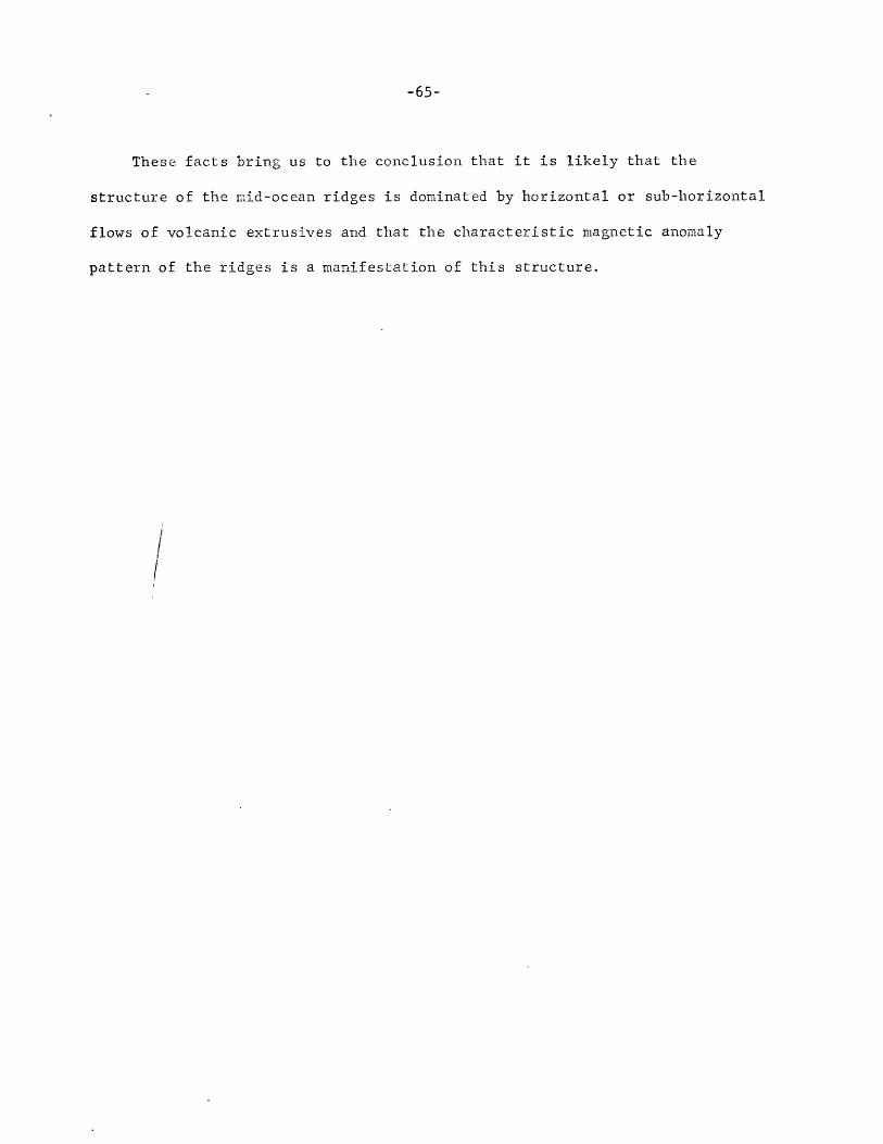
These facts bring us to the conclusion that it is likely that the
structure of the mid-ocean ridges is dominated by horizontal or sub-horizontal
flows of volcanic extrusives and that the characteristic magnetic anomaly
pattern of the ridges is a manifestation of this structure.

-66-
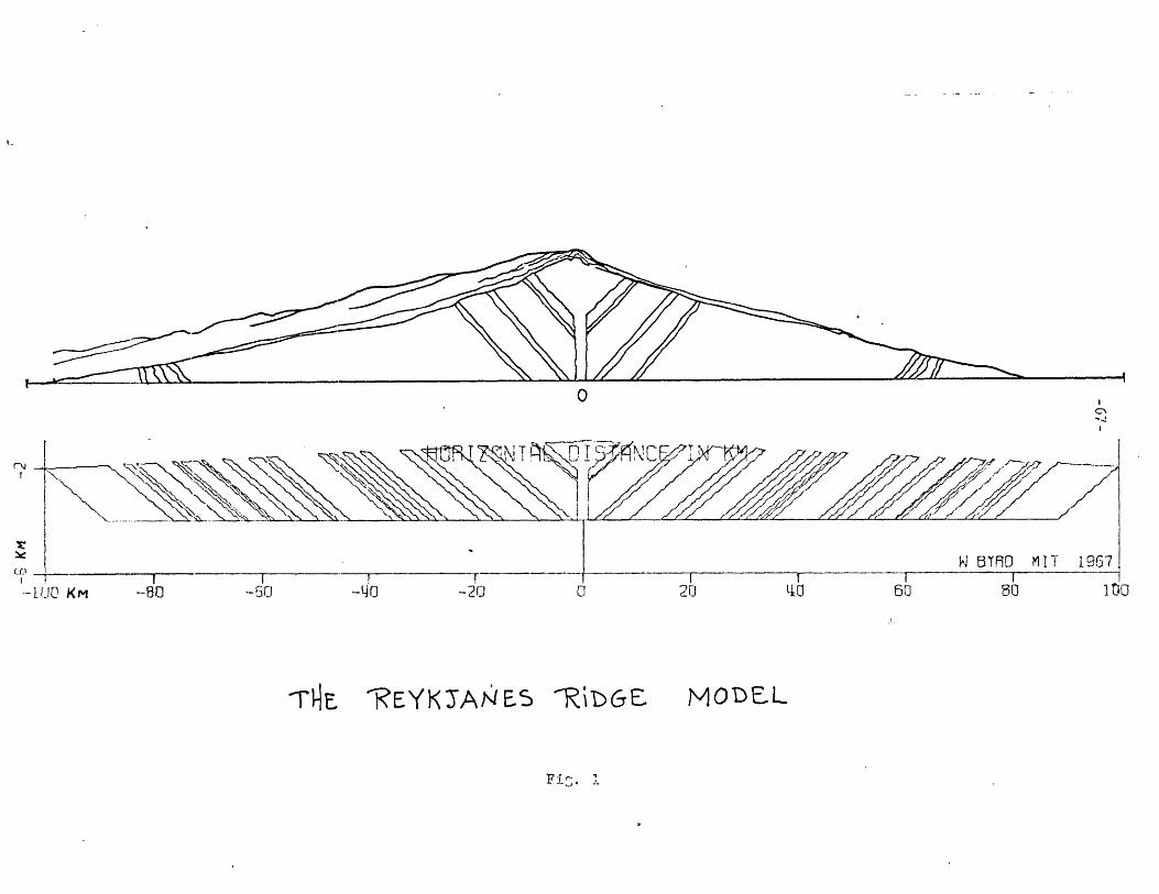
The Reykjanes Ridge Model
We developed the model in Fig. 1 in order to investigate the anomaly
pattern over a two-dimensional horizontal layered structure such as
Heirtzler assumed for his model of the Icelandic plateau. The purpose of
this investigation was to confirm the contention that.magnetic anomalies
similar to those observed over mid-ocean ridges could be produced by a
sub-horizontal layered structure. In addition, we sought to establish the
validity of a technique which would enable the determination of the
predominate orie-ntation of mid-ocean ridge structures.
Because the Reykjanes Ridge is one of the few regions which has been
the subject of a relatively extensive and accurate aeromagnetic survey
(Heirtzler et al (1966)), it was chosen as the region to which all model
parameters would be matched. The model of Fig. 1 is a two-dimensional,
sub-horizontal layered structure, with layers of alternate normal and
reversed magnetization of equal intensity. The model exhibits mirror
symmetry about its center axis, toward which each layer dips at 100. The
upper surface of the model is defined by smooth, sloping plane which is
intended to be representative of the average flank topography. The central
peak stnndqs km below sea lcve! 7n the flank slope is 1:109. The model
extends 100 km to either side of its center axis and thus the edges are
2 km below sea level. The bottom surface of the model is defined by a
horizontal plane 4 km below sea level. Thus the model has a thickness of
3 km along the center axis and 2 km along its edges. The horizontal
distance from the center axis at which the boundaries between layers of
0
W BTRfO MIT 196
LO -20 0 20 40 60r 0 1
"REYKIA NES -RDGE MODEL
Fin. i

-68-
normal and reversed magnetization outcrop of the topographic slope is
determined by the steepness of the topography, the dip of the layers, and
the thickness and number of layers present between a particular boundary and
the center axis. In order to generate the model of Fig. 1, values for all
of these parameters were assumed. The topography slope of 1:100 was chosen
as representative of flank topography along the Reykjanes Ridge. The layer
dip of 100 was taken as a typical value of the dip of basalt flows on the
Icelandic plateau (Einarsson (1960)). The number and thickness of the layers
was determined in the following manner. Distance of reversal points from
the center axis were taken from the geomagntic field reversal time scale
proposed by Pittman and Heirtzler (1966), using a conversion factor of
1 cm/year. These horizontal distances, in km, determine the outcrop position
of reversal boundaries on the topographic slope. The model possess a
central core of normally magnetized material 2 km in width and extending to
a depth of 3 km.
The remanent magnetization contrast was taken as 0.014 emu/cc,
corresponding to an alternately normal and reversed intensity of 0.007
which appears typical of oceanic basalts (Vogt and Ostenso (1966)).
Geonagnetic field paramiters ciara'eLcristic of the he:x' -anes Rid-g wcre
choosen (field intensity-- 50,000 gammas; declination--250 E; inclination--
750) and the model was positioned in the same orientation as the Ridge
(strike: NE-SW; 350 E true; 500E magnetic). Anomaly profiles were computed
on the MIT Computation Center's IBM 7094 and plotted under computer control
on an off-line Calcomp plotter. Calculation techniques are based on
-69-
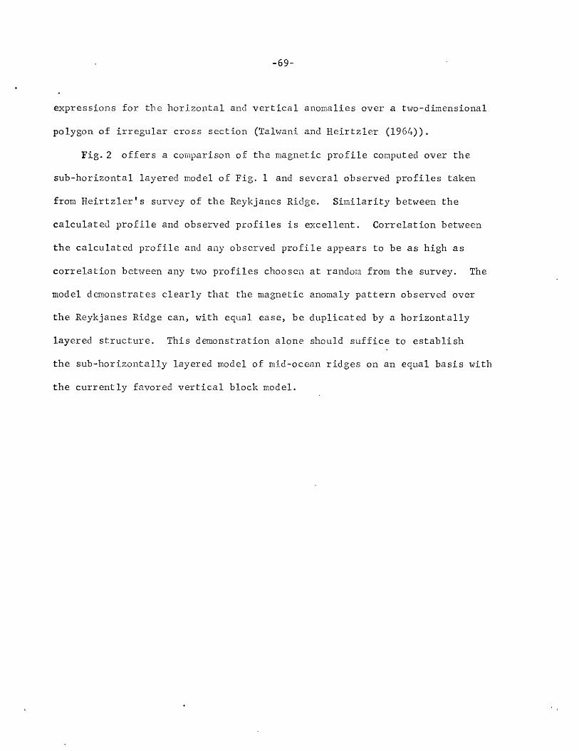
expressions for the horizontal and vertical anomalies over a two-dimensional
polygon of irregular cross section (Talwani and Heirtzler (1964)).
Fig. 2 offers a comparison of the magnetic profile computed over the
sub-horizontal layered model of Fig. 1 and several observed profiles taken
from Heirtzler's survey of the Reykjanes Ridge. Similarity between the
calculated profile and observed profiles is excellent. Correlation between
the calculated profile and any observed profile appears to be as high as
correlation between any two profiles choosen at random from the survey. The
model demonstrates clearly that the magnetic anomaly pattern observed over
the Reykjanes Ridge can, with equal ease, be duplicated by a horizontally
layered structure. This demonstration alone should suffice to establish
the sub-horizontally layered model of mid-ocean ridges on an equal basis with
the currently favored vertical block model.
MODEL 12 REMNRNT MRGNETIZRT I ON ONLYMRGWETIC RNiMRLIE5. TOTRL. HORZ NDO VE5TICRL COMPONENTS
FIELD 51600 C RMMqSSEC STRIKE 128 CElREN MRG 01400 EMU/CC
O:EC -25 DEC
ODE 0 DE
10S 010 0 0 E-o
-- 50
24
SER LEVEL
-60
This figure being photographed for scale adjustment.
Fig. 2
-71-
Logic of the Horizontal Structure
Both the vertical block model and the sub-horizontal layered model
are only conjectural and neither is supported by any direct geologic
evidence other than that offered by the basalt flow structure of the Ice-
landic plateau. The need for additional evidence enabling us to establish
the validity of either model is strikingly evident. In the absence of this
evidence let us examine the facts and assumptions which form a body of
indirect evidence making the sub-horizontal layered hypothesis of mid-ocean
ridge structure logically appealing.
1. The linearity and symmetry of the magnetic anomaly pattern observed
over mid-ocean ridges is easily produced by a sub-horizontal layered model.
2. The large central anomaly over the ridge axis can be produced by
a normally magnetized core similar to that contained in the model of Fig. 1.
3. The increasing wavelength of anomalies as one moves from the ridge
axis to the flanks can be produced in the sub-horizontal layered model by
decreasing topographic slope or layer dip in the flank region. Vine (1966)
and others have attempted to explain this change in character of the anomalies
by several fanciful schemes. One attributes the change to a sudden increase
in the frequency of geomagnetic field reversals about 25 million yenrs ago.
Another postulates variations in the rate of sea floor spreading with time.
Such explanations are unneeded if the structure of mid-ocean ridges is
horizontally layered.
4. The remanent magnetization intensity of the model of Fig; 1 is
uniform. There is no need to postulate that the intensity of the central
region is doubles in order to account for the relative magnitudes of the
-72-
central and flank anomalies (Vine (1966)).
5. According to reasoning which we have developed earlier, it is
likely that the structure of mid-ocean ridges is predominately horizontal
rather than vertical.
6. The sub-norizontal layered model of mid-ocean ridge structure is
entirely independent of, though not incompatible with, a spreading sea
floor hypothesis.
/

-73-
Methods for the Study of Ocean Ridge Structure
There are several lines of endeavor which we might pursue in an attempt
to gain more insight into the structure of mid-ocean ridges. The most
straightforward, and thus most impractical and impossible, of these would
be to conduct a conventional geological survey on the sea floor. We
cannot. Since the mid-ocean ridges are precisely what their name implies,
and lie beneath a kilometer or more of water, we are limited to dredge hauls,
bottom photographs, and perhaps a few visual observations from small
research submarines.
It would certainly be desirable to obtain oriented cores of the ridge
material in order to study the variation of remanent magnetization intensity
and direction in the vertical and horizontal dimensions. The JOIDES program
will attempt this. However, because of the expense and pressing need to
drill in otherlocations, the number of initial drilling sites located on a
mid-ocean ridge will be small, perhaps less than six. While this information
will be applicable to the problem of the ridge structure, it would require
extremely good fortune for this small amount of information to furnish us
an unambiguous answer.
Despite cores, photographs and heat flow measuremEnts, narinp
geophysics is primarily constrained to study the sea "floor from a distance
--from the sea surface. This observation from a distance is accomplished
by a number of techniques: seismic, gravimetric and magnetic--all of which
require the geophysicist to make assumptions and interpretations. It is on
the validity of his assumptions that the truth of his interpretation rests.
Joint Oceanographic Institutions Deep Earth Sampling (JOIDES (1965)).
_II_
-74-
In the question of the nature of mid-ocean ridge structure we are
dependent to a large extent upon information derived from a single technique,
magnetics. This is the case because in the ridge structure there is
evidently not any significant variation in density or composition associated
with the source of the magnetic anomalies. Thus seismic and gravimetric
studies tell us little about the structure which is evidently dominated
by the source of the magnetic anomalies. It is therefore necessary that
we utilize the information available from magnetics to the utmost extent of
our knowledge and ability.
Marine magnetic surveys are routine to the point of being automatic
and unimaginative. Typically they measure only the magnitude of the total
magnetic field intensity. Quite obviously the total magnetic field is the
sum of many fields and its intensity is the result of the influence of
many factors, some geologic, some not. In order effectively to utilize
magnetics in the study of geologic structure we must have some method
which enables us to separate geologic anomalies from regional trends and
temporal field variations (diurnals, micropulsations, secular changes, and
magnetic storms). One such method is the gradient aTi .ch (Hood (1965),
i!ood and McClure (196T)).
The gradient is effectively a filtering process. While the gradient
does not contain any more information than the original function (and in
fact, in a sense it contains less) the information is displayed or
re-arranged into another form which is more adaptable to analysis.

-75-
Magnetic Field Gradients
The gradient is the rate of change of some quantity with respect to
another quantity; it is a derivative. Thus there are potentially as many
gradients as there are variables. We shall concern ourselves with only two
gradients, the horizontal and the vertical, in the following discussion of
the application of geomagnetic field gradients to the problem of mid-ocean
ridge structure.
The horiz,ntal and vertical gradients of the total geomagnetic field
exhibit the fo l!owing useful characteristics:
1. Horizontal variations of these gradients emphasize the short
wavelength spatial components of magnetic anomalies, especially those
associated with contacts between regions of different effective magnetic
susceptibility.
2. Longer wavelength spatial components, such as those associated
with regional gradients and large scale structures, are highly attenuated.
3. Magnetic anomalies arising from near surface sources are greatly
enhanced over those arising from deeper or more distant sources.
4. These gradients contain an inherent zero reference which is
independent of the magnitude or direction of the total field, and of its
variations in time and space.
It is readily apparent from these characteristics that these gradients
are highly effective in delineating contacts or boundaries of near-surface
structures which are the source of total field magnetic anomalies.
Moreover, from the study of these gradients and their relationship to each
-76-
other, it is possible to draw certain conclusions regarding the nature of
the contacts involved.
Let us define the gradients in the following manner: the vertical
gradient,
BAT T2 - T1az Z2 - Z
and the horizontal gradient,
aAT T2 - T1
ax x 2 - x
where T is the total field intensity, the y axis is formed by the inter-
section of the contact and the horizontal x-y plane, x is perpendicular to
the y axis and z is vertical. The gradients are then simply the difference
in intensity of the total field at two points divided by the horizontal or
vertical distance between the points.
It can be shown that for the case of the dipping contact, the first
derivatives may be obtained from the expression for a wide dipping dike
where the thickness is large in comparison to x and z, and the term due to
the distant contact becomes negligible (Grant and West (1965)). This
yields,
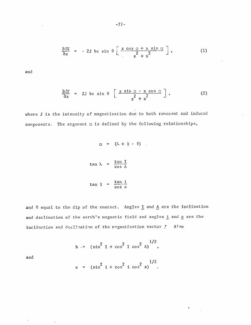
-77-
AT r z cos a + x sin a- L2J bsin O 2 2 1
z +x
T 2 bc sin 0 z sin a - x cos a-x 2 2
z +x
(1)
(2)
where J is the intensity of magnetization due to both remanent and induced
components. The argument a is defined by the following relationships,
C6= (% + * - 0)
tan
tan
tan Icos A
tan icos a
and 9 equal to the dip of the contact. Angles I and A are the inclination
and declination of the earth's magnetic field and angles i and a are the
inclination and dcclination of the magnetization vector j Also
2 2 2b .= (sin I + cos I cos A)
2 2 2c = (sin i + cos i cos a)
and
and
1/2
1/2
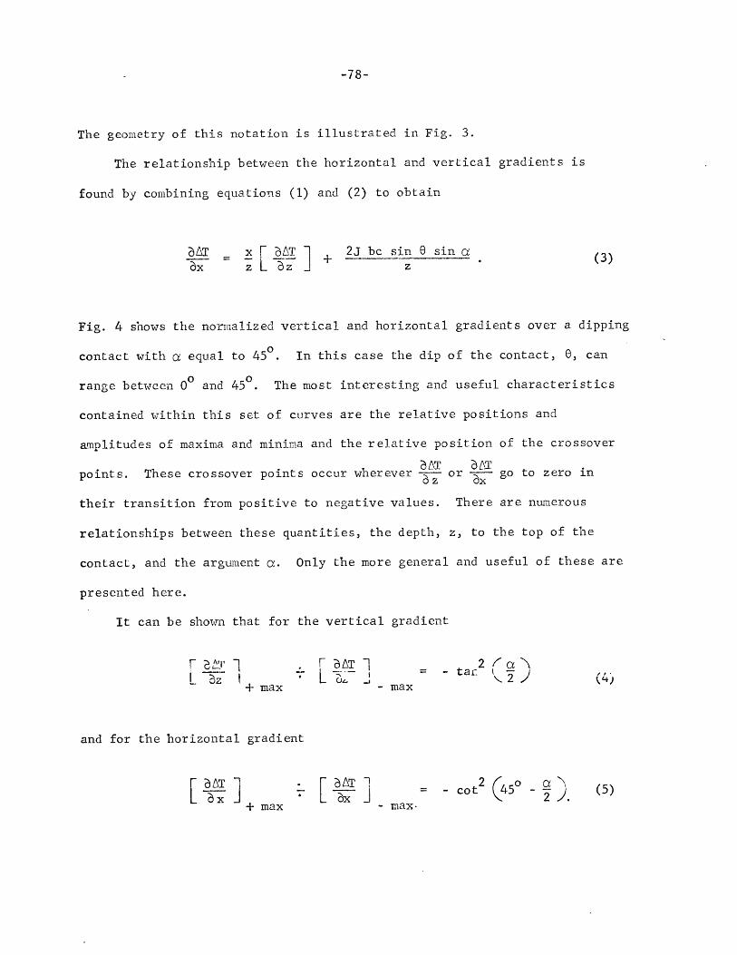
-78-
The geometry of this notation is illustrated in Fig. 3.
The relationship between the horizontal and vertical gradients is
found by combining equations (1) and (2) to obtain
BAT x [ T ] 2J bc sin 6 sin a(3)-+ (3)x z z z
Fig. 4 shows the normalized vertical and horizontal gradients over a dipping
contact with a equal to 450. In this case the dip of the contact, 0, can
range between 00 and 450. The most interesting and useful characteristics
contained within this set of curves are the relative positions and
amplitudes of maxima and minima and the relative position of the crossover
BAT BATpoints. These crossover points occur wherever Az or x go to zero in
their transition from positive to negative values. There are numerous
relationships between these quantities, the depth, z, to the top of the
contact, and the argument a. Only the more general and useful of these are
presented here.
It can be shown that for the vertical gradient
a T 2 (4L - = - t a f I , -
+ max -max
and for the horizontal gradient
T -~ 7bi J c2b 0 aATx ] = - cot 450 C' (5)+ max - max-
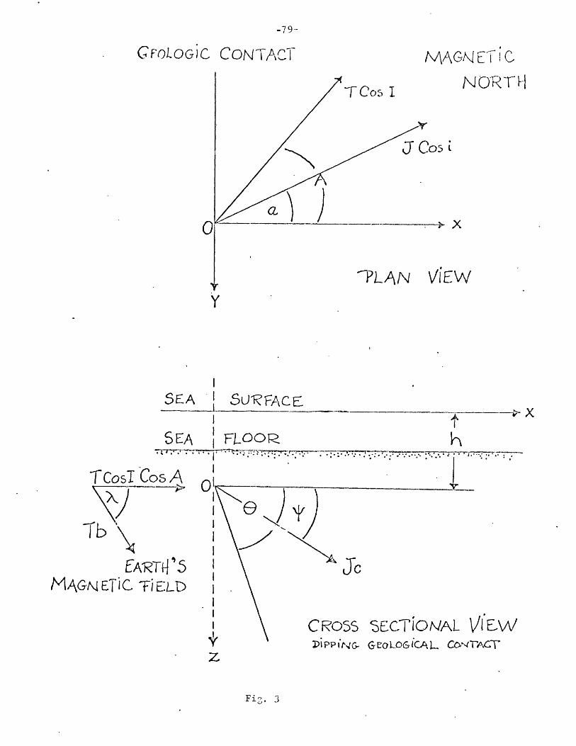
-79-
GFPOLOG JC CONT ACTi MAGN E-fC,
TCos I NOR TH
J Cos i
---- X
-PLAN VIEW
SU FACE
SEA FL00O
TCosT Cos A,
Tb
JcEA-RTO '5)MAGN ETiC T i ELD
C oSS SECTiONAL "V/E\A/GeoLOGiCA L C aNTACT
ISEA i
I
Z
Fig. 3

-0-
MATx + MAX
-7oRA-9 -F -7 -6
ShA~WtIV Cu)E OVER DIPutq&
2345618
GcoLoGiC CONCTI
Fig. 4
9A10
o6 r
oV C R*'?01 N -115

-81-
Also the distance between crossover points is given by
X0 = z (tan a + cot a). (6)
In addition, from Eqns. (1) and (2) it can be shown that
1_=
z +z Lx x+ max - max + max - max
2J bc sin 8= (7)z
Note that the contact will always lie between the crossover points of the
vertical and horizontal gradient curves.
From Eqns. (4) and (6) or (5) and (6) it is possible to obtain the
depth, z, to the top of the contact without any further assumptions
concerning the geometry of the contact or its relationship to the field and
magnetization vectors. Then by assuming values for the magnetization
intensity, J, and the inclination and declination of the field and
magnetization vectors, one can solve Eqn. (7) for the contact dip, 8.
Alternotively, any one of Eqns. (4), (5) or (C) cc-ld 1-e solved fcr the
argument a, and with the aid of a few simple assumptions, 0 obtained. The
necessary assumptions are not strict, especially if one is more interested
in knowing whether 0 is approximately 900 or 00 rather than knowing its
exact value. FigE. 5-6 illustrate the differences in the form of the gradients
over a section with vertical contacts and a section with sub-horizontal

-82--
contacts. For simplicity, the sections are assumed to be at high magnetic
latitudes where for the vertical case, a = 900, and for the horizontal
case a = 1800. FromFigs.5-- 6 it is easy to see that the major differences
between these two cases lie in the relationship of the gradients to the
zero reference line as described by Eqns. (4) and (5) and in the relationship
of the crossover points to each other, Eqn. (6), and to the position of the
top edge of the contact.
We must emphasize that the gradients do not add any new information
beyond what is already contained in total field data. We are still faced
with a number of ambiguities in any interpretation attempt based upon
potential field theory. In this case, the dip of the contact and the
direction of the resultant magnetization cannot be separated. We are unable
to solve for either of the two quantities independently. However, the
gradients are able (1) to eliminate the magnetic effect originating from
non-geologic sources; (2) to establish an accurate zero reference; and
(3) to provide a means enabling us to study the fine structure of magnetic
anomalies. For these reasons interpretations of geologic structure based
upon magnetic gradient data are likely to be more accurate and reliable.
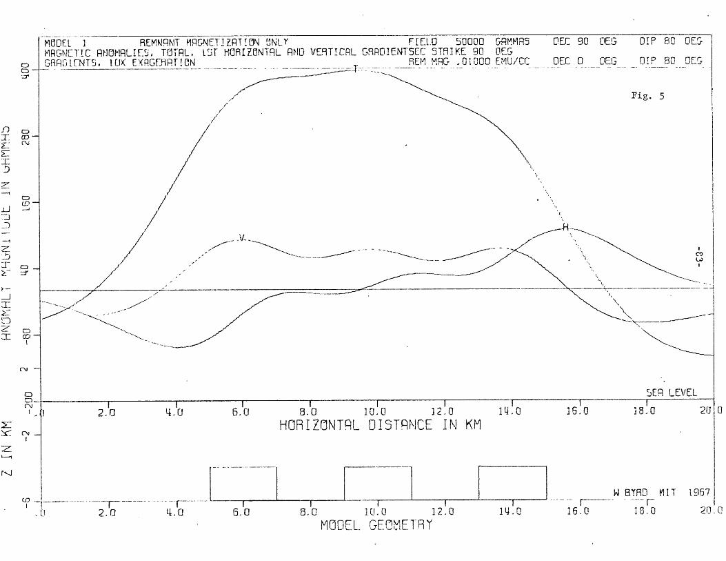
MtIIIL I REYKhRNT* MRGCNET1ZRTION £NL~y FAT EL.0 5s0000 CGRM*R5MRGMEITIC RHOM9LIES, T(ITRL. l'iF HOIfhZONTP.L RMID VEI9TCP.L G9,RGIENTSEC c-T91KE. 90 L1E1r
GEF~1A.__1.JXEXRGF.T!9 REM MRC? .01000 EMU/QC
GRR I NT, R!7
DEC 0 DEIGDIAP so D0.1-
0I .1. 00 E 15_
Fig. 5
I
//
/ 7
/
AL..
77~~'7
RI SER LEVELI.1 8010.0 12. -0
HORIZONITRL UI"3TRNCE IN KM
.02.0 4. 0 16.0I111.a0
MODEL_ G~E1]METH9Y
W BYR~D MI T
CD
-ZO
-No
2,0
N
4.0CIJ 161 18,0
1.9671
20,0,
c:)

This figure available June 6th.
-85-
Magnetic Gradients and Ocean Ridge Structure
In the case of a study of mid-ocean ridge structure there are a number
of approximations and assumptions which can be made to simplify the situation
even further. Vogt and Ostenso (1966) have shown that to a good approximation
the magnetization of oceanic basalts may be considered due entirely to
their remanent component. And to a first approximation, remanent
magnetizations established within recent geologic time--say the last ten
million years--can be considered parallel (normal or reversed) to the present
axial dipole field. A further simplification occurs in extremely high or
low magnetic latitudes where the effects of field inclination, expressed
by the sine and cosine terms, are either negligible or unity. Also, if we
chose as an area of study a region in which the ridge axis, and thus the
geologic contacts, run north-south, then the argument a simplifies to
a = (21 - 9) and bc = 1.0.
Depending on the specific region, any or all of these simplifications might
apply. Basically it is a rather simple matter to utilize the vertical and
horizontal gradients, either separatply or in conjunc:ion, to examine the
geologic structure of selected portions of a mid-ocean ridge. If exact
information concerning the intensity and direction of magnetization of the
ridge material is available--from, say, oriented cores--then one needs only
to make a gradient profile perpendicular to the ridge axis, regardless of
magnetic latitude or orientation of the ridge structure relative to the

-86-
geomagnetic field. Lacking core information, it is possible to choose a
region in which the geometry of the earth's field and the ridge structure
combine to reduce both the complexity of the problem and the number of
necessary assumptions.
Theoretically, of course, it is possible to abstract the same
information from a total field profile as from a gradient profile. In
practice, however, the overlap of time and spatial domains to which the
total field profile is subject results in a low signal-to-noise ratio. Also,
the total field profile must be reduced to a residual anomaly proifle in
order to remove large scale regional effects. The accuracy of this
reduction is not sufficient for the determination of a useful zero
reference level, or for the mathematical determination, from the total field
profile, of the gradients to sufficient precision to permit their extensive
interpretational use. The direct measurement of gradients, by establishing
an accurate zero reference and by eliminating the need for residual reduction
and diurnal corrections, presents a high resolution method for the study
of small scale magnetic anomalies of geologic origin. The sharp definition
of such anomalies on gradient profiles permits an accurate determination of
depth to the source bcay as well as the position qnd nature of the source
boundaries.
-87-
Conclusion
We have demonstrated clearly that the pattern of magnetic anomalies
observed over mid-ocean ridges can originate from a sub-horizontally
layered structure composed of lava flows having alternately normal and
reversed remanent magnetization. We have attempted to outline the logic
which favors such a structure over the vertical block structure proposed
by the currently favored hypothesis of sea floor spreading.
The superiority of the sub-horizontal structure hypothesis does not
necessarily imply that the concept of sea floor spreading is invalid.
However, the mechanisms and processes involved in sea floor spreading and
their relationship to the structure of mid-ocean ridges must differ to a
marked extent depending on the actual character of the ridge structure.
We should undertake, for this reason, further and extensive efforts to
delineate the geologic structure of mid-ocean ridges. The relationship
of this structure to observed magnetic anomaly patterns and to the
hypothesis of sea floor spreading occupies a central position in our
attempts to understand the global processes which have produced the pattern
of continental and oceanic regions which we know today.
Just as magnetic anomaly profiles have produced much information
and conjecture concerning the nature of the mid-ocean ridges, so directly
measured gradient profiles hold great promise as a method for further
study of the ridge structure. From horizontal and vertical gradient
measurements local scale magnetic anomalies can be more easily and
accurately recognized, defined and analyzed. Depth to source, source

-88-
character, and boundary contact position and orientation can be made from
gradient measurements with fewer assumptions necessary on the part of the
interpreter. The gradient method offers an attractive solution to the
problan of determining the predominate orientation of the ridge structure.
We propose to resolve this problem by determining the contact dip between
regions of differing magnetization along the ridge axis. This determination
can be made with the aid of direct measurements of horizontal and vertical
gradients of the total magnetic field.
If the hypothesis that the ridge structure is predominately
sub-horizontal in chracter is confirmed, then a re-examination of the
spreading sea floor hypothesis in the light of this new evidence is required.
It is unlikely that the spreading sea floor hypothesis would survive such a
re-examination in so elegantly simple a form as it now exists.
-89-
References, Chapter II
Einarsson, T., "The Plateau Basalt Areas in Iceland," On the Geolaogy_ and
Geophysics of Iceland," Int. Geological Congress, XII Secction (1960).
Ewing, M., Heezen, B. C., and Hirshman, J., "Mid-Atlantic Seismic Belts and
Magnetic Anomalies," (abstract), Common. 110-bis Assoc. Seismol.
Assemblee Gen. UGGI, Toronto, Ontario (1957).
Ewing, M., and Heezen, B. C., "Some Problems of Antarctic Submarine Geology,"
Geophysics Monograph 1, 75--81, Am. Geophy. Union, Washington, D. C.
(1956).
Grant, F. S., and West, G. F., Interpretation Theory in Applied Geophysics,
McGraw Hill, New York (1965).
Heezen, B. C., Tharp, M., and Ewing, M., "The Floors of the Oceans, 1, The
North Atlantic," Geol. Soc. Am., Special Paper 65 (1959).
Heirtzler, J. R., Le Pichon, X., and Baron, J. G., "Magnetic Anomalies over
the Reykjanes Ridge," Deep Sea Res. 13, 427--443 (1966).
Heirtzler, J. R., and Le Pichon, X., "Crustal Structure of the Mid-Ocean
Ridges, 3. Magnetic Anomalies over the Mid-Atlantic Ridge," J. Geophy.
Res. 70, 4013--4033 (1965).
JOIDES (Joint Oceancgr phic Institutions' Deep Earth Samnli.g Progrp= ),
"Ocean Drilling on the Continental Margin," Science 150, 709 (1965).
Menard, H. W., Marine Geology of the Pacific, McGraw Hill, New York (1964).
Pittman, W. C., and Heirtzler, J. R., "Magnetic Anomalies over the Pacific-
Antarctic Ridge," Science 154, 1164--1171 (1966).
-90-
Talwani, M., and Heirtzler, J. R., "Computation of Magnetic Anomalies
Caused by Two-Dimensional Structures of Arbitrary Shape," Computers
in the Mineral Industries, Stanford University Press, Geol. Sci.
Vol. IX, No. 1 (1964).
Tryggvason, E., and Bath, M., "Upper Crustal Structure of Iceland," J. Geophy.
Res. 66, 19 (1961).
Vine, F. J., "Spreading of the Ocean Floor: New Evidence," Science 154,
1405--1415 (1966).
Vine, F. J., and Matthews, D., "Magnetic Anomalies over Ocean Ridges,"
Nature 199, 947--949 (1963).
Vogt, P. R., and Ostenso, N. A., "Magnetic Survey over the Mid-Atlantic
Ridge between 420 N and 460 N," J. Geophy. Res. 71, 4389 (1966).
Von Herzen, R. P., and Langseth, M. G., "Present Status of Oceanic Heat
Flow Measurements," Physics and Chemistry of the Earth, Pergamon Press,
Oxford (1966).
Wensink, H., "Paleomagnetic Stratigraphy of Basalts and Intercalated
Plio-Pleistocene Tillites in Iceland," Geol. Rundsch. 54, 364--384
(1964).

-91-
Appendix 1
A PROGRAM FOR COMPUTATION AND PLOTTING
OF MAGNETIC ANOMALIES AND GRADIENTS
OVER 'TIO-DIMENSIONAL POLYGONS OF IRREGULAR CROSS-SECTIONS
/
-92-
This program has been w ritten in Fortran II for use on the IBM 7094 of
the MIT Computation Center. The system requires slightly less than 20,000
words in memory with all subroutines included. The program consists of a
main program which performs all calculations and produces printed output,
and a block of subroutines under the single call name of PLOTS whose function
is to produce a graphical representation of the printer output on an off-line
Cal-Comp plotter. Two versions of the program exist; one with a dummy PLOTS
subroutine for users who do not wish to use any of the plotter options (this
version requires only 10,000 words in memory and will compile and setup
much quicker); and the complete version which contains numerous plotter
options which enable the user to specify the form and content of the plotter
output.
The main program has been modified and expanded from a program published
by Talwani and Heirtzler (1964). The program computes the anomaly profiles
for total field, horizontal and vertical components, first and second
vertical derivatives and first and second horizontal derivatives over a
uniformly magnetized two-dimensional polygon of irregular cross-section.
Polygons of up to 199 3iCs are permitted. The profiles generated are at
right angles to the polygon axis. Gradients are obtained from differences
in total field intensity at two or more points separated horizontally or
vertically by a distance specified by the user. Anomalies are computed at
a number of discrete points along the profile. Number and separation of
these points is under user control. The total number of computation points
may not be greater than 200. Printed output provides the anomalies in two

-93-
forms. The first utilizes the standard approximation
AT = AH cos A cos I + AV sin I (1)
where AT is the total anomaly intensity,
AV is the vertical anomaly intensity,
LH is the horizontal anomaly intensity,
A is the declination of the earth's magnetic field referred to
the x or traverse axis (see Fig. , section ), and
I is the inclination of the earth's magnetic field.
The second form of the anomaly output, which is not an approximation,
is the magnitude of the vector sum of the horizontal anomaly, the vertical
anomaly and the earth's magnetic field, minus the intensity of the earth's
field. Mathematically this is
AT = + AV+T - T (2)
All plotter output utilizes this more correct form of the anomaly.
The PLOTS subroutin produces graphical representations of the model
structures and anomalies computed by the main program. All plots are drawn
to standard 8-1/2 by 11 inch size, spaced automatically along standard
Cal-Comp plotter paper. The user may specify certain plotter options which
enable him to obtain plots of selected anomaly profiles only. Scales are
chosen by the computer on the basis of the range of data to be plotted; this
-94--
ensures optimum use of the space allocated for the plot. However this
practice will result in non-uniform scaling in normal use. If the user
requires uniform scaling, it is suggested that he rewrite the appropriate
statements in the PLOTS subroutine.
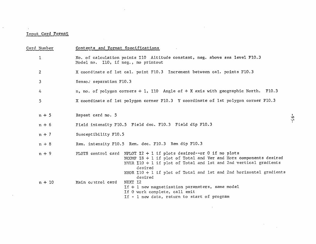
Input Card Format
Card Number
1
2
3
4
5
n+6
n + 10n + 10
Contents and Format Specifications
No. of calculation points I110 Altitude constant, neg. above sea level F10.3Model no. Ii0, if neg., no printout
X coordinate of 1st cal. point F10.3 Increment between cal. points F10.3
Senso: separation F10.3
n, no. of polygon corners + 1, 110 Angle of + X axis with geographic North. F10.3
X coordinate of 1st polygon corner F10.3 Y coordinate of 1st polygon corner F10.3
Repeat card no. 5
Field intensity F10.5 Field dec. F10.3 Field dip F10.3
Susceptibility F10.5
Rem. intensity F10.5 Rem. dec. F10.3 Rem dip F10.3
PLOTS control card NPLOT 12 + 1 if plots desired--or 0 if no plotsNCOMP 18 + 1 if plot of Total and Ver and Horz components desiredNVER 110 + 1 if plot of Total and Ist and 2nd vertical gradients
desiredNHOR 110 + I if plot of Total and 1st and 2nd horizontal gradients
desiredMain ccatrol card NEXT 12
If + 1 new magnetization parameters, same modelIf 0 work complete, call exitIf - 1 new data, return to start of program

-96--
FORTRAN II IB1I 7094 2D MAGETICS FIELD CO,..,u;.NENTS AND GRADIENTS
11 BYRD 1.ii DEPT OF GEOLOGY AND G-OPHySTC 1967MODIFIED FF.ROii 1ALWANI AND HEI RTZLFR F'kuGRA',i
WITH PLOT OPTIONDIMENSION ZEE(200),H(5),V(5),T(5),TP(5),FX{59200),PSU'i(59200),OSU
1(5,200)DIMENSION TOTAL(200),VGRD(200),VGRD2(200),HGRD1(200)oFI-GRD2(
2 00)9H1C(200),VC(200)oZ(200) X(200),EXX(200)
COM>,0ON TCTAL,VGRD1,VGRD2 9 HGRD1,HGRD2 ,HCVC ZX9EXX eJTOT,KTOT 9 IDENT
1,FDD!P AJBACSUSNP, NEXTZEENP=-1
400 READ 801,KTOT,CONSIDENTFZ=CONSREAD 802oFODELXREAD 8129 SENSEPDO 607 L=1,3DO 604 K=1,KTOTRK=K
604 FX(LK)=(FO-DELX)+DELX RK607 CONTINUE
L=4DO 605 K=1KTOT
605 FX(LK)=FX(1,K)-SENSEPL=5DO 606 K=1,KTOT
606 FX(L,K)=FX(1K)+SENSEPREAD 801sJTOT9CDO 11 J=1,JTOT
11 READ 802,EXX(J),ZEE(J)DO 37 L=195RL=L-1DO 36 K=19KTOTPSUM( LK)=oQSUM(LtK)=OoX1=EXX(1)-FX(LsK)IF(L-3)33938939
39 Z1=ZEE(1)-FZ+SENSEPGO TO 40
38 Z1=ZEE( 1)-FZ+RL*SENSEP40 RSQ1=X1* 2+Z1**2
IF(Xl)110,140,180110 IF(Z1) 120 130:3 0
120 THETA-ATANEF (Z1/X1)-3 141592GO TO 200
130 THETA=ATANF(Z1/X1)+3.1415927GO TO 200
140 IF(Z1)150s1609170150 THETA=-1e5707963
GO TO 200160 THETA=0o
GO TO 200170 THETA=15707953
GO TO 2001'0 THETA=ATANF(Z1/X1)230 J=2

-97-
231 X2=EXX(J)-FX(LK)IF(L-3) 2022029203
203 Z2=ZEE(J)-FZ+SENSEPGO TO 204
202 Z2=ZEE(J)-FZ+RL'SENSEP204 RSQ2=X2* 2+Z2* 2
IF(X2)210,240i280210 IF(Z2)220,230,230220 THETB=ATANF(Z2/X2)-3.1415927
GO TO 300230 THETB=ATANF(Z2/X2)+3o1415927
GO TO 300240 IF(Z2)250,260q270250 THETB=-l15707963
GO TO 300
260 THETB=0.0GO TO 300
270 THETB=I. 5707963GO TO 300
280 THETB=ATANF(Z2/X2)300 IF(Z1-Z2)320,31932031 P=0a0
Q=OeOGO TO 32
320 OMEGA=THETA-THETBIF(OMEGA) 3201 320293202
3202 IF(OI IEGA-3.1415927)330,330,34032'J1 IF(O;i EGA+3,1415927)340,330,330330 THETD=~0PEGA
GO TO 370340 IF(OIEGA) 350 360 360350 THETD=0-EGA+6o2831853
GO TO 370360 THETD=OMEGA-6o2831853370 X12=X1-X2
Z21=Z2-Z1XSQ=X12"*2ZSQ=Z21**2XZ=Z21 X12GL=0 5LOGF ( RSQ2/RSQ1)
P=((ZSQ/(XSQ+ZSQ))*THETD)+((XZ/(XSQ+ZSQ)it, 'GI I
Q=(THETD-(XZ/(XSQ+TSC)) -(G'r(ZSG/(XSQ+ZSI)))32 PSUM(L9K)=PSUM(LtK)+P
QSUM( LK)=QSUlF( LK)+QX1=X2Z1=Z2RSO1=RSQ2THETA=THETBJ=J+1JR=J-1IF(JR-JTOT)201936o36
36 CONTINUE37 CONTIN UE
132 PRINT 80091DENTCREAD 8089FDDIP

CDIPD=COl #". 01745 -t j*D IP)SDIPL=SIkF'( *0374533',LDIP)SDD=COl'F( o174 33*( C-D))CEC=*0 1745 33-CREAD 6059SUSREAr 8o89AI1969AA J= A]AN=At-:i 10010!00COSti=COSrE( 40174533"D)SIND=SINF( *0174533*D)-%COS ACOSF( 0 0174533*A)SINA=SINF( v0174533*A)COSB=COSF( .3174533" 8)
SIE~=INF(*0174533'-B)HlMAG=Af'A'-COS A+F* SUJS*CD I PD
EW = A t:' CO SAS I t ', ~F SUS*-CD I PDi* S I NDSN -fl:1A-COS A*COS B+F-SS C D I P D CO 0UAM,= S 0RT FC Hi'1lA G* 2 -,V MAG~>2DYP= ATAN FVM AAG /H]AG)DEC= ATAN F (El!/SN)CDIP=C'OSF(DrYP)SDIP=SINF( DYP)SD=COSF(o 00174533*C-DEPC)IF( AJ)402o401,402
412 IF(SIJS)4039404,403403 PRINT 811
GO TO 432401 PRINT 806
GO TO 432404 PRINT 809432 PRINT 815,SUSoAJF9DDIP
PRINT 8169B9APRINT 804vSENSEPPRINT 803PRINT 807IF( IDENT)4409441s441
440 PfRINT 817441 COINTINUE
DO 4321 K19KvTOTDO 4322 L=195HCL)=2**A*( (CDIP*!;.Dt "PSJM( ,l)):SIPOt(LKV(L)=,*AM-((CDIP*SD'QSUMLKri-SDIP PSUM LK))TP(L)4-I(L)*CDIPD*SDD+VCL)*SDIPD
4322 T(L)=SQRTF((F CDIPD*:SIND+H(L)P,'SINF(CEC))**2+(F*CDIPD*COSD+-H(L)*COSlF(CEC) )** "2+(V(L)+F*SDIPU)*-2)-FVGRAD1=T( 1)-T( 2)VGRAD2=T( 1)+T( 3)-2**T( 2)HGRAD1=T(4)-T(2)HGRAD2vT(4)+T(5)-2o*T( 2)IF( IDEIT)4339434t434
434 PRINT 810,KtFX^(2,K)H(2)V(2)#T(VGRAD1 GA1,VGA2,HGRAD2VGRAlP=TPC 1)-TP(2)VGr,,A2P=TP( 1)+TP(3)-2,*TPC2)HGRAP=TP(4 )-TP (2)
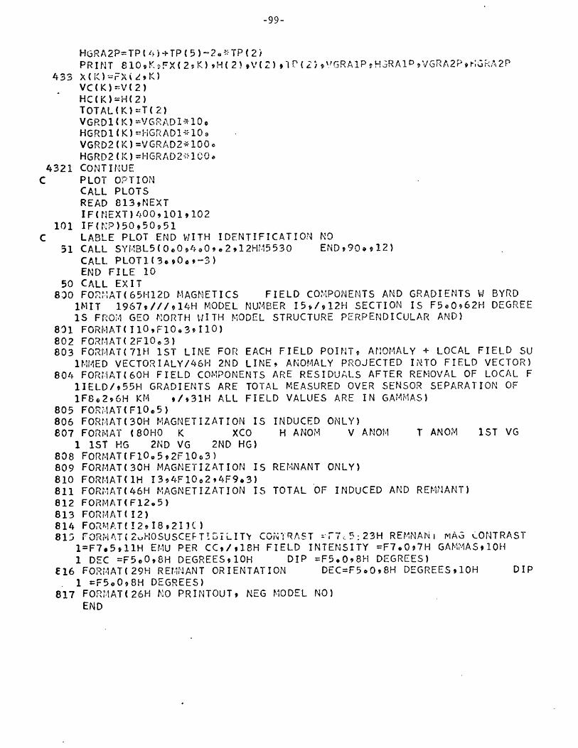
-99-
HGRA2P=TPt 4)+TP(5)-2. TP(2)PRINT 810,K FX(2sK) 9H( 2) ,V(2) #lP(2 ~VxGRA1P H3RAlPVGRA2Prr;G
433 X(K)=FX( K)VC(K) =V(2)HC(K)=H(2)TOTAL(K)=T(2)VGRD1(K)=VGRADl*10,HGRD 1K) HGRAD1 10,VGRD2(K)=VGRAD2 100oHGRD2(K)=HGRAD2-1'O.
4321 CONTINUEC PLOT OPTION
CALL PLOTSREAD 8139NEXTIF(NEXT) 4000 10 2
101 IF(NP)50950v51C LABLE PLOT END WITH IDENTIFICATION NO
51 CALL SYMBL5(0O,.a0 00, 212HM5530 END,90s1l2)CALL PLOT1(3oO0s,-3)END FILE 10
50 CALL EXIT8.0 FORIAT(65H12D MAGNETICS FIELD COPONENTS AND GRADIENTS W
IMIT 19679///14H MODEL NUMBER 159/,12H SECTION IS F5e062H1S FRO.I GEO NORTH WITH MODEL STRUCTURE PERPENDICULAR AND)
831 FORMAT(I1OFO,103oF10)802 FORMAT(2F10.3)803 FORMAT(71H 1ST LINE FOR EACH FIELD POINT, A'NOMALY + LOCAL F
1MMED VECTORIALY/46H 2ND LINE, ANOMALY PROJECTED INTO FIELD804 FORMAT(60H FIELD COMPONENTS ARE RESIDUALS AFTER REMOVAL OF
11IELD/v55H GRADIENTS ARE TOTAL MEASURED OVER SENSOR SEPARATI(
1F8296H KM ,/931H ALL FIELD VALUES ARE IN GAMMAS)
805 FORiMAT(FIOo5)806 FORMAT(30H MAGNETIZATION IS INDUCED ONLY)807 FORMAT (80HO K XCO H ANOM V ANOM T ANOM 1
1 1ST HG 2ND VG 2ND HG)808 FORMAT(F1I0.52F10o3)809 FORMAT(30H MAGNETIZATION IS REMNANT ONLY)
810 FORMAT(H 1394410o2 F9.3)811 FORMAT(46H MAGNETIZATION IS TOTAL OF INDUCED AND REMN-ANT)812 FORMAT(Fl2.5)813 FORMAT(12)814 FORMAT(12*189211()815 FORMAT%' 2UHOSUSCEFTIILITY CONTRAST 5F75:23H REMNANI MAG CO
1=F7.5llH EMU PER CC/9,18H FIELD INTENSITY =F7,?07H GAMMAS,1 DEC =F5.0,8H DEGREESslOH DIP =F5.0j8H DEGREES)
E16 FORMAT(29H REMNANT ORIENTATION DEC=F5.0,8H DEGREES,1OH1 =F50>O8H DEGREES)
817 FORMAT(26H NO PRINTOUT, NEG MODEL NO)END
A 2P
BYRDDEGREE
IELVECLOCON
ST VG
NPTRAST10H
DI
D SUTOR)AL FOF
P

-100-
C PLOT SU2JROUTINE FOR 2D MAG W BYRD MIT 15.1SUBROUTIZ PLOTSDI iiEN'S I C BUFIi G000) XAX I S ( 2),Y'?XIS(2) vAi )DIMENSION TOTAL(200),VGRD1(200),VGRD2(200) HGRD1(200)9HG.D2(200)gH
1C(200) VC( 200)(200 (200),X(200),EXX(200) ZEE(200)COMON TOTALVGRDIVGRD2,HGRD1,HGRD2,HCVCZsXEXXJTOTsKTOTIDENT
1 ,FDDIP,AJBACSUSoNPNEXTsZEEREAD 814,NPLOTNCOMIPgNVERNHORZIF (NPLOT)50095009501
501 CALL PLOTS1(BUF,1000)DO 502 J=1,JTOT
502 Z(J)=-ZEE(J)XAXIS( 1) =X(1)XAXIS(2) =X(KTOT)YAXIS'1)=0.YAXIS(2) =0,
C SET SCALES
S2=1.553=5eIF(S2+S3-95) 591,591,590
590 S2=955S2/(S2+S3)S3=9e5"S3/(S2+53)
591 IF(S1-10)5939592,592593 S1=1O592 CONTINUE
IF(NP)52095209510C LABLE GRAPH WITH IDENTIFICATION NO
520 CALL SYMBL5(0.0,4oO~*2,14HM5530 BEGIN 9Ooll-4)CALL PLOT1(3*9,0,-3)NP=1
C DRAW MODEL STRUCTURE510 CALL PICTUR(S1tS2,14HMODEL GEOMETRYt14,7HZ IN KMs79 EXXsZtJTOT,0oq0
1 XAXIStYAXISe 2,0 0)C DRAW SEA LEVEL AND OUTLINE DATA BLOCK
CALL PLOT1(-3.Oo93)CALL PLOT1(-3 S2+S3+o5,2)CALL PLOT1(-(S1+3o.)S2+S3+-5,2)CALL PLOT1(-(S1+3o) S2+5392)CALL PLOT1(-3,,S2+S3,2)CALL SYMBL5(-4.S2+*05tol9HSEA LEVEL,0.,9)CALL SYNBL5( -4 5,0591e17HW BYRD MIT 19670,,017)CALL P!LOT1( (143*)0o-3-3)
C WRITE DATA BLOCKCALL SYIBL5(0olS2+S3+.35,e1,5HMIODELOo,95)CALL NUMBR1( 65,S2+S3+.35.leIDENTOes,-0)CALL SYMBL5(S1-4o59S2+53+,35,,1,51HFIELD GAMMAS DEC
1 DEG DIP DEGoOog51)CALL NUMBR1(S1-3.80S2+S3+.35.1,Fo0.,0)CALL NUNBR1(S1-2,00,S2+S3+,35,.1,DOo ,0)CALL NU~,3R1(S1-o70,tS2+S3+o35,,,DIP,0 0)CALL SYMBL5(S1-4,5,S2+S34-+,2,o,ll8HSEC STRIKE DEGOa,18)CALL NUMBR1(S1-3.55 S2+S3+.2,1.Cs0.O 0)IF(AJ)51135129511
511 IF(SUS)51395149513

-101-.Li
512 CALL SYM~!( o5 5SSS3+.35e 1,26HINDUCED MAGNETIZATION ONLYo, 26)
517 CALL SY0i L5(S1-2 52+S3+o2o1,28HSUSCEPTILIBITY EMU/CCK0o.U128)CALL NUN BR1(S1-e20,52-S3+,2,1,SUS0.,5)GO TO 515
513 CALL SYr3L5(1659S2+S3+o35,ol,33HINDUCED AND REMNANT MAGNETIZATIONO10 ,33)GO TO 516
514 CALL SYMBL5(l5.-S2+S3+.359,lv26HREMNANT MAGNETIZATION ONLY06926)
516 CALL SYMBL5(SI-4.59S2+S3+.-oO5,o9,51HREM MAG EMU/CC DEC
1 DEG DIP DEGOoo51)CALL NUN38R1(S1-3o80,S2+S3+05eO.1AJ90.,5)CALL NUfBR1(S1-2*00S2+S3+059°1sBO)O)CALL NU-'iDR1(S1-,,70oS2+S3+.O5,1, A,Oo0)IF(SUS)517,5159517
515 IF(NCO-P)5039503i504503 IF(NVER)505,505,506505 IF(NHORZ)509o509q508
C PLOT TOTAL ANOMALYtHORZ AND VERTICAL COMPOENTS504 CALL SYM.BL5(Oo1,S2+S3+.2,21,55HMAGNETIC ANOIALIES, TOTAL HORZ AND
1 VERTICAL COiPONENTSo0.55)C LABLE INDIVIDUAL PLOTS WITH CENTERED SYM3OL AT MAX Y VALUE, T,VsH
CALL NIN{AX(TOTALtKTOTAMi(1)AMM(2))CALL MI N AX(VCKTOTAM1 (3) ,AMM (4) )CALL. MINtMAX(HC KTOT,A (5), A M (6)AMV41(7)=0sCALL DXDY1(AM,l79S39YMINDY,ND, KK)
CALL DXDY1(XKTOTS1,XMI N DX sNDsiKK)CALL MAX(TOTALtKTOTAMAXM)CALL SYFBL5((X () -XMIN)/DX (TOTAL(M)-YMIN)/DY+S2g.1951O9,a-1)
CALL MAX(VCKTOTqAMAX M)CALL SYtM3L5((XftlM)-XMIN)/DXs(VC(M)-YiIN)/DY+S2, a153,0.,-1)CALL MAX(HCKTOTAMAXqM)CALL SYN"L5( X(M)-XMIN)/DX,(HC(M)--YMIN)/DY+S2, 124,0, -1)CALL PLOT1(OaS2,-3)CALL PICTUR(S1,S3925HHORIZONTAL DISTANCE IN KMW2527HANOMALY MAGN
IITUDE IN GAMMAS,27,XTOTALKTOT,0,O0,XHCKTOTQo.0sXoVC.KTOT,0.901 XAXISYAXIS,290* 0)CALL PLOT1(0,t-S29-3)NCOMP=OIF(NVER)5189518,510
518 IF(NHORZ)509,509,510C PLOI 1OtAL 4NOMALY9 1ST AND 2ND vtRTICAL GRADIENTS
506 CALL SYMBL5(OolS2+S3+2,,1,58HMAGNETIC ANOMALIESs TOTAL, 1ST AND
1 2ND VERTICAL GRADIENTS0.,58)CALL SYMBL5(Os1,S2+S3+.05t,1,58H15T GRADIENT, 10X, 2ND GRADIENT, 1
100X VERTICAL EXAGERATION90o,58)C LABLE INDIVIDUAL PLOTS WITH CENTERED SYMBOL AT MAX Y VALUE, T,1*2
CALL MIN.IAX(TOTAL'KTOTAMtM(1),AMM(2))CALL MIN;MAX(VGRD19KTOTsA,'MM(3),AMM(4))CALL MINMAX(VGRD2 K TOTAM (5) ,AMM(6) )AM ( 7)=0CALL DXDY1(AMN,7,S3,YMINDY,NDKK)CALL DXDY1(XKTOTS1,XMINDXNDKK)CALL MAX(TOTAL9KTOTAMAX9M)

-102-
CALL SYML5 i i (M)-XMtIN)/DX9,(iO1ALi(',-YMiN)/PY+S2 a 9519,0 -1)CALL MAX(VGRDI,KTOTAMAX M)CALL SY; iL5((X(M)-XMIN)/DX 9 (VGR"D' : ) - ' N/DY52, 1%Ce-1)CALL MAX(VGRD29KTOTAMAXM)CALL SYMBL5((X(M)-XMIN)/DX(VGRD2(M)-YMIN)/DY+S2.ol 290*9-1)CALL PLOT1(0agS29-3)CALL PICTUR(S1S3925HHORIZONTAL DISTANCE IN KMf25#27HANOMALY MAGN
1ITUDE IN GAKMMAS27XTOTALKTOT.O7,0sXgVGRD19KTOT0Oo 0XVGRD29KTO1TO, >0,XAXIS9YAXIS)29q0 90)CALL PLOT1(0~-2S2-3)NVER=OIF(NHORZ)5099509o510
C PLOT TOTAL ANOMALY 1ST AND 2ND HORIZONTAL GRADIENTS508 CALL SYMBL5(OoltS2+S3+.29o1,54HHIAGNETIC ANO'ALIES9 TOTAL9 1ST AND
1 2ND HORZ GRADIENTS90.o54)CALL SYNI8L5(Ol1,S2+S3+e05,ol958H1ST GRADIENT, 10Xi 2ND GRADIENT, 1
10OX VERTICAL EXAGERATIONe0,58)C LABLE INDIVIDUAL PLOTS WITH CENTERED SYNSOL AT MAX Y VALUEs T91,2
CALL MINMAX(TOTAL KTOTAMM( 1) ,AMM(2))CALL MINMAX(HGRD1KTOT,AMi(3)tA-E'(4) )CALL MINMAX(HGRD2sKTOTAMM(5) AMM(6))AMM(7)=0OCALL DXDYI(AMM,7SS3,YMIN 9 DYoNDKK)CALL DXDY1(X9 KTOTS1gXMINDXND9 KK)CALL MAX(TOTALKTOTAMAXoM)CALL SY;4BL5((X(M)-XMIN)/DX,(TOTAL(M)-YMIN)/DY+S2,.195190s,-1)CALL MAX(HGRD1#KTOTAMAXM)CALL SYBL5((X(M)-XMIN)/DX,(HGRD1(M)-YMIN)/DY+529.1, 190,-1)CALL MAX(HGRD2oKTOTAMAXM)CALL SYMBL5((X(M)-XMIN)/DXo(HGRD2(M)-YMIN)/DY+S29.19 290,-1)
CALL PLOT1(0*sS29-3)CALL PICTUR(SIS3925HHORIZONTAL DISTANCE IN KM,25927HANOMALY MAGN
1ITUDE IN GA.MAS279XTOTAL,KTOT,0.0,XgHGRD1,KTOT,00 .OX.HGRD2,KTO1Ts90oe0XAXISYAXIS9290e90)CALL PLOT1(Oo-S2,-3)NHORZ=0
509 CONTINUE500 RETURN814 FOR4AT(I2,I82110)
END

-103-
C SJUBKOUTIiE* TO FINL IAX ELEMIENT OF 10 ARRAY W BYRD MIT 1967C A IS ARRAY NAMEe KTCT IS NO OF ARRAY ELEMENTS AMAX IS VALUL uFC MAX ELEMENT, M IS SUBSCRIPT OF AMAX
SUBROUTINE MAX(AKTOTAMAXM)DIMENSION A(200)AMAX=0.DO 1 K=1KTOTIF(AMAX-A(K))2 91
2 AMAX=A(K)M f
1 CONT INUERETURNEND

-1011-
C DUI",,y PLOTS SUBRCUTINE Wh BYT'kD tM-IT 3j-67SUS{,BROkTjIN,1- PLOTSREAD~~4~P T;~cMVR~>'2RET URN
814 FOZlMAT( X2q18o2I 10)E ND
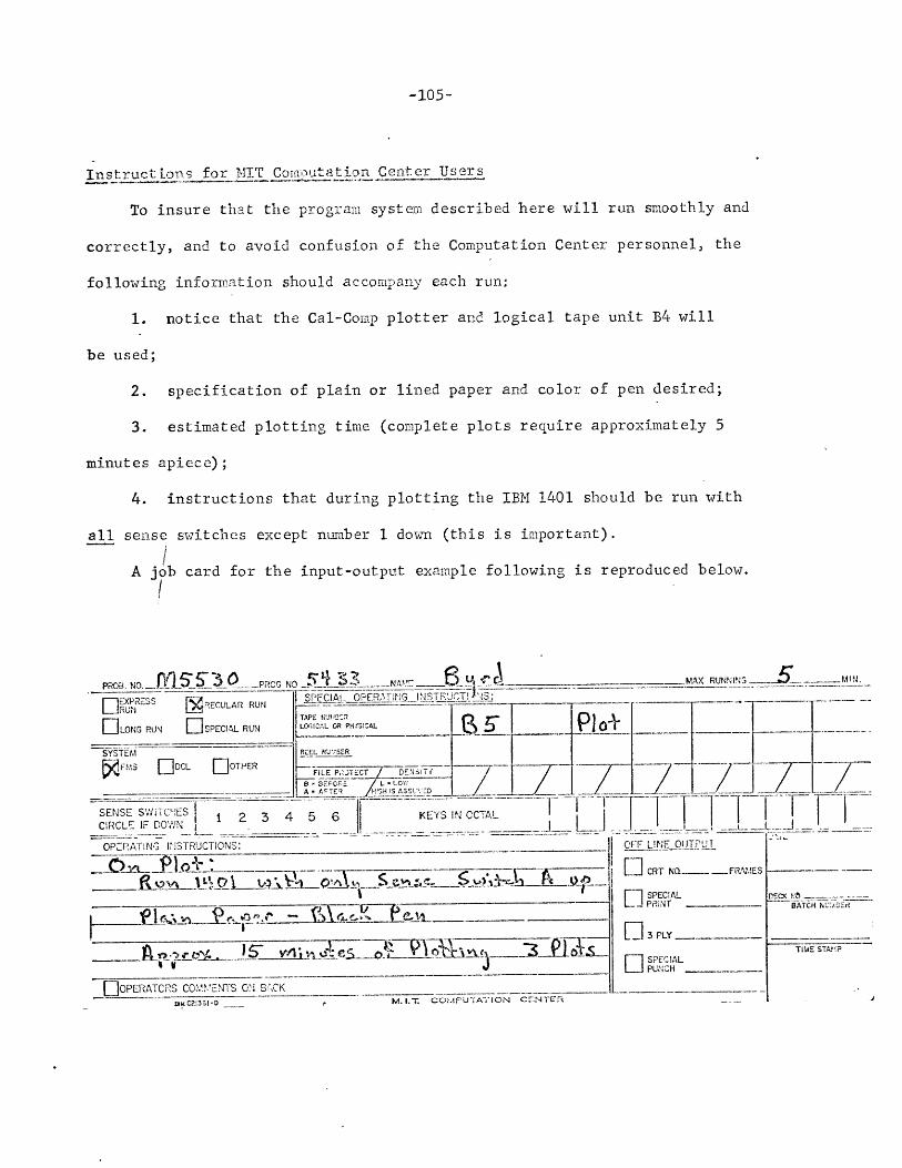
-105-
Instructions for MIT Com-outation Center Users
To insure that the program system described here will run smoothly and
correctly, and to avoid confusion of the Computation Center personnel, the
following information should accompany each run:
1. notice that the Cal-Comp plotter and logical tape unit B4 will
be used;
2. specification of plain or lined paper and color of pen desired;
3. estimated plotting time (complete plots require approximately 5
minutes apiece);
4. instructions that during plotting the IBM 1401 should be run with
all sense switches except number 1 down (this is important).
A job card for the input-output example following is reproduced below.
PROB. NO. PROG NO _3 NAM ______ __ _ _ MAX RUNNING- - MgN
RECULAR RUN SPECIAL OPERMING INSTRCT!-
RULONG RUN ISPECIAL RUN
SYSTEM REL NL;"RER
CIRCLE IF EOWN WN _ _ __ ___ ___L i . . . ... . . . . .
___ _,_ - CRT NQ FRN.ES - __-.3 SPECIAL DECIDL OTER
PRiNT - BATCH LO ,ERSENSE S[3PY TC-ESlYC L F _ _ . .._-KEYS IN CCTATI STA
-. . . J _SPECAL_
]OPERATCRS COMIENTS O. B iCKai213I-0 M.I.T. COIPUTATION CENTE R
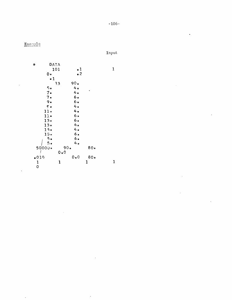
-106-
Input
* DATA101 .1 1
0. .2.1
rs 421.3 90,
7. 4.7. 6.9. 6.
11. 4,11* 6.13* 6.13. 4,15* 4.15 6.5o 6.
15, 4.
50000. 90. 80.1 0.0
.010 0,0 80.1 1 1 10
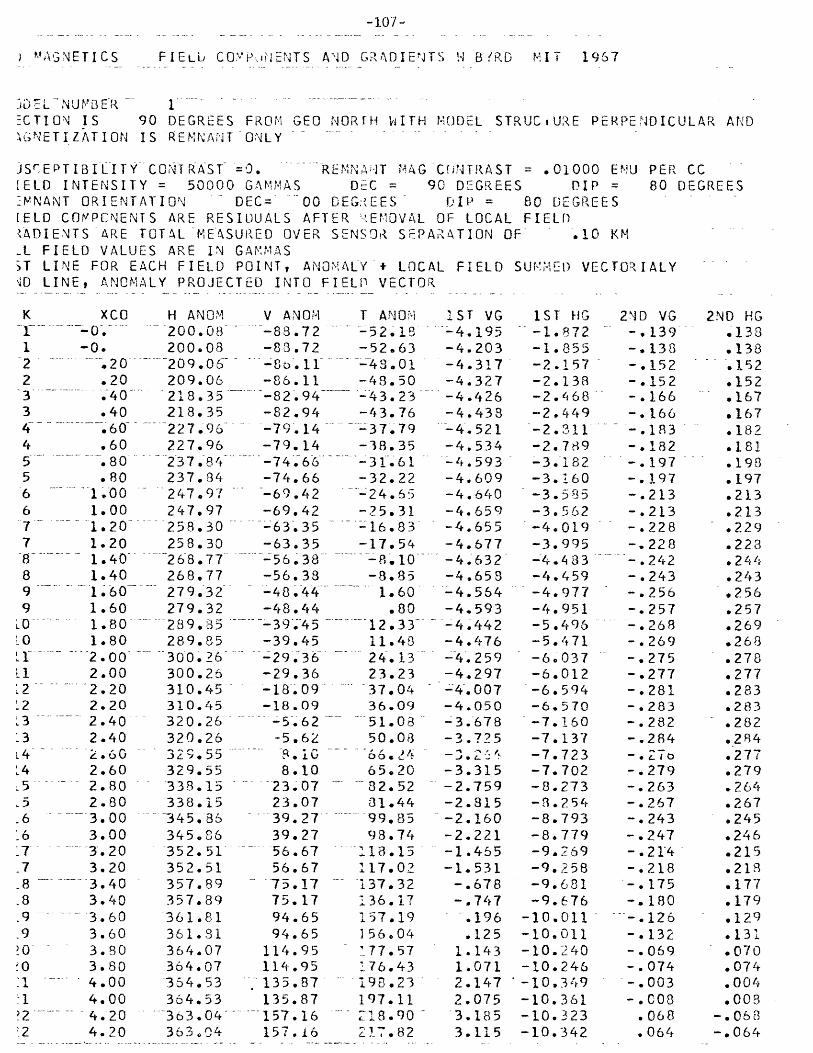
-107-
A RAGNETI CS
]DCL-NUMBERECTION IS
GNET I ZAT I ON
FIELL COYP 'ENTS AND GRADIENTS t' BRD MIT 1967
90 DEGREES FROM GEO NORTH VITH MODEL STRUCI:URE PERPENDICULAR ANDIS REMNANT ONLY
JSrEPTIBILITY CONTRAST =O. REMNANT MAG CfNTRAST = .01000 ENIU PER CC[ELD INTENSITY = 50000 GAMMAS DEC = 90 DEGREES DIP = 80 DEGREESIMNANT ORIENTATION DEC= 00 DEGREES DIP = 80 DEGREESIELD COMPCNENTS ARE RESIDUALS AFTER EMOVAL OF LOCAL FIELD,ADIENTS ARE TOTAL MEASURED OVER SENSOR SEPA,RATION OF .10 KM-L FIELD VALUES ARE IN GAMMAS3T LINE FOR EACH FIELD POINT,'0 LINE, ANOMALY PROJECTED IN
ANOMALY + LOCAL FIELDTO FIELD VECTOR
SUMMED VECTORIALY
K XCO
1 -0.2 .. -202 .203 .40-3 .404 .604 .605 .805 .806 1.006 1.007 1.20-7 1.208 1.408 1.409 1.609 1.60
1L .... . 1.80LO 1.80L1 -.. . 2.00L1 2.00
2 2.2012 2.2013 - 2.40,3 2.40
14 2.60,5 - 2.80.5 2.80.6 3.006 3.007 3.20
.7 3.20
.8 3.40
.8 3.40,9 3.609 3.60
)-0 3.80'0 3.801A 4.00
:I 4.00. 4.20
2 4.20
H ANOM200.08200.08.209.06209.06218.35218.35227.96227.96237.84237.84247.97247.97258.30258.30268.77268.77279.32279. 32289.35289.85
. 300. 26300 .25310.45-310.45320.26320.2632). 55329.55338.15338.15
-345.86345.86352. 51352.51357.89357.89361.81361.81364.07364.07354.53364.53
- 3603.04'363 .04
V ANOM-88.72 -
-88.72-8 .11-86.11-82.94 .--..-82.94-79.14 ...-79.14-74.66-74.66-69.42-69.42-63.35-63.35-56.38-56.38-48.44-48.44-. 39.45
-39.45-29.36-29.36-18. 09-18.09-5.62-5.62
8.10.23.0723.07
....39.2739.27
-5 6 . 6756.67
- 75.1775.1794.6594.65
114.95114.95135.87135.87157.16157. 16
T ANOM 1ST VG-52.18 -4.195-52.63 -4.203-43.01 - -4.317-48.50 -4.327- 43.23 .- 4.426-43.76 -4.438-37.79 -4.521-38.35 -4.534-31.61 -4.593-32.22 -4.60924.65 -4.640
-25.31 -4.659-16.83 -4.655-17.54 -4.677-8.10 -4.632-8.85 -4.658
1.60 -4.564.80 -4.593
12.33 -4.44211.48 -4.47624.13 -4.25923.23 -4.29737.04 -4.00736.09 -4.05051.08 -3.67850.08 -3.72566.4 -3.25 -65.20 -3.315
-82.52 - -2.75931.44 -2.81599.85 -- 2.16098.74 -2.221
118.15 -1.455117.02 -1.531137.32 -. 678136.17 -. 747157.19 .196156.04 .125177.57 1.143176.43 1.071198.23" 2.147197.11 2.075
198.90 3.185217.82 3.115
IST HG-1.872-1.855-2.157-2.138-2.4 68-2.449-2.311-2.789-3. 182-3.160-3.585-3.562-4.019-3.995-4.433-4.459-4.977-4.951-5.496-5.471-6.037-6.012-6.594-6.570-7.160-7.137-7.723-7.702-8.273-8.254-8.793-8.779-9.269-9.258-9.681-9.676
-10.011-10.011-10.240-10.246-10.349-10.361-10.323-10.342
2ND VG-. 139-. 138-. 152-. 152-. 166-. 166-.183-. 182-. 197-. 197-. 213-. 213-. 228-. 228-. 242-. 243-,.256-. 257-. 268-. 269-. 275-. 277-. 281-. 283-. 282- .284
-. 279-. 263-. 267-. 243-. 247-. 214-. 218-. 175-. 180-. 126-. 132-. 069-. 074-.003- .008
.068
.064
2ND HG.138.138.152.152.167.167.182.181.198.197.213.213.229.223.244.243.256.257.269.268.278.277.283.283.282.284.277.279.264.267.245.246.215.218.177.179.129.131.070.074.004.008
-. 068-. 064
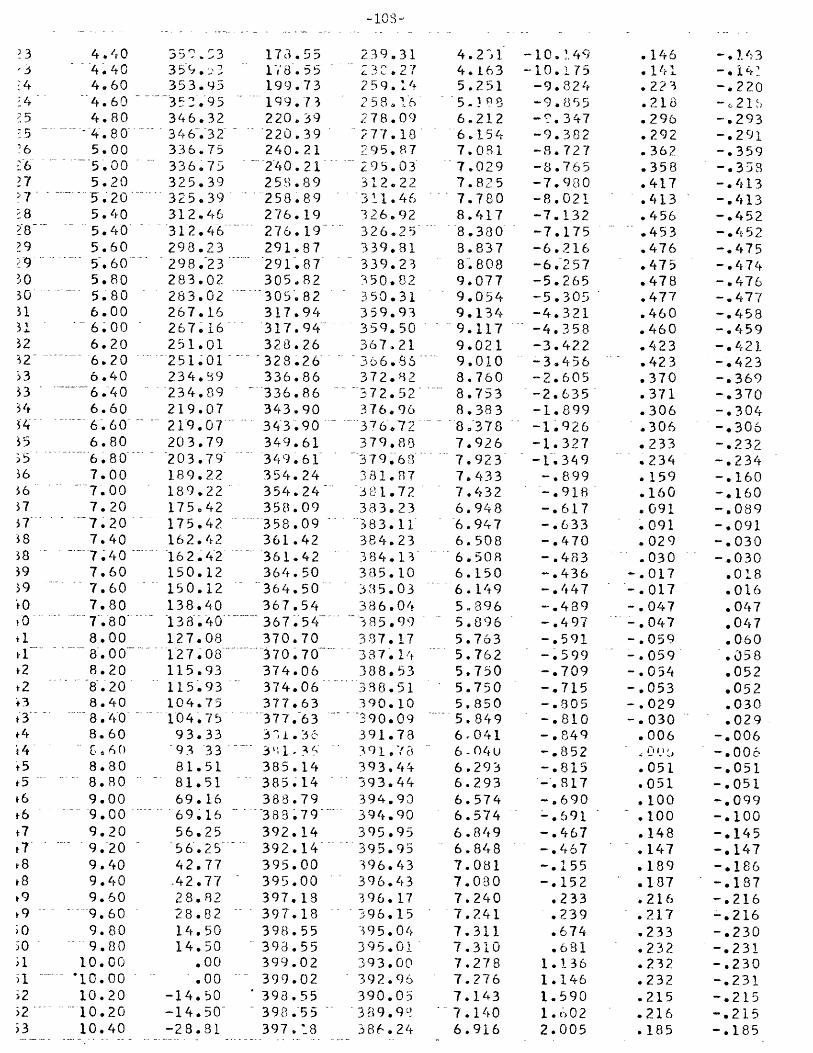
-10S-
13 4.40,3 4.404 4.60
.4 4.6015 4.80
5 .4.806 5.00
_6 .5.007 5.207 ' 52018 5.4018 5.4019 5.60_9 5.6030 5.8030.. 5.8031 6.00
.31. 6.0032 6.2012 6.205'3 6.4033 6.4034 6.60
: . . .6.6015 6.805 .6.80
36 7.0056 7. 0017 7.2057 - 7.2038 7.408 7.40
39 7.609 . 7.60O 7.80
t-0 ---.--.. ... T .8 0+1 8.00I 8.00-t2 8.20t2 8,20+3 8.40t3 ... 8. 40,4 8.60
15 8.80t5 . . 8.80t6 9.00'i6 . 9.00t7 9.20t7 9.20k8 9.40t8 9.409 9.609 .. . 9.60
)0 9.8050 . . 9.8031 10.00)1 . 10.00-)2 10.202 .. 10.20
)3 10.40
35,53359.,23353.9535..95346.32346 . 32-336.75336.75325.39325.39'312 • 46312.46
298.23298.23283.02283.02267.16267.16-251.01251.01234.9234.89219.07219.07203.79203.79189.22189.22175.42175.42162. 42162 42150.12150.12138.40138. 40127.08127 08115.93115.93104.75S104.75
93.3393 33 -
81.5181.5169.1669.1656.2556. 25---42.77.42.7728.8228.8214.5014.50
.00
.00-14.50-14.50-28.81
178.55 239.31178.55 23c.27199.73 259.14199.73 258216220.39 278.09220.39 277.18240.21 295.87
...2-40.21 295.03258.89 312.22
..258.89 311.46276.19 326.92276.19 326.25291.87 339.81291.87 339.23305.82 350.82305.82 350.31317.94 359.93317.94 359.50328.26 367.21328.26' 306.86336.86 372.82
-336.86 -3 72.52343.90 376.96343.90 376,72349.61 379.88349.61 379.63354.24 381.87354.24 3 1I.72358.09 333.23358.09 383.11361.42 384.23
-'..361.42 . 384.13-364.50 385.10364.50- 335.03367.54 386.04367.54 385.99370.70 387.17370.70 38 7 .elt374.06 388.53374.06 338.51377.63 390.10.377.63 . .390.093"1.36 391.73
-. 381-3' 39 .78385.14 393.44385.14 393.44388.79 394.90
. 38-3.79 ...... 394.90392.14 395.95392.14 395.95395.00 396.43395.00 396.43397.18 396.17397.18 396.15398.55 395.04393.55 395.01399.02 393.00399.02 392.96398.55 390.05398.55 389.9?)397.18 386.24
4.2314.1635.251
6.2126.1547.0817.0297.8257.7808.4178.3808.8378.8089.0779.0549.1349.1179.0219.0108.7608.7538.3838. 3787.9267.9237.4337.4326.9486.9476.5086.5086.1506. 1495.8965.8965.7635.7625.7505.7505.8505.8496 0416-04u6.2936.2936.5746.5746.8496.8487.0817.0807.2407.2417.3117.3107.2787.2767.1437.140
-10,. 149-10.175
-9.824-9.855
-9.347-9.382-8.727-8.765-7.980-8.021-7.132-7.175-6.216-6.257-5.265-5.305-4.321-4.358-3.422-3.456-2.605-2.635-1.899-1.926-1.327-1.349
-. 899-. 918-. 617-. 633-. 470-. 483-. 436-.447-. 489-. 497-. 591-. 599-.709-.715-. 805-. 810-. 849-.852-. 815-. 817-. 690-. 691-. 467-. 467.155
-.152.233.239.674.681
1.1361.1461.5901 . 02
6.916 2.005
.146
.223
.296
.292
.362
.358
.417
.413
.456
.453
.476
.475
.478
.477
.460
.460
.423
.423
.370
.371
.306
.306
.233
.234
.159
.160
.091
.091
.029
.030
.017
.017
.047
.047
.059
.059
.054
.053
.029
.030
.006
.051
.051
.051
.100
.100
.148
.147
.189
.187
.216
.217
.233
.232
.232
.232
.215
.216
-. 143-. 141-. 220- 21-. 293-. 291-. 359-. 353
-. 413-. 413-. 452-. 452-.475-. 474-. 476-. 477-. 458-. 459
-. 421-,423
-. 369-. 370-. 304-. 306-. 232-. 234-. 160-. 160-. 089-. 091-. 030-. 030
.018
.016
.047
.047
.060
.058
.052
.052
.030
.029-. 006-. 006-.051-.051-. 099-. 100-.145-.147-. 186-. 187-. 216-. 216-.230-.231-. 230-. 231-. 215-. 215
.185 -. 185

-109-
'3 10.4054 10.6054 10.6055 - 10.8055 10.8056 11.0056 11.0057 11.2057 11.20580. 11.4058 11.4059 .- 11.6059 11.6060 11.8060 11.8061 - 12.0061 12.0062 12.2062 12.2063 12,4063 12.4064 12.6064 12.6065 12.8065 12.8056 . 13.0066 13.0067 13.2007 13.2068 13.4068 13.4069 13.6069 13.6070 13.8070 13.8071 14.0071 14.0072 .. ..14.2072 14.2073 14.4073 14.4074 . 14.6044 14.6075 14.8075 14.8076 15.0076 15.0077 15.2077 15.2078 15.4078 15.4079 15.6079 15.6080 15.303 0 15.30
dl 16.0081 16.0032 .16.2082 16.2083 .---.- ' 16.-4083 16.40
-28.8 1-42.77-42.77-56.25-56.25-69.16-69.16-81.51-81.51-93.33-93.33
-104.75-104.75-115.93-115.93-127.08-127.03-138.40 -
-138.40-150.12-150.12-162.42-162.42-175.42-175.42-189.22-189.22-203.79-203.79-219.07-219.07-234.89-234.89-251.01-251.01-267.16-267.16-283.02-283.02-298.23-298.23-312.4'-312.46-325,39-325.39-336.75-336.75-346 . 32-346.32-353.95-353.95-359.53-359.53-363.04-363.04-364.53-364.53-364.07
-364.07-361.831-361 8~1
397. 18315.00395.00392.14392.14388.79383. 79385.14385.14
. 381.36381.36377.63377.63374.06374.06370.70370.70367.54367.54364.50364.50361.42361.42353.09358.09354.24354.24349.61349.61343.90343.90336.86336.86328.26328.26317.94317.94305.82305.82291.87291.87276.19276.19-:3 . 89258.89240.21240.21220.39220.39199.73199.73173.55178.55157.16157.16135.87135.87114.95114.9594.6594.65
386.14331.6931.57376.57
376.42371.05370.83365.35365.13359.61359.36353.99353.71348.56348. 25343.36343.00338.32337.93333.34332.90328.22327.73322.73322.18316.61316.00209.59308. 91301.39300.63.91.78290.95280.60279.68.67.72266.72253.12252.02. 36.83235.65218.99717.7319 ' II
q198.46179.47178.03158.34156.90136.70135.24. 14.89113.4193.2191.7371.9770.5151.4249.9931.7730.33
6.9136 .bLO
6.6156.2056.2785.9415.9345.6275.6195.3755.3655.2115.2015.1555.1465.2165.2065.3895.3795.6605.6496.0015.9916.3816.3676.7566.7407.0857.0667.3277.3037.4457.4157.4107.3737.2027.1586.8146.7626.2496.1895.5215.4534.6544.5793.6783.5982.6282.5441.5411.455
.454
.366-. 604-. 689
-1.601-1.634-2.517-2.595-3.335-3.408
2.0182 3542.3702.6212.6362.7922, 8082.8692.8852.3622.8782.7912.6082.69342.7032.5772.5962.5022.5232.4972.5202.5902.6162. 3062.8343.1553.1873.6443.6794.2614.3004.9895.0305.7995.8426.6546.6987.5177.5618.3478.3899.1049.144
9.79210.28010.30810.65010.67110.86010.87410.90910.91410.8 0110.79810.55010.54110.17510.1599.6969.674
.14-
.145-, 009
.098.050.050.006.006
-. 029-. 029-. 050-. 051-. 057-. 056-. 043
-. 043-. 014-. 013
.034
.033
.091
.093
.159
.159
.228
.229
.295
.295
.353
.354
.398
.398.428.426. 436.434.424.421.393.390.344.340.281
.276
.208
.202
.127
.122
.046
.040-.032-. 039-. 106-. 113-. 172-. 177-. 227-. 231-. 271-. 275
-,1r63
-. 145
-.098-. 098-. 050-. 050-,005-. 006
.029
.029
.051.050.055.055.044.043.013.013
-. 032-. 034-. 090-. 092-,157-. 160-. 228-. 229-. 294-. 295-. 353-. 353-. 397-. 398-. 424-. 425-. 434
-. 433-. 421-. 421-. 391-. 389-.343
-. 219-. 276-. 205-. 202-. 125-. 121-. 044-. 040
.036
.039
.108
.112
.171
.176
.228.231.272.275

U4858586868787888889399090919192929393949495959696979798989999
000001
16.60 -357.89 75.17 3.2116.6C -357.89 15.17 11.8816.80 -352, 1 56.67 -4.1316.80 -352.51 56.67 -5.4117.00 -345.86 39.2( -20.1717.00 -345.86 39.27 -21.3"'17.20 -338.15 23.07 -34.8617.20 -338.15 23.07 -36.0017.40 -329.55 8.10 -48.1917.40 -329.55 8.10 -49.2517.60 -320.26 -5.62 -50.1517.60 -320.26 -5.62 -61.15
17.80 -310.45 -18.09 -70.8117.80 -310.45 -18.09 -71.73
18.00 -300.26 -29.36 -80.2118.00 -300.26 -29.36- . - 81.0518.20 -289.85 -39.45 -88.41...18.20 -289.85 -39.45 -89.1918.40 -279.32 -48.44 -95.5018.40 -279.32 -48.44 -96.2118.60 -268.77 -56.38 -101.5518.60 -268.77 - 56.38 -102.2018.80 -258.30 -63.35 -106.6518.80 -258.30 -63.35 -107.2419.00 -247.97 -69.42 -110.89
19.00 -247.97 -69.42 -111.4219.20 -237.84 -74.65 -114.3419.20 -237.84 -74.66 -114.8319.40 -227.96 -79.14 -117.08
19.40 -227.96 -. -79.14 -1 17.52
19.60 -218.35 -82.94 -119.1919.60- -218.35- -82.94- -119.5919.80 -209.06 -86.11 -120.74
19.80 -209.-06 -86. 11 -121.10
20.00 -200.08 -88.72 -121.79. 20.00 -200.08 -88.72 -122.12
-4.0" 5-4. 113-4.645-4. 7 r
-5.132-5.187-5.514-5.561-5.794-5.836-5.935-6.021-6.094-6.125-6.135-6.160-6 . 114-6.135-6,043-6.061-5.933-5.947-5.790-5.800-5.620-5.629-5.433-5.440-5.233-5.238-5.024-5.027-4.810-4.812-4.596-4.596
9.1359.1078.5138.4327.854
7.8207.1737.1386.4916.4545.8185.7815.1665.1304.5434.5093.9573.9233.4093.3772.9022 . 8722.4382.4092.0151.9881.6321.6081.2881.266.980.960.708.589.465.449
-. 30-. 326-- 3 )
-. 337-. 340-. 342- .343
-. 337-. 339-. 329-. 329-. 313-. 315
-. 298-. 298-. 278-. 278-. 257
-. 257-,237-. 237-. 216
-. 215-. 195-. 195-. 176-. 175
-. 159-. 157-. 141-. 140-. 124
-. 124-. 110-. 109
*3?5.328.338.339.340.342.338.339.328.329.315.315.297.298.279.278.259.258.237.236.216.216.196
.195
.177
.176
.158
.157
.140
.140
.125
.124
.109
.109

MODEL. REMNRNT MRGNEIIZRITIN ONLYMRGNETIC RN3MRL.IES, TOTRL, -HOf1RZ RND VERTICRL COMPONENTS
FIEL.D 50000SEL STRIKE 90REM MRG .01000
SER LEVEL
HORIZONTRL DISTRNCE
W BYRD MIT 1967
6.'o 80 100 12-0 1.0 15.0MODEL GEOMETRY
18.0
&R11MRSEG/C
EMU/CE
2.0
IN KM
4.0

MODE1L 1 f[1'1t'RNT rRrElRlU ONLYM1RGNET1f- RNOMRLIE5. 70TRL.,. 15T RNO 2ND V[E51[CL G13901[NT515T GERDIENT. IOX, 2ND 5RDINT. 1QOX V9TIuRL EXRG1f-.9,TIUN
FIELD t500005EC !3T9JK 90f95ri riR- -oi1000
Lj.Q 8.0
[lO I ZONTRiL10.0 12.0DISTRNCE IN KM
w ayif9O M I T 1967
MODiEL GELIME1 BY
EMU/CC
2.0 16,0 Ia10
7
20104.0
I
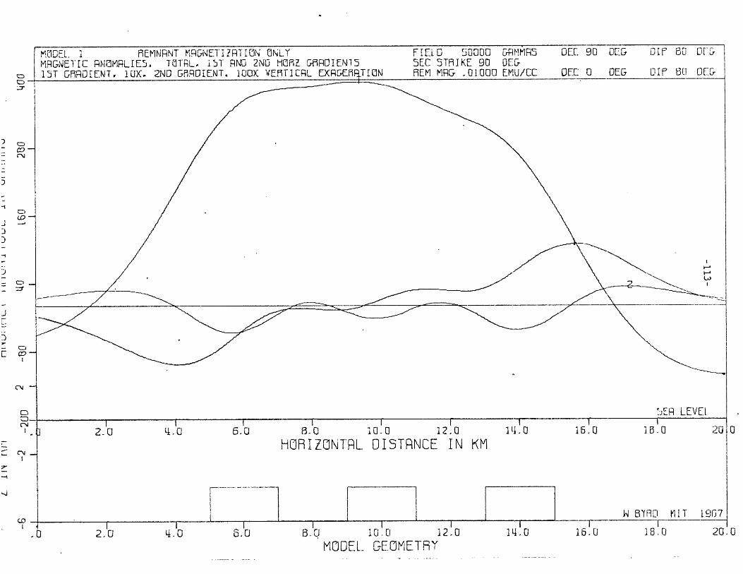
MODEL. 1 REMNRNT MFRNETIR1' T10f ONLY F EL 0 5000 OO gMMRS DEC: 90 OEG DIP 80 DEIMRGNETIC RMALIES,. TTARL. i5T RND 2ND !H0Z GfROIEN15 SEC STRIKE 90 0DE:-15T GRROIENT, 10X. 2ND GfRDIENT. 100X VETIARL EXRCF_~PPTON REM MRG .01000 EMU/CC DEC 0 OEG OLP 60 OEIr
CN
_____ E9 LEVEI
I 2.0 4.0 5.0 8.0 10.0 12.0 1t,.0 16.0 15.0 20 0HORIZONTRL DISTRNCE IN KM
W BRD M IT 1957IT
.0 2.0 4.0 6.0 B.10 .0 12.0 114.0 16.0 18.0 20.0
MODEL GEOMETRY

-114-
Appendix 2
ADDITIONAL COMPUTER MODELS

MIOEL. 1 REM9 NTMRGNETIC R fUMPLrE(, TrJTI
4fZ, CI I ZRTON ONLY. HCf.1liZ RND VERTICRL CUMPONENlNi
FIELO 30000 GMMRS DEC 0 --EG DiP 0 0CESEC T R IKE 45- 5DE EREM M5 01000 EMJ/ DEC 0 DEG D P 0 OEG-
1.-
/j7I
/ I, I
/ /
5ER LEVEL t/I I I
I I I8.O 10.0 12.0
HOFjiTZ NR 0 OISRiC,.E IiN KM
I I8.0 .. 10.0 1
FMODEL C-EOIME RY
I r.1 j -.
2.0i2.0
I16,0
I1..0
18.0 i20 i
N BYRDo MIT 1967
38.0 20.0
~.~~1
I2.0
I4.0
-ii
CI
I6.0
I6.02.0
- --
' -- ---
I I I
I ~'j I i
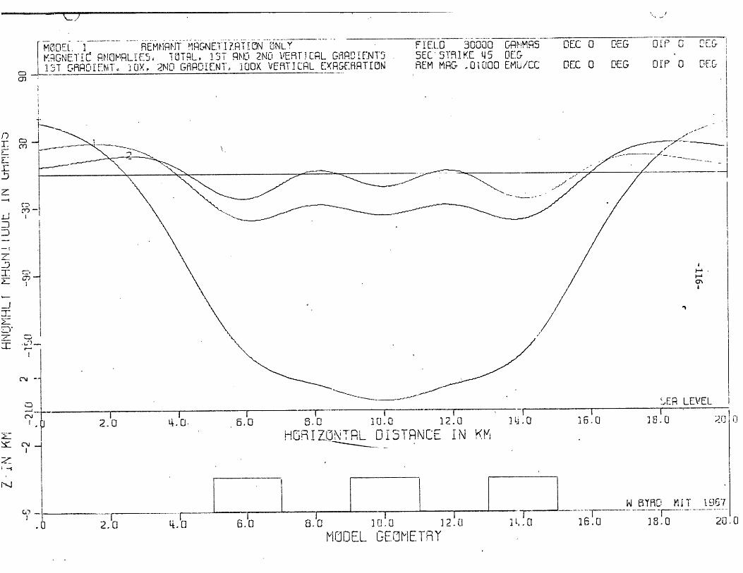
MOICIL. I REMIRM' MIRN[TI'?.R9TONI ONLY ~ F I EL 30000 &RNMRSVqGNETI-r RNOMRLIES, WT-RLP- I'-T RNICO 2N!,-. VE,9FjCRL GDR-"NIT.r 5EC '3Th1k' Li5 DCC
2 G 1RCIEN T OWX. 2ND Gi9R-'YENT :IO.V -~r-L [XR&C-H~RTEON Fi[M MP., .01000 EMUCC
~1
Th
CC 0 DC-
Cs C 0 D'EG
D 11F 0 rDE C-
DIP' 0 0 F-
110.0MIUDEL GEOMETHY
C7%1
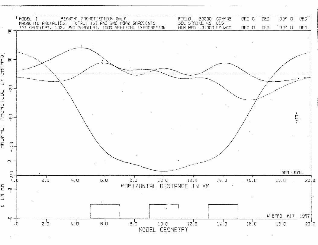
MqIGNETTC iML5.TUTPL,. 'I'T RNIO- 2N'\-2 HOi?. G-HPIO.IFIMT3KI T- HfP~NT A. UX 2'c GHCfTII0VE~rTrORL EX&9T.N
F I A.0 300005EC 5T1-91O 45HEfM M~rGl .wi1j00
DEC '0 C,~ Dr, C2, 0 lUEC 0 DES El F 0 E 51
EMIJ, /CC
8.0 10 0 122aHO'9IZUNTRL DISTRIEI~~
.25.0
5 EP L EVEL
N BYR3O ti IT 9C (7
Vc5DEL . EOMEPL.FY2.0
"-c t 0

MOEL 3 REMNRNT MRGET]ZRTION ONLYMRGNETIC RNOMRLIE, TOTRL, HORZ RNO VERTICRL COMFONENTS
FIELO 50000 GRMMRSSEC STRIKE 90 DEGREM MRG .01000 EMU/CC
HORIZONTRL
HDISTRNCE IN KM
w BT.D M iT 1967
80 90 100
MODEL. GEOMETRY
I_ i r vl 1 • •
,,
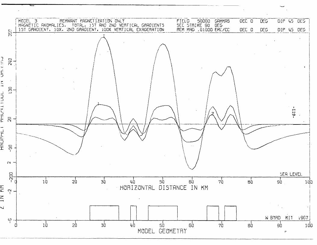
MieOEL 3 REMNNT MRGNETIZRTTIN OLY FIELD 50000 GRMIRS DECC 0 DEG DIP 45 DEMqGETIC RNIM.LIES, TITRL, ]ST RNO 2ND VERTICRL GRDIENTS SEC 5TRIKE 90 DEGTST GBRDI[ENT. 10X, 2ND GRROiENT, 100X VERT.CREL EX.RGERTION BEM MRG- .01000 EM/CC OEC 0 DEG DIP 4'5 DOE
/
/
OER LEVEL.
0 20 30 40 50 60 70 80 90HORIZONTRL DISTRNCE IN KM
W BTRD I T t967
50MODEL GEOMETRY
70
0
0
-Io i
J --133
-r7
~ r~
- -- I ---- --- -- ---- I -
---------
--
I
I
i
10
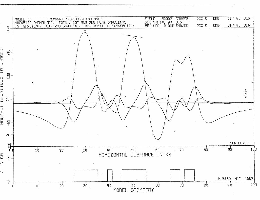
MODEL 3 REMNRNT MRGNETIZRTION ONLYMRGNETIC RQOML-IE5, TOTRL, 15T RND 2NO HORZ GF-9IROENTS1ST GfRDIENT, 1OX, 2ND G9qDIENTr IOOX VERTILRL EXR5ERTION
FIELD 50000SEC STR!KE 90REM MFRG .01000
GRMM S 5OEOrElf.U/CC
Do P 45 OEr
DOEC 0 DEG DIP l5 OE-
SER
HORIZONTRL DISTRNCE
N BYRD MiT
50
MODEL. GEOMETRY
IN KM
20
-liECFliP~-~- -- 1 II-
r;

MODEL 49EIWRNT MANEI*1 RT!N OJNL'
MW E T f C R RL I 'L7 5 TUTIL. tll Z rRNO VrEWF1TCrrL CCtOPONEFTELO 500co0SiEC~ c-TJE 90;I9M MRS,- 0 1 000
GRIMRSOC;
DECGD c I
rEC 0 DEG olp '45 0 E
Mfr.L
C 2. 1 '-L 5.0cI I I
10.0c 12.0HO I ZO~ L 0 .1 '3 1 ,]C E IN K V
II I-l 16 -G .0 20
-l 2.0 4-
MODEL GEOMVETH1Y
~TH0?M IT197
1~-0 20.0
t (~1
CN
'J L F-V[L

MOL 4 flErN.RNT tARr0,NETU,'HT.1N ONLYrh9GE1h~Nt{LWLTrJTPL., 15T RNOL' 2NL'J VE9TIC2L GRFIP.NT5.
I mT C - NT. 'IX,. 2ND GFI%'DYENT, "FO.V.~1L iffTrJ
LOl~
-9,1 l.u 5UUUUSEC S3T91KE 9093EI MRC .0100
r~A1H~jor
OEC 0 0EG7 FJl> 'V DE
DEC: 0 (0E~ G' k5 . IU;
c-'J -,
2.u
/ ~
4.o 5.0
c-'J~J
2.0 4.0
910
H F517 0N T PL10.012.0U
q 5TN r-,E I N K viI t .0 16. u
6 5.0
2
V{IiLL C&EYET9Y
9 6
5U LVEF) 0
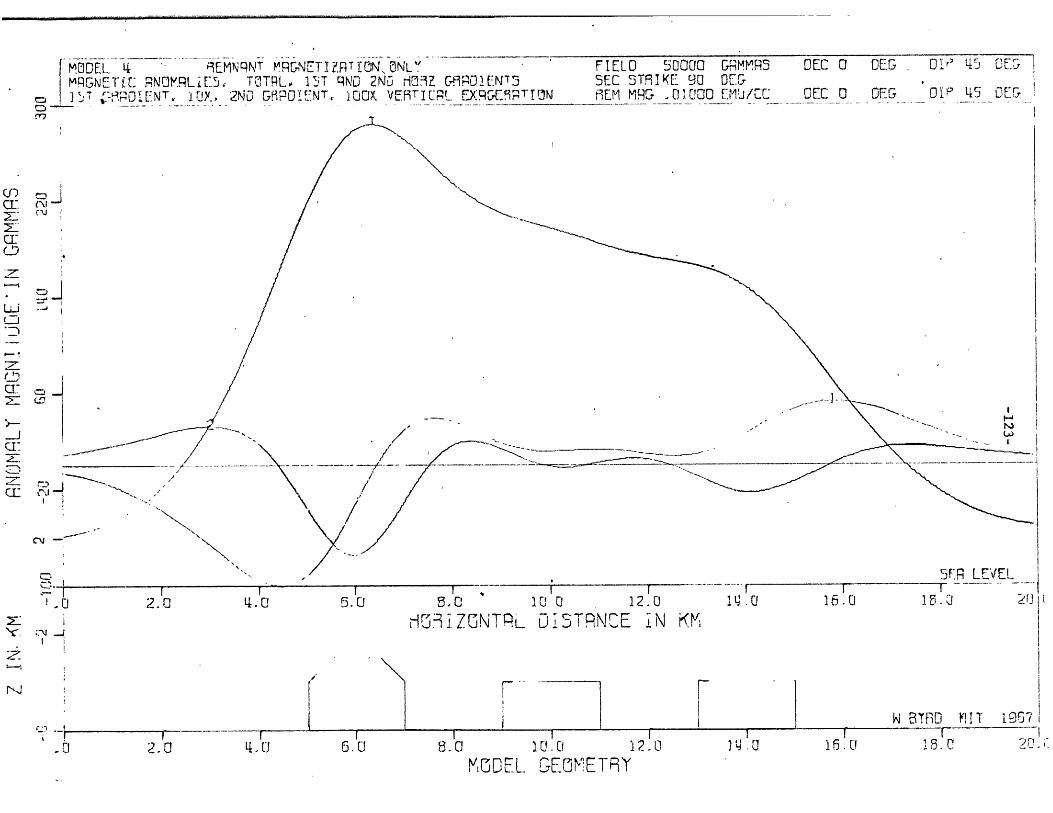
M1ODEL ---4 9 MN%9NT P R E T IR T 1.N, 0NL FIELD ~500RMMRS O 0EC 0lmq~T TO 2c.LL5 TjTRL 1-JT RNO 2ND0 Hri-Z CH"DEN75 SEC 5i1911(E 90x 0I
~ 3~T -j -NT,. iuJX, 2ND (,FpojrfNT. 1C00)( Vf. EmR :R rt4 _Mq .uoo w/cor
e-"
DEG DO 45 0oC
QEG OV ~5 QE
IH
Lk)
/ _
/
S/ /
7 U ,TQ IU Cl 12.0lDI5TN E I N
3t4
I6.
I INw B8.-0
V,3DE1Lr GEOMET-nrYi2 16. - I
5F1R LF VEIL
TFD N1T 19G-1
20,~i
U 2. 0 ~5. U
1V -9
2.01 6.0cl
f.
I q , cl1
4.0
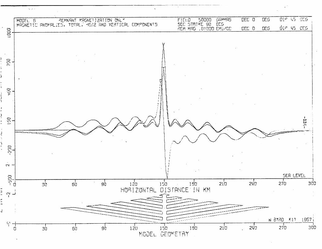
MODEL 5 ,EMNqNT QRGNE'fITZRTr1N ONLY FIFt. 50000 r1rS5 OEC 0 E D 0DI p 5 DF1
MqrGNEIC PN~,'9L;:;5, TOTL. 0;ILZ RN VERTICPL C',KPOiNENT 5EC STKE 90 OEG_REM __r_ .0CJU100 EMU/CC DEC 0 DEG ODL '.5 'EG I
SER LEVEL- I 1 1 I I
50 90 120 150 1SO 210 240
HOR IZOFNTRL D01 TALCE IN KM270 300
v 8Tr0 ;flI . 197I I I
0 30 50 90 120I
150G3DEL GE ETRY
210 2140 270 300
- -I-
r II
r --- --- rI I @i
I
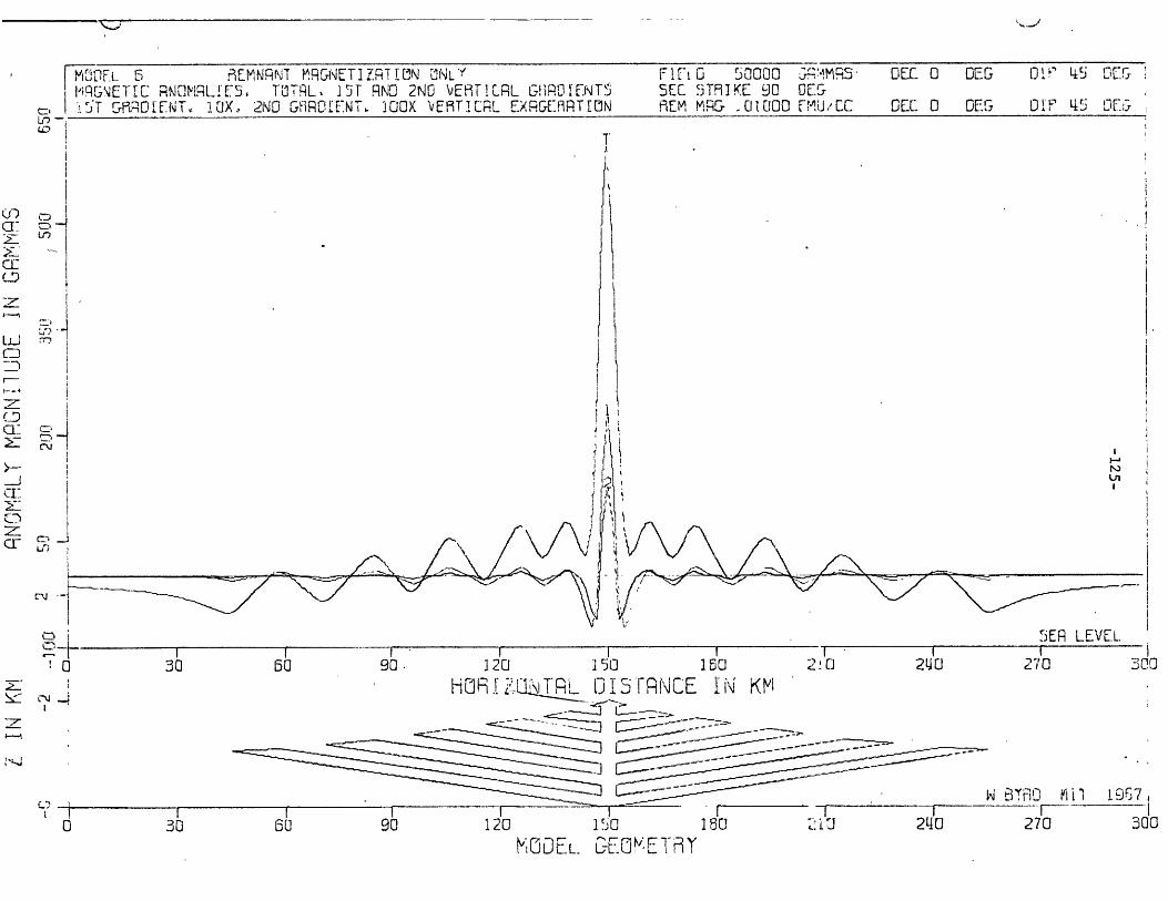
~iL~F.L ~ r! EMNRNT M9 NET1HRTEPI {NL'1'i~EiUI~L[7i~TU1TrlL. 15iT RNO 2NO VEiHTICLRL GHROIUANT
IZT RMTNT,- 1., 2ND GH1ROiEtJ 1 0OX VEt9TICL EXREERR[IN
IL 10 50000 JrlMMQ5.SEE 53T911 E 90 OcE&'-IIEM MIRI& .01000_Fllh1U/cc
orn E o0DEDEC 0 DEGO
DV" 4j5 LVY
-A--__________________________ ER LEVEL. IIII
50 90. 120 1530 150 21-0 2t10HOP i NT j 05 FPNOCE IN~ KM
......... . .......
MODEL &EO-ETLh
- f -IIS L"iu
W E ~3 T I tKiV i 1 1 67
2qO 270 300
Lo
rvD
270
120I

MODEL-. f3 FlMNRNT* rqCiET: 7Z.RTtl(.N ONL~e F!HT.0 50000MRGNETTCL RN!QMRLIT~i, ITTL, 1ST RNU 2N0 r1C1?IZ &,3R0lFNl5 SEC S3Y91KE 901!ST Gm0DL[TI !UX, 2NO4 GI . 2.OOX VE9TITJRL ._XRG3EHRTr0W -9rE-m mqr I!U-00
INJ
f I I50 90 120 ThU
hO~JIZ(]N!T~L GIoT~K~CE IN! ~ ~Kci -~
~-$Sc2-- -~ -
-- QQ~ -----
-~
2
A
0 .30 6 U 90 120 1Iw B T ID cl 11! I
210I
210 2'40 270
?30J
GRmmRs DEC 0 DEGY -~ L'4 L5 DOI-,,
cu~/rcC_ DEC 0 7 . 10 45 0E,
FR L E VEL.
i2 9 0 7 1II
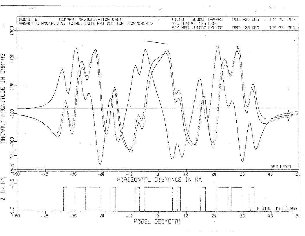
MODE *L. 9 9[MNRNT MPC NETI 7RT r ' N UN.'~~i~~~i~~Trc:~LI .~5L~~TTL iiz2OV~T.CRL ME'5t31ENJT5
. I-t0SEC Z'3T9!9 E MM ?R C"
50000
JllUi1000FC.C 5
DEC -25 D~--
1310 -75 iDEr
SEP LEVEL
Hl .. -/NJRL i N KM
W B 3fi 0 1MII
IV F-- C;"" F3Y ~ E T Fi Y
CD -
Ul)
,-
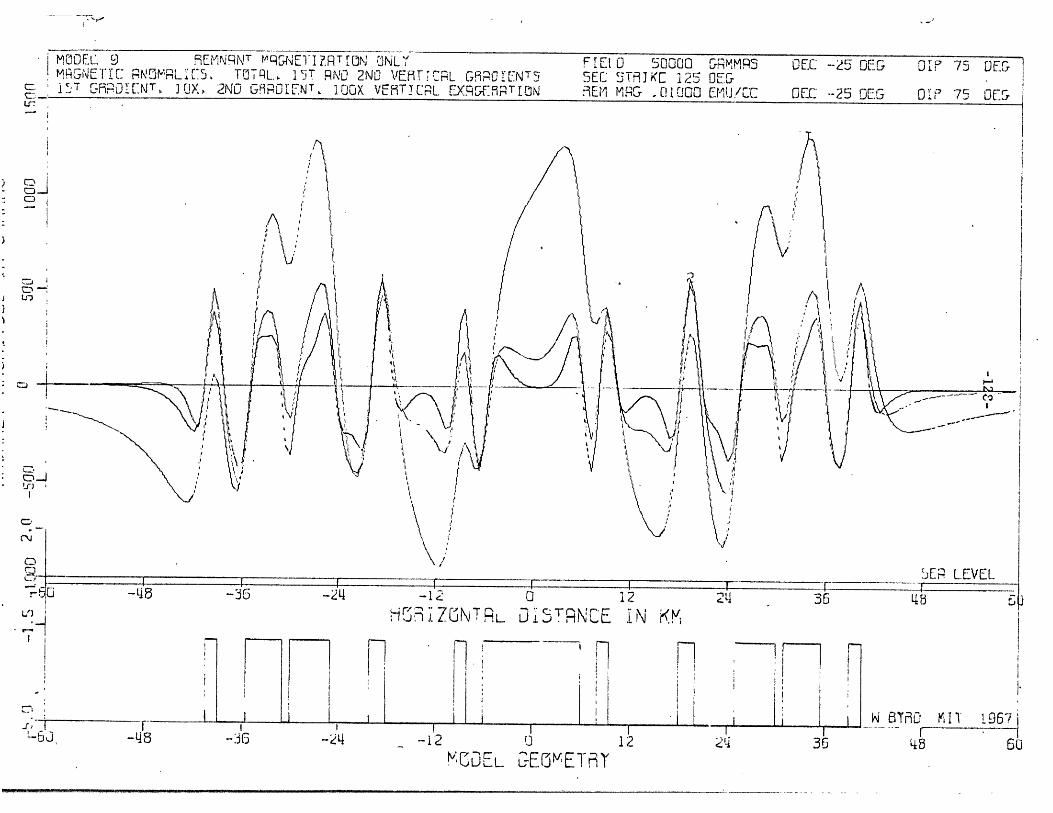
"L,,JVI rM,~f5, Tm-TqL,.~ 113T RND 2M0 VEMF0r-L GI9-0r"NTvic jT r7Fi2D-L- 1UX 2ND G JE. IOU V:FiT!C~L. ~9~Tj
CD.
FIl 50000 GrMM9551E C c5 T 91K C: 1 0 " -L,9 E t1 l MRG . Cl 1 00Etl f J,/CC
DEC-2 05E',
DC --25 fDEL--G
O 75 OEL5*
OW 75 0t73
'*ZUINTRL Di5TRNCE lN KmQ
! U LL &E[IET Y
48.

Mi~UEL9 INNT f9OrNETILJEATT.[lN UNL'~R~JTV NMRL~i~ TMTR . JiT UNICO 2tN4C 4Z-9,Z Pr!1N-T5
~ IJ ~i~rUN~IUX. 2N13 G IIPOY[7147 FUOK Rm2 C _- 9 T
F 1 EJ.D .50000 M, MP'cLC c--TjK 12': 0 E
1SD1ti tot 010 jru
o-'C __25 r-7
HOHJSZONTRL UI15TPKNCE IN KJI
5C LEVEL4b t]1
KiiDEt,- CEOMEITRY
tn
C,
L~L
-- .1f3CJ
-7 Ll c5 r-
7 75 0!o~
I ---- I J--k --
- r-
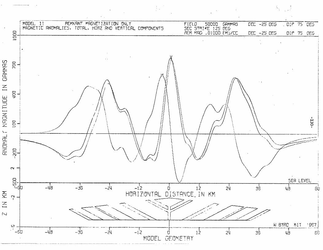
MODEL 1I REM'ThRNT MNETU7RTION ONLYMRGNETIC RNOMqLIES8I'ITLITRL, H-OflZ RNO 'EFRTICRL COMP'ONE1NTS
F IULO 50000 CrRMMRS5EC 5T~jKE 12"5 OEIG13Em mqO- ..Q100 EMU/cc
DEC -2c5 DEG
DEC -2~5 DEG-',,
CIF 75 DES
DIP' 7"., DOr
E3ER L.EVEL.
HOA91ZCNTRL )I .N C E. I'N K M
W BYRO tI T _9_
48 6uMODEL G'7EO V E TFY
-6o
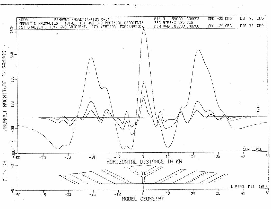
MODEL 1 REMNPNT MRCrEETIZR T ON UNLYMRGNETIC RNOMPLrES. TUTRL, 35T RNO 2NO VERT!CRL GRROIENT5IDr GRRDIENTI 10X. 2ND GRROENT 3OX VERTICRL EXRGERRT1rIN
L0
U-
FIELD 50000UUU LHRMMHSEC STRJKE 125 ODErREM M qG J01000 EMU/CC
L'LL -~ L.L7 uI (:3 ui:u-UCL -2L UtLL
DEC -25 DEG DIP 75 OEG
1 -2-36 -2
E LEVEL____ IF
I I I-12 0 12
HORIZONTRL DISFRNCE IN KM
-36 -24 -12 0
WT 6TFO MIT 19 C7
12 '2 36 4I 612 2 36 L
MODEL GEOMETRY
\/.
///Ir
M(I -
n doC14
.I--18
L6 I
-60I
-48
I
~ ii~-~ ---- -*iii~--- ------~--~---------~-~----- ---------------- ~-
- C C L IC CI I~- ~ T\~f,
--
I I I I
ULI tl UE."
rw
7---c/--
i
J-

REL 3.MI,\!RNT' ?IRWEIRTION UIL FWI LO 50000 I RMMQS*MHCNETI[ RN'0M9LIE5. TUjTqL, iJ7 9NC 2N'4O H09Z C41ROJE1N7 SEC 1'91 KE 125 OEG-I'JC-1mOlENT. IIIXP 2ND GFIR F.NT 100.XVE3TICIL EX.RG.ERRT~IO RE MR1G .0Q1000 EM/C
Ln
EC -25 DEG cir7
--EC 725 DEG DIP' 753 E&
ER LEVEL.
6HCPIZU'IL DISTRNCE IN KM
'N
MODEL, GIEOMETYIT
F, ~12 24 36
W BYR~D 'IlIT '.967--- 3I -2~4 -12
-133-
Biography
The author was born September 24, 1941 in Charlotte, North Carolina.
He attended North Carolina public schools and in 1959 he entered MIT. In
June 1963 he was graduated from MIT with a S.B. in Humanities and a minor
in Architecture.
He then joined the Woods Hole Oceanographic Institution and spent a
greater part of the following year aboard the Atlantis II as a member of the
International Indian Ocean Expedition. Here he became acquainted with
several oceans and seas and with the numerous ports which lie upon their
shores. In September 1964 he returned to NIT to continue his studies in
Oceanography. There he has remained except for brief excursions into the
world at/large.
He is an active member of Sigma Xi, the American Geophysics Union, and
the Marine Technology Society. He is a charter member and Resident
Oceanographer of the Green Street Oceanographic Institution.
Among his various non-professional interests are skiing, diving,
sailing, archaeology and photography. He considers essential good food,
wine and stimulating companionship. He is presently unmarried.