JPRS-JST-89-006 - I 16 MARCH 1989

FOREIGN ff \\W BROADCAST 11 ■ ' " INFORMATION

SERVICE

JPRS Report— 1 • ^pjpmfred lot poblie re'aAae;

Science & Technology

Japan

4TH INTELLIGENT ROBOTS SYMPOSIUM

VOLUME I

C9I2Z Un 'ai3IJ9NiadS ciy nwAoa iaod sszs

AUCIUHMUd Aia3n3a £01 SS3D0ad «MllU

SUN UP

19 III DTIC QUALITY INSPECTED 1

JPRS-JST-89-006 - I

16 MARCH 1989

SCIENCE & TECHNOLOGY

JAPAN

4th INTELLIGENT ROBOTS SYMPOSIUM VOLUME I

43064062 Tokyo 4TH INTELLIGENT ROBOTS SYMPOSIUM PAPERS in Japanese 13-14 Jun 88

[Selected articles from the 4th Intelligent Robots Symposium held 13-14 June 1988 in Tokyo]

CONTENTS

Underwater Surveillance Walking Robot Developed 1

Control of MELCRAB--Stair-Climbing Six-Legged Mobile Robot 14

Dynamic Walk Pattern of Four-Legged Robot 24

Kinematic Analysis of Four-Legged Walking Robots 36

Development of Adaptive-Locomotion-Type Four-Legged Robot 47

Research of Thrust-Powered Wall-Surface Walking Robot 55

Development of Wire-Suspended Robot 65

Development of Wheeled Wall Surface Walking Robot 74

Automatically Configuring Obstacle Avoidance Paths in Lattice-Point Space 84

Basic Research on Collision Avoidance Techniques for Mobile Robots.. 96

a

Collision Avoidance in Locomotion Robotic Systems 116

Search Capability of Locomotion Robot in Unknown Environment 126

Map Expression, Path Planning for Locomotion Robots 139

Intelligent Locomotion Robots for Autonomous Land Vehicle 149

Control Methods for Locomotion-Type Autonomous Robot 162

Tele-Vehicle I--Autonomous Remote Controlled Vehicle 173

Capture Operations Involving Orbiting Space Robot Manipulators 185

Development of Intelligent Robot for Nuclear Power Station 198

Underwater Surveillance Walking Robot Developed

43064062 Tokyo 4TH INTELLIGENT ROBOTS SYMPOSIUM PAPERS in Japanese 13/14 Jun 88 No 103 pp 21-26

[Article by Mineo Iwasaki, Junichi Akizono, Masashi Nemoto, and Osamu Asakura, Port and Harbor Research Institute]

[Text] 1. Foreword

Underwater surveys involved in port and harbor construction are conducted by divers. However, due to the special working conditions encountered underwater, such surveys are risky and their efficiency is low. The demand to replace divers with underwater surveillance robots has been heard due to the decreasing number of divers and the problems involving working conditions since port and harbor construction work increasingly involve deep waters.

To cope with the situation, the Transport Ministry's Port and Harbor Research Institute has developed the "Aquarobo," an axially symmetrical, six-legged insect-type program-controlled walking robot, as an underwater surveillance robot for port and harbor construction.

The Aquarobo walks on six axially symmetrical legs, each having three joints driven by a DC servomotor. Each joint is mechanically independent and all walking activities are controlled by a program.

Therefore, its walking is not limited. The robot is linked to control equipment aboard a mother ship with a cable.

The robot's main functions include conducting underwater observation with a video camera and measuring the seabed unevenness through walking. It is currently designed to walk on rubble mounds comprising the foundation of a caisson.

In FY 1984, the institute manufactured a robot for use in ground experiments which had legs half the length of those of the actual model, and conducted walking experiments after developing a flat surface walking program.1"2

Improvements were made on the experimental model in FY 1985 and, with the development of an uneven surface walking program, the robot successfully walked on a rubble mound installed on the ground in FY 1986.

We also experimentally manufactured a water-tight leg and a manipulator for an underwater video camera in FY 1985. With them, we developed the water- tight experiment model shown in Photo 1 [not reproduced] in FY 1986. Based on these achievements, we conducted successful underwater walking experiments using the water-tight model in the following fiscal year.3"4 We simultaneously conducted research to make the robot smaller and lighter, and designed and produced a lightweight water-tight leg with an improved joint structure in FY 1986 and a lightweight water-tight experimental model in FY 1987.

The practical model to be manufactured in the near future will be able to dive to a depth of 50 meters and will be used to inspect the flattened surface of rubble mounds, including measuring unevenness, monitor caisson installation work, and study and measure damage to marine structures at deep-water port construction sites, such as Kamaishi port where breakwaters are being built.

This paper outlines the research conducted since FY 1985.

2. Control Program

(1) Outline

The Aquarobo's walking activities have all been accomplished through software. Therefore, the robot's performance depends directly on the performance of the control program used.

The control program is hierarchized into a control system program and a walking algorithm program. As an interface for the walking algorithm program, the control system program contains so-called robot language. The robot language is designed for real-time linear interpolation and pulse synchronous output to permit the transmission of instructions for leg operations by orthogonal coordinate systems.

The control program is a dialogue-type program and the operator needs only to select an operation mode from the menu, then input the walking direction and distance for a straight walk and the angle of rotation for turning on a particular spot. The robot leg conditions are graphically displayed so that the operator can determine the attitude of the robot.

The languages used are BASIC and a machine language.

(2) Walking Patterns

The Aquarobo's standard walking pattern is generally a three-leg alternating walk. It can also walk in special patterns with different combinations of raised and ground-touching legs. The walking patterns are as follows:

1) Standard Pattern (three raised legs and three ground-touching legs)

Every other leg operates as a group of three, each group alternately. The walking speed is the highest.

2) Special Walking Pattern (two raised legs and four ground-touching legs)

Since at least four legs are always touching the ground, this pattern can handle a larger load and features higher stability than the standard pattern. The stability is similar to that of an eight-legged robot in a four-legged alternating walk mode.

3) Special Walking Pattern (one raised leg and five ground-touching legs)

At least five legs always touch the ground to support the maximum load and offer maximum stability. The traveling speed, however, is low.

4) Special Walking Pattern (one raised leg and four ground-touching legs)

In this pattern, the robot walks on only five legs. Equipped with a sensor, the remaining leg can be used as a hand, eliminating the need to add another manipulator. Since a leg also serves as a hand, we call this the octopus function.

5) Special Walking Pattern (one raised leg and three ground-touching legs)

The robot walks on only four legs. Even if one or two legs were to become inoperable during an underwater operation, the robot could continue to carry out the mission.

(3) Program Functions

To obtain the maximum performance of the articulation-type walking robot's characteristics, the control program has several functions.

1) Unevenness Measuring Function

The Aquarobo walks on an uneven surface, using a ground sensor attached to the end of each leg. This enables the operator to know the ground surface configuration from leg movements. Unevenness is measured by totaling the movements of the end of a leg from one position to the next position and obtaining the relative geographical relationships between the positions.

A major advantage offered by a walking robot is that it not only travels on legs, but also measures the unevenness of the ground surface it covers.

2) Leg Operation Range Extension Function

Walking generally requires the tip of the leg to move either horizontally or vertically on the sides of a rectangle in a linear manner--the leg must be raised, moved forward, lowered to the ground and then moved backward.

However, since the range of operation of the tip of an articulating-type leg is enclosed in a circle, as shown in Figure 1, an unlimited number of rectangles exist within that range.

Figure 1. Foot Operation Range

Initially, therefore, we selected one rectangle beforehand as the range of operation. However, selecting a rectangle poses a problem under this method. When the rectangle ABCD is selected, making the strides longer for a faster walking speed, the robot raises its legs lower and can cover only less uneven terrain. When the rectangle AEFG is selected, allowing the robot to raise its legs higher, the stride becomes shorter and the walking speed slower. Therefore, this method does not permit the effective use of the legs' range of operation.

We abandoned the idea of selecting a rectangle beforehand and opted to select the optimum rectangle for each step according to the terrain. This, however, involves complex calculations because the largest rectangle possible must be chosen within a three-dimensional space enclosed by a sphere since the legs' rectangles are not independent of each other and the legs touching the ground must operate in the same direction in synchronization. The weighing of the stride and the height to which the legs should be raised poses another problem.

Therefore, we developed another method under which the broken line in Figure 1 represents the lowest position of the legs. For example, when the legs are to be lowered along the straight line AE, the rectangle becomes AEFG and the stride, EF, will be short if the unevenness is great, with the legs not being permitted to touch the ground until they are lowered to the lowest position E, however, the rectangle will become ABCD when the legs touch the ground at B, making the stride longer. Therefore, the range of the legs' operation can be used efficiently in accordance with the position where the legs touch the ground.

The advantage of this method is that an appropriate setting of the curve minimizes the unusable range and, at the same time, weighs the stride and the height to which legs can be raised. The range of the legs' operation is

actually three-dimensional space, but virtually the largest rectangle for a leg's next move from its current position can be calculated from the shape characteristics of the range of leg operation and restricting conditions.

Since the method allows the leg operation range to be changed according to the terrain, actually providing a range-extending effect, we refer to it as the leg operation range extending function.

3) Ground Retouching Function

If a leg cannot touch the ground during walking, even when it is lowered completely, the robot judges it is impossible to touch the ground at that point and lowers the leg to another point. When the robot fails to touch the ground with a leg after several trials at different points, "ground touching impossible" will be displayed on the screen and the display will return to the menu.

4) Body Inclination Changing Function

Usually, a walking robot walks, maintaining its body level. It is necessary to return the body to a level position when it is inclined due to the slipping of a leg or the collapse of the ground.

The body inclination changing function changes the inclination of the body. In our program, the center of gravity is regarded as the center of motion, so that no shift in the center of gravity of the robot body will occur.

It is important to note that, in changing the attitude of a walking robot, relative positional relationships of the ground-touching legs must not be changed. Calculation becomes complex, especially when the robot is walking on an uneven surface.

Initially we calculated the XY-direction inclination correcting angles separately and totaled them as a simple calculation method, but the end of the legs slipped, indicating that errors could not be ignored.

The direction of the body's largest inclination generally crosses the body's XY axis if not at right angles when projected onto a horizontal surface. Errors were caused because the inclination sensors were attached in the XY- axis direction of the body and X- and Y-direction inclination correcting angles were not independent of each other.

Therefore, we developed a formula to analytically determine the direction and size of the body's largest inclination from information obtained by the sensors, and solved the problem by controlling the legs through coordinate transformation in the direction of the largest inclination by using the precise answer obtained from the formula. As a result, the legs stopped slipping.

5) Inclined Walking Function

The inclined walking function permits the robot not only to maintain the body level, but also to keep the body inclined at a desired angle while walking. The robot sometimes cannot walk on a slope, maintaining the body level, because the legs hit the ground. In such a case, the robot can walk by inclining the body in the direction of the ground inclination.

However, such a move causes a shift in the center of gravity to occur in robots controlled by a coordinate system fixed to the body, and it is necessary to avoid this shift by employing the limited movable range walking mode, or the inverted trapezoid walking mode for four-legged robots.5

This problem can be solved by setting the control coordinate system in the perpendicular and horizontal directions irrespective of the body's inclination. This solution involves difficulties in controlling walking robots controlled by a rectangular coordinate system fixed to the body because coordinate transformation is required. However, the program- controlled Aquarobo requires coordinate transformation and little change in control complexity occurs.

6) Walking Parameter Estimating Function

Parameters for walking, such as the stride, the height the legs should be raised, the height of the body and the inclination of the body, are generally set by the operator beforehand and remain unchanged during a walk. However, when the robot travels on a changing terrain, e.g., from a slope to level ground, it can walk efficiently without making useless leg movements if the parameters are changed in accordance with the ground conditions.

The walking parameter estimating function determines the extent of unevenness from the legs' positional relationships by using the unevenness measuring function and automatically selects the optimum walking parameter values, employing the inference algorithm. This function includes a decision to determine whether the leg separation range extension function and the inclined walking function should be employed.

3. Improvements of Land Experiment Model and Walking Experiments

We improved the land experiment model manufactured in FY 1984, including a change in the leg structure and the installation of various sensors, enabling it to walk on a rubble mound-like uneven surface in 1985.

Table 1 shows the specifications of the land experiment model after the improvements.

(1) Walking Experiment on Rubble Mound

We conducted walking experiments on land on a roughly and fully leveled rubble mound to study the walking performance of the land experiment model and the adequacy of the control program.

6

Table 1. Specifications of Land Experiment Model (Improved)

Robot

Type

Driving system

Control

Unevenness covered

Major material

Weights

Dimensions:

Number of joints

Sensors used

Dimensions

Front panel

Computer

Others

Axial-symmetrical six-leg walking insect type (with three joints for each leg)

DC servomotor semidirect drive

Program controlled by personal computer

±17.5 cm

Corrosion-proof aluminum

280 kgf

Body: hexagonal column with each facet measuring 16 (H) x 25 x 25 m Leg length: Body side: 25 cm

Foot side: 50, 55,60 cm Foot diameter: 16 cm, ankle movable angle: ±45

degrees (all around)

18 for legs, 1 for obstacle sensor supporting arm, 19 total

6 tactile sensors (leg end) 6 eight-part tactile sensors n sole (foot) 6 foot-side tactile sensors (foot) 2 inclination sensors, 1 azimuth sensor (body top) 1 obstacle sensor (tip of arm)

Control equipment

1,710 x 2,050 x 810 mm

Terminals and displays for joint voltage, inclination sensor, azimuth sensor, and obstacle sensor readouts

16-bit personal computer (CPU: i8086)

Joint torque sensors (for the second joints) and encoder counters

The rubble mound used for the experiments consisted of a level section, 3 m wide and 6 m long, and a slope with a 25-percent inclination. The mound was manufactured by divers actually engaged in leveling work and used real rubble. The leveling precision was ±5 cm for full leveling, the same as

that of actual rubble mounds, and ±15 cm for rough leveling, half that of actual mounds since the leg length of the experimental model was half that of the practical model's legs.

Based on the results of preliminary experiments, we manufactured robot feet of the optimum shape and size for rubble mound walking and replaced the original feet with the new ones. They are 25 cm in diameter and the base is flat and rubber-coated.

The robot proved capable of walking problem-free on a roughly leveled surface. Walking speeds depend on the stride and the height to which the legs are raised. In the experiments, the maximum speed was about 1.7m per minute, with the joint rotating speed set at a quarter of the maximum operating speed. The walking speed increased as the joint rotating speed was raised, but we did not increase the speed any further in the experiments due to inertial mass problems and the reliability of the ground touching sensors and also because the robot cannot walk as fast in water as on land due to fluid resistance.

The inclined walking and walking parameter estimating functions were added to the control program based on information obtained from the experiments. The inclined walking function enabled the robot to walk on a 25-percent grade, which had previously been difficult. Photo 2 [not reproduced] shows the robot covering the grade. The walking parameter estimating function slashed the time required for ascending a slope to about one-third the previous time.

The experiments demonstrated that the Aquaboro can walk autonomously, selecting optimum walking parameters through program control, on ground with unknown terrain. Particularly notable is that it was able to climb up and down a slope with an uneven surface on its own, and we believe we have cleared one of the hurdles for the development of a practical use walking robot.

(2) Durability

The land experiment model was displayed at "Tohoku's Future Exhibition" held in Sendai, Miyagi Prefecture, from July to September 1987, where it demonstrated its walk, using various walking patterns, on a flat surface and a simulated rubble mound.

Although some minor problems occurred the robot was inoperable for only 2 days, in September, of the 73-day run of the exhibition. The problem was caused by a cable connecting the body and the legs and had nothing to do with the robot's main mechanism.

We think the land experiment model proved sufficiently durable in view of the fact that although brand-new walking robots are usually displayed at science exhibitions, our robot had already been used in experiments for 2 and 1/2 years.

4. Manufacture of Waterproof Experimental Model and Underwater Experiments

We experimentally-manufactured one waterproof leg in FY 1985, and based on the results of experiments with it, we manufactured a waterproof experimental model in FY 1986. Signal transmission is done by optics, and the robot and control equipment are connected by an optoelectronic composite optical fiber cable. The robot has photoelectric converters within the body and the control equipment. Multiplexing is used for signal transmission to reduce the number of optical fibers used.

Table 2 shows the specifications of the waterproof experimental model.

(1) Robot

The leg length of the robot is double that of the land experiment model. The shape and major dimensions are shown in Figure 3, while Photograph 3 [not reproduced] shows both models for purposes of comparison.

5th leg 6th leg

4th leg

Underwater posi- tion finder (mas ter station)

2d leg Underwater video earner

Manipulator

Foot

Tactile sensor

Figure 3. Shape and Major Dimensions of Waterproof Experimental Model

On the top of the body, we installed the manipulator for an underwater video camera manufactured in FY 1985. The manipulator has 3 degrees of freedom and weighs about 70 kg, excluding the camera, on land. In order to widen the vision of the video camera, we employed the joint direct drive system, the same as that for the robot's legs, without using the link system that has a restricted range of motion and is difficult to make waterproof.

Table 2. Specifications of Waterproof Experimental Model

Robot

Type

Driving system

Control

Unevenness covered

Waterproof

Major material

Weight

Dimensions

Number of joints

Sensors used

Axial-symmetrical 6-leg walking insect type (with 3 joints for each leg)

DC servomotor semidirect drive

Program control by personal computer

±35 cm

To depth of 50 m

Corrosion-proof aluminum

689 kgf (on land), 320 kgf (in water)

Body: 77-cm high cylinder with 50-cm diameter Leg length: Body side 50 cm, foot side 100 cm Foot diameter: 25 cm Ankle movable angle: ±45 degrees (all around)

18 for legs and 3 for manipulator, 21 total

6 tactile sensors (leg end) 2 inclination sensors, 1 azimuth sensor (inside body) 1 depth sensor (lower body)

Control equipment

Dimensions and weight 1,230 x 1,600 x 800 mm, 250 kgf

Front panel

Computer

Optoelectric conver- sion equipment

Terminals and displays for joint voltage, inclina- tion sensor, azimuth sensor, and depth sensor readouts

16-bit personal computer (CPU: i80286)

1 for TV picture signals, 5 for encoder signals and 1 for sensor signals

Composite cable

Dimensions Unit weight Specific gravity Allowable tension

42 mm (diameter) x 100 m (length) 1,660 g/m (on land), 370 g/m (in water) About 1.28 1,500 kg

10

The actuators for the first and second joints from the base of the manipulator are placed close to the base in order to increase the load that can be handled. The first joint is doughnut-shaped, with cables going through the central hole so that they will not interfere with the manipulator's movement while it is turning.

Waterproof magnetic proximity switches were adopted for ground-touching sensors so that they could operate at constant force irrespective of the depth.

As for the robot feet, we used the same shape and measurements as those used by the land experiment model for rubble mound walking experiments. The underwater model is not equipped with eight-part touch sensors for the foot bottom and touch sensors for the side section since such sensors cannot be used under water.

(2) Control Equipment

We made the control equipment compact for easy loading on the mother ship. The adoption of a small servo driver and an overall review of the configuration shrank the control equipment size to about one-third that of the land model's in terms of volume, despite the fact that it has a built- in photoelectric converter and interface box. Photograph 4 [not reproduced] compares the control equipment for the land and underwater models.

(3) Tank Experiments

We conducted underwater walking experiments on the waterproof experiment model in a tank, as shown in Photograph 5 [not reproduced].

In the walking experiments in the tank, we studied a decrease in the walking speed due to fluid resistance and an increase in required joint torque on a flat surface, the maximum walking speed in the tank has reached about 1.4 m per minute so far.

In underwater walking, the walking speed is limited by the robot's inertial mass and fluid resistance. The feet slipped when the walking speed during a straight walk was increased, although no problems occurred in pivoting on the spot. This indicates that inertial mass affects the robot's walk more than fluid resistance does. For the time being, we plan to cope with the problem by optimizing the time constant of the servodriver. In order to increase the walking speed, we think it is necessary to make the robot smaller and lighter.

(5) Undersea Experiments

Using the waterproof experimental model, we carried out undersea experiments in december 1987 in the Yasuura area of Yokosuka Port. Photograph 6 [not reproduced] shows the robot during an undersea experiment.

Walking experiments were conducted on an actual rubble mound at a depth of 5.5 m to confirm the robot's walking performance under actual conditions.

11

The robot carried an underwater video camera with an ultrasonic range finder and an underwater position finder to evaluate the entire system.

Equipped with the ultrasonic range finder and an optical system designed specifically for underwater use, the video camera can measure the distance to a subject. Horizontal and vertical scales are superimposed on the screen, and it can measure the subject's size with a cursor, with its calculations based on the picture angle.

The underwater position finder is an LBL-system ultrasonic transponder. Consisting of one main station and three substations, it can measure the robot's three-dimensional position. It uses linear frequency modulated (FM) signals, seldom used in the audio field, as the carrier, and adopts the pulse compression method for frequency modulation to reduce multiple reflection. As a result, it offers the high precision of ±10 cm for a distance of 300 m.

For the undersea experiments, we manufactured a reel that can take up the optical fiber cable, without twisting it, as a support system.

We conducted 10 walking experiments at a speed of one-eighth of the maximum walking speed, and generally obtained good results for the walking and unevenness measuring characteristics. Pictures sent from the video camera attached to the manipulator did not shake during the robot's walk, attesting to the fact that the waterproof experimental model could maintain the levelness of the body while walking. The robot sometimes caught its feet between rubbles. Therefore, the foot shape needs to be improved.

We also checked the performance of the video camera equipped with the ultrasonic range finder and the underwater position finder, and they proved to provide the required performance.

Based on the results of the underwater walking experiments, we are improving the waterproof experimental model for practical use. We manufactured floats to help reduce the impact on the robot when it is dropped into water and hits the sea bottom, and replaced the robot's magnetic azimuth finder with a gyroscope-type one. We also plan to boost the output of the joint actuators and improve the foot shape.

5. Conclusion

Walking robot research has progressed from the walking experiment stage to that for practical use with specific objectives.1 However, the walking robots manufactured so far are actually experimental models, and no robot has been made yet for practical use.

We believe the Aquarobo, which can walk on a slope with an uneven surface and has actually walked in a natural environment under the sea, most closely approaches a commercial-use model.

The development of the Aquarobo, which began in FY 1984, has entered its final phase, and the improved waterproof experimental model is scheduled to

12

undergo practical use tests in Kamaishi Port at a depth of more than 30 m during FY 1988. We hope to solve the problems that remain before it can be used in actual harbor work through tests and further improvements.

References

1. Junichi Akizono, et al., "Development of Walking Underwater Survey Robot," Collection of papers prepared for the Third Intelligent Walking Robot Symposium, Japan Robotics Society, June 1986, pp 31-36.

2. Junichi Akizono, "Current Status of Underwater Survey Robot Development and Its Problems," Text prepared for Fifth Technical Lecture Meeting on Construction Robots, Civil Engineering Society, November 1986, pp 13-25.

3. Mineo Iwasaki, et al., "Development on Aquatic Walking Robot for Underwater Inspection," Report of the Port and Harbor Research Institute, Vol 26 No 5, December 1987, pp 393-422.

4. Junichi Akizono, "Walking Underwater Survey Robot 'Aquarobo,'" SAGYOSEN, Japan Working Ship Association, No 175, January 1988, pp 10-17

5. "Study of Four-Legged Walking Machines' Intelligent Determination of Walking Modes and Basic Considerations on 10 Slope Walking Modes," Collection of papers prepared for the Fourth Scientific Lecture Meeting of the Japan Robotics Society, 1986, pp 383-386.

13

Control of MELCRAB--Stair-Climbing Six-Legged Mobile Robot

43064062 Tokyo 4TH INTELLIGENT ROBOTS SYMPOSIUM PAPERS in Japanese 13/14 Jun 88 No 104 pp 27-32

[Article by Noriho Koyauchi and Adachi Hirotsuke, Mechanical Engineering Institute; and Aji Nakano, Tohoku University]

[Text] 1. Introduction

Many studies of legged mobile robots have focused on the complex control of degrees of freedom through multijoint leg structures.1 However, during a quiet walk with three or more legs always touching the ground, the legs form a mechanically closed loop via the ground surface, causing mechanical interference among them. Just as in controlling multiple manipulators or fingers, spatial interference, that is, a collision, of the legs must be avoided for a walking robot. To continue a smooth walk, it is necessary to select a walking mode that will ensure that the supporting polygon2 formed by the supporting legs continuously contains the center of gravity. The redundancy in the degree of freedom is designed to cope with varied walking environments, but the load of the control program tends to become larger during basic walking operations than when dealing with terrain conditions. An energy loss also tends to be caused by dynamic interference and relationships between the leg mechanism and dead load support counterforce. The Mechanical Engineering Laboratory has been conducting research and development of the MELCRAB-13 (Figure 1 [not reproduced]), a six-legged mobile robot, and the MELCRAB-2* (Figure 2 [not reproduced]) to solve these problems involving the basic walking movements of machines and to increase the control of terrain adaptation, particularly the descending and ascending of stairs. This paper discusses the basic configuration of such control.

MDA and Pseudolinear Mechanis m

It is known from analyses of the walking patterns of insects that the alternate three-point grounding method provides the fastest walking speed in hexapod walking machines.5 The gravitationally decoupled actuator (GDA) has been proposed to curtail the energy loss which occurs during walking by separating the legs' degrees of freedom in gravitational and horizontal directions.6

14

We adopted the motion decoupled actuating (MDA) method under which the horizontal propelling of the mobile unit and the adaptation to a rough ground surface are accomplished by mutually noninterfering different degrees of freedoms.7 Under this method, the mobile unit's motion is divided into propelling motion and terrain adapting motion, and totally different degrees of freedom constitute and drive each category. The leg conditions during walking are generally classified into the standing-leg and idle-leg phases. In the standing-leg phase, the ground-touching point does not change until the next step and a mechanically closed loop is formed among the robot body, leg and ground, as explained earlier, requiring complex control. The relative motion of the ground and body, however, can be reduced to one- dimensional motion. By contrast, in the idle-leg phase the leg must touch the ground in accordance with the terrain configuration, but it will not interfere dynamically with other legs due to the open link. A cyclic motion generally dominates the walking motion, as shown by animal locomotion, and in many cases terrain-adapting action is taken as a fine adjustment measure when an idle leg touches the ground. Therefore, no mechanical interference among the legs will occur when a cyclic return motion of the standing-leg phase trajectory and the idle leg is achieved by mechanically coupling the legs. It is also thought possible that the motor's motion energy loss can be lessened by fixing the propelling motion to the mechanically drawn trajectory.

.^-i---

Figure 3. Approximately Straight Line Mechanism

The approximately straight line mechanism8,9 shown in Figure 3 was adopted, based on these ideas, for the robot body propelling motion. It is called Chebyshev's approximately straight line mechanism and generates a locus quite suitable for walking, as shown in the figure. This approximately straight line section is used for the horizontal direction of the GDA, while the rack-and-pinion direct-drive extension/retraction mechanism, shown in Figure 4, is employed for the perpendicular direction.

3. Control Hardware Configuration and Hierarchical System

Figures 5 and 6 show the control system configurations of the experimentally manufactured MELCRAB-1 and MELCRAB-2. The MELCRAB-1 has potentiometers, tachogenerators, rotary encoders, and attitude sensors as internal sensors,

15

Figure 4. Mechanism for Leg-Extension or Retraction

Figure 5. MELCRAB-1 Control System

and analog touch sensors at leg ends and ground touching sensors on the soles as external sensors. In the MELCRAB-2, the analog sensors were replaced with optical digital sensors and infrared proximity sensors were added to detect objects before being hit by the legs. The first thing we wanted to avoid was the attitude giving way when the body goes up and down due to the extension and retraction of the legs. Therefore, both the servo driver unit in Figure 5 and motor driver in Figure 6 have analog velocity feedback circuitry with tachogenerator voltage feedback. This is the hardware that constitutes the lowest level of the hierarchical control system.

Walking robots generally have a hierarchical control system because they have many independent degrees of freedom.10-11 Different types of high-level control systems, including motion commands from the operator, interfaces and terrain surveillance using machine vision can exist. Since external sensors

16

Figure 6. MELCRAB-2 Control System

are used only as leg sensors in the experimentally manufactured models due to sensor installation conditions, the hierarchical structure of the control system will be similar to that shown in Figure 7. A velocity feedback servo mechanism, made up of analog circuits, which is most close to hardware, constitutes Level 0. Level 1 involves the position control of the body propelling and leg extension/retraction motions, providing the software servo is based on values given by rotary encoders or potentiometers.

level.3

level.2

level.1

Terrain adaptin« control tactlscs

Input of tactile sensor siintls and adaptint

aotion control

Pos 11Ion control of body-prop«!I Ini and

let extend i nt

level.0 Velocity control of body-propel Ii nt and

let extend int

Figure 7. Hierarchical Control System

The output is the command voltage of the Level 0 analog circuits. The input of tactile sensor signals and adapting motion control, such as the leg grounding and stoppage accomplished by sensor signals and position control, are on Level 2 and constitute a factor of Level 3. In the control program, Levels 1 and 2 together form a subprogram. On Level 3, the top level, terrain adapting control tactics, which will be explained later, are found. Currently, the operator's motion commands are the sole input to this level and its parameter is the number of steps.

17

4. Leg Position and Speed Control

Due to the adoption of the approximately straight line mechanism and the MDA, the leg position and velocity control on the lowest level require no complex trajectory generation. We adopted the semi-software servo loop, consisting of analog velocity control and digital position control, shown in Figure 8. the position control for an approximately linear motion are noncontinuous values since the sensor input is executed by rotary encoders. Therefore, we decided to carry out control through a transformation into relative coordinates which contain the target position as a positive value, with the initial position set as the origin for each step. Under this position and velocity control, the target position and maximum velocity while traveling to that point are given as command values. Continuous control of the trajectory is not required due to the velocity feedback servo mechanism of the analog section, and PTP control suffices.

Figure 8. Semi-Software Servo Loop for Position and Velocity Control

5. Terrain Adapting Control Tactics

5.1 Obstacle Avoidance Control12

One of the ways to cover rough terrain by using tactile sensors is simple obstacle avoidance. The tactile sensor on each foot is monitored constantly and the body propelling motion is suspended when an obstacle is detected, with obstacle avoidance actions taken repeatedly by retracting idle legs or extending supporting legs until the sensors no longer detect the obstacle. Upon completion of the avoidance operation, the body propelling motion resumes. The obstacle avoidance control is applicable not only to stairs, but also rough terrain surfaces. Figure 9 shows the foot trajectory in obstacle avoidance control during stair climbing.

5.2 Stair Dimension Learning Control13

When the surface to be covered is a combination of a flat area and stairs, it is possible to change the foot trajectory by learning stair dimensions from tactile sensor information, making use of the regularity of the stairs. The robot walks on a flat surface with the body propelling motion using the approximately straight line mechanism and, when it detects an obstacle, it assumes that the obstacle is a staircase. With the initial tactile information, the robot learns the position X0 of the first step of the stairs, and with the next batch of tactile information it learns the position of the second step and, at the same time, calculates the depth d of the step. In six-leg grounding, in which idle legs become standing legs,

18

Foot trijectory

Figure 9. Foot Trajectory in Obstacle Avoidance Control

the step height h can be calculated. Since it is possible to use X0, d, and h to predict the edge of the stair step the robot will encounter in its next step, the robot can climb the stairs without stumbling by simultaneously carrying out the body propelling motion and terrain adapting motion (leg extension/retraction) by setting the target value at a point slightly higher than the edge. In the obstacle avoidance control explained in 5.1, the body propelling motion ceases frequently because the six legs touch the stairs with every step. The more frequent the stop-avoidance-reacceleration procedure is utilized, the slower the traveling speed of the robot becomes. In stair dimension learning control, however, the robot stops only at the first stair step. After calculating the stair dimensions, the robot can climb the stairs at a speed close to that of a flat surface walk because no sensor touches the stairs except when the standing legs are changed. Figure 10 shows the foot trajectory in stair dimension learning control.

Foot trajectory

Figure 10. Foot Trajectory in Stair Dimension Learning Control

6. Synchronization Control of Two Body-Propelling Degrees of Freedom"

Landing points cannot be changed in the MELCRAB-1 because the approximately straight line mechanism of all six legs is mechanically linked. As for the MELCRAB-2, we made a landing point change possible when two sets of three legs exchange roles in the alternate three-point landing pattern by driving the two groups of legs with separate motors. The MELCRAB-2 requires a control program for idle and supporting leg synchronization, which is not needed for the MELCRAB-1. Figure 11 shows the servo mechanism of the control. In the figure, 6n and 0s are phase angles of the input axis of the approximately straight line mechanism that carries out the synchronization, and represent the master and slave, respectively. Driving must be done with the slave angle targeted at a value 180 degrees phase-different from the master angle. Input parameters are the master angle's target value 6m and its maximum speed 9m. The master is PTP-controlled from its original

19

8Md r^kej--' V

-Y&t&^&f*

—tsHi3~4__J~*?H&©*<T( ̂J*

Figure 11. Block Diagram of Synchronization Control of Two Body-Propelling Degrees of Freedom

position as opposed to the target value, while continuous value control is used for the slave, with target values set at the master's present position and maximum speed. Limiter 2 in Figure 11 is provided to prevent giving commands for excessive speeds, averting having the slave being driven in the opposite direction from the master. From the viewpoint of stabilization during walking, we concluded that the supporting leg group should serve as the master and the idle leg group as the slave. Figure 12 shows the results of a synchronization experiment involving two body-propelling degrees of freedom. Figure 12(a) shows the input angle of the approximately straight line mechanism, with the broken line representing 0M and the solid line 0s. The chain line represents the difference between the slave's target value and the present value, with CMS ■ (0M + n - 0s). Figures 12(b) and (c) show the command voltage output value from the digital/analog (D/A) converter to the analog velocity feedback circuit and the tachogenerator# voltage, respectively, with the broken line representing angle velocity 0M and the solid line 0s. The experiment was conducted using the initial values of 6m - 3/4 n and 6so - 3/2 7r and the stop target values of 0Md - 3/2 jr and 0sd - 7r/2. It is clear from the figures that the idle legs catch up with the standing legs through quick acceleration. When the slave is trying to catch up with the master, the command voltage is limited toJsum, the upper ceiling shown in Figure 11. In the Figure 12 experiment, 6sum « 2 6m.

As shown in Figure 12(b), excessive acceleration is avoided by increasing the command speed for alternating current from the original position to the maximum speed almost proportionally, in addition to proportional control near the target position. Since no interrupt control using a lock is employed in the MELCRAB-2's control system, the time-proportional alternating current generally used is not possible. instead we used the value obtained by multiplying the travel distance from the initial position by a gain and adding a constant as the command speed.

7. Conclusion

Since the MELCRAB-1 and MELCRAB-2 hexapod mobile robots use the approximately straight line mechanism and the MDA, they can walk without requiring complicated calculations for trajectory and gait plans for each

20

a b

a 1

0

-—•«—._^_

^^^

Figure 12.

i

a

I nie (•■•)

(a)

_\»-A— r (b)

r

I 2 TIIC (MI)

(c)

Synchronization Experiment of Two Body- Propelling Degrees of Freedom

leg. This paper discussed the basic structure of the robots' control, the stairs/rough terrain walking algorithm using tactile sensors and synchronization control for the MELCRAB-2.

We are now studying how to apply learning control using tactile sensors, used for stair climbing, to walking on general rough terrain areas.

21

References

1. INTERNATIONAL JOURNAL OF ROBOTICS RESEARCH, Special issue on legged locomotion, Vol 3 No 2, Summer, 1984.

2. A.A. Frank, "Automatic Control Systems for Legged Locomotion Machines," USCEE REPORT, 1968.

3. Eiji Nakano, Noriho Osanai, Makoto Kaneko, Hironori Adachi, Taketoshi Nozaki, Kiichi Ikeda, Minoru Abe, and Hidehiko Takano, "Development of Stair-Climbing Fixed-Gait 6-Legged Mobile Robot (First Report)-- Basic Design and Manufacture of Model," Collection of papers prepared for delivery at First Lecture Meeting of Japan Robotics Society, 1983.

4. Noriho Osanai, Hironori Adachi, and Eiji Nakano, "Free-Standing 6- Legged Mobile Robot MELCRAB-2--Semi-Fixed Gaits by Electrical Linking," 3d Intelligent Mobile Robot Symposium, 1986.

5. James Gray, "Animal Location," William Clowes & Sons, 1968.

6. Shigeo Hirose, Tomoyuki Masui, Hidekazu Kikuchi, Yasushi Fukuda, and Yoji Umetani, "Structure and Basic Characteristics of 4-Legged Walking Machine TITAN III," 2d Intelligent Mobile Robot Symposium, 13/19 1984.

7. M. Kaneko, M. Abe, and N. Tanie, "A Hexapod Walking Machine with Decoupled Freedoms," IEEE J. ROBOTICS AND AUTOMATION, Vol RA-1 No 4 1985.

8. Minoru Abe, Makoto Kaneko, Kazuo Tanie, and Shoichiro Nishizawa, "Study of 6-Legged Walking Machine Using Approximately Straight Line Mechanism," 2d Intelligent Mobile Robot Symposium, 27/32, 1984.

9. Minoru Abe, Makoto Kaneko, and Shoichiro Nishizawa, "Basic Study of 6-Legged Walking Machine Using Approximately Straight Line Mechanism, " Collection of Theses of Measuring and Atomic Control Society, Vol 21 No 6, 1985.

10. Shigeo Hirose and Yoji Umetani, "Structure and Experiments of Basic Motion Control System of 4-Legged Walking Machine," Ibid., Vol 16 No 5, 1980.

11. Shigeo Hirose, Yasushi Fukuda, and Hidekazu Kikuchi, "Control System for 4-Legged Walking Machine," JAPAN ROBOTICS SOCIETY MAGAZINE Vol 3 No 4, 1985.

12. Noriho Osanai, Eiji Nakano, Hironori Adachi, Makoto Kaneko, and Minoru Abe, "Development of Stair-Climbing Fixed-Gait 6-Legged Mobile Robot (Second Report)," Collection of papers prepared for delivery at Second Japan Robotics Society Lecture Meeting, 1984.

22

13. Hironori Adachi, Noriho Osanai, and Eiji Nakano, "Stair-Climbing Pattern of Fixed-Gait 6-Legged Mobile Robot (Second Report)," Collection of papers prepared for delivery at Third Lecture Meeting of Japan Robotics Society, 1985.

14. Noriho Osanai, Hironori Adachi, and Eiji Nakano, "Development of Stair-Climbing Fixed-Gait 6-Legged Mobile Robot (Fourth Report)--Semi- Fixed Gait Synchronization Control of MELCRAB-2," Collection of papers prepared for delivery at Fifth Lecture Meeting of Japan Robotics Society, 1987.

23

Dynamic Walk Pattern of Four-Legged Robot

43064062 Tokyo 4TH INTELLIGENT ROBOTS SYMPOSIUM PAPERS in Japanese 13/14 Jun 88 No 105 pp 33-38

[Article by S. Hirose and T. Takagi, Tokyo Institute of Technology; and T. Furutani, Yokogawa Electric Works, Ltd.: "Research on Dynamic Walk Pattern of a Four-Legged Walking Robot"]

[Text] 1. Introduction

Walking can roughly be divided into static and dynamic aspects from the standpoint of stability retaining. In the former, the center of gravity of a walking body is always positioned inside a polygon formed of the supporting legs and their soles, assuring static stability, while in the latter, on the other hand, it is sometimes found outside the polygon, requiring dynamic position-retaining control.

The authors have been engaged in the systematic study of the static walk of a four-legged machine. However, the capabilities of low-speed static walk alone are not sufficient to enable such a four-legged walking machine to be used as practical, universal moving platform, although it is highly stable. Namely, it is indispensable that it also perform dynamic walk that would ensure high-speed movement, even though swing would occur.

Several pioneer research projects have already been carried out involving the dynamic walk of walking machines. The main subject of most of them has involved the retention of their dynamic position. The authors, however, believe that it should not be extremely difficult for four-legged walking machines to retain their dynamic position, and that they should be able to perform dynamic walking without requiring any large-scale dynamic control. If dynamic walk could be performed easily, the machine's computer capability could be used to attain a high ground adaptability, significantly improving its functions. This paper will discuss the minimum problems to be solved to attain dynamic walk from this viewpoint. The appropriateness of this concept will be verified experimentally.

24

2. Basic Setting

2.1 Symbols To Be Used and Their Significance

The following are the symbols to be used here and their significance:

a: acceleration upon starting and completing resetting phase ß: duty factor-ratio of supporting phase time to leg unit cycle time T: unit cycle time of reference gait Vr: resetting speed of legs (relative to center of gravity) ^rmax: maximum mechanical value of Vr VG: gravity center shift speed XQ, x , z0, z*: movement range of legs (Figure 1) A : length of stride (A*max - x*) hu: ascending stride

III 4

Figure 1. Subject Four-Legged Walking Machine

2.2 Subject Walking machine and Its Gait

Figure 1 shows a subject walking machine model, as well as its leg movement range and coordinate system. Studied here will be dynamic walk to achieve normal straight advance on flat ground. Therefore, its y-directional freedom is ignored.

Gait (pattern of leg movement): static walk is based on a crawl gait and dynamic walk is based on a trot gait with 0.75 > ß > 0.5.

3. Acceleration and Deceleration Taken Into Account in Determining Leg Trajectory

For high-fidelity reproduction of walking movements, the leg trajectory must meet certain gait parameters, such as duty ratio, movement speed, leg resetting speed, etc.

When the leg's acceleration and deceleration time is not taken into account, the center of gravity VG of a walking machine and the resetting speed Vr of its legs have the simple relationship represented by:

25

1 -ß V, o V,

ß

(1)

This is derived from the fact that areas Sx' and S2' become equal in such a leg speed plan, as shown in Figure 2(a). The leg swing trajectory for static walk has been determined in the combination with its relationship to z (vertical)-direction movements.1 When the swing speed of the legs is increased, however, the target leg trajectory value of equation (1) is not practicable since their acceleration and deceleration are not taken into account. Therefore, in this chapter a leg trajectory generation method, reflecting their effect will be derived. Preconditions for this induction are as follows:

(1) It is assumed that duty ratio /?-instruction has been given. Instruction is given involving either gravity center movement speed VG or leg resetting speed Vr, with the other given as its function.

(2) During the ß T-period, while the legs are in the supporting phase, they perform equal-speed motion at a speed of -VG, while their swing amplitude agrees with length A* of their stride. Namely,

A* - VGßT (2)

(3) The acceleration a or -a time is set up at the beginning and end of the resetting phase. The resetting speed obtained is denoted by Vr. Acceleration a is assumed to be the upper limit value, dependent on the actuator output, leg inertia, etc.

The swing motion of the legs satisfying such a requirement is shown in Figure 2(b). As shown in Figure 2(c), the positive speed direction movement value (area Sx) and negative speed direction movement value (area S2) of the legs must be equal.

T 2Vo+V, \ (3) Si= (I-/OT J v, wy

:(,T+-^-]< v. 1 (4) S»= ßT+ V. v '

When the resetting speed Vr and such parameters as a, T, and ß are given, therefore, the center of gravity movement speed VG is obtained as follows:

2 VG2 + (aßl + 2Vr) VG + Vr

- a (1 - ß) TVr - 0 (5)

VG - -{ßr + Vr) + (ß2 T2 + 2Vr r)H in which (r - aT/2) (6)

26

Figure 2. Diagram of Leg Trajectory

Parameters Vr, a, and ß in equation (5) are given and depend on the driving system performance and target gait. However, period T cannot be specified independently. It is generally dependent on fixed stroke A*, so that it satisfies the requirements of equation (2). Therefore, the relationship obtained when A* is given in place of period T is derived as follows. When equation (2) is substituted for equation (5),

VG3' + '2Vt VG

2 + (Vr2 + a\*) VG

- { (1 - ß) / ß) aX* Vr = 0 (7)

VG is a positive real number solution. For equation (7), therefore, only one solution can be obtained, as follows:

Vo= (A + ,TB)*+ (A-,TB)i —- V, 3

V,' 3-0 in which A= + aX'V,

B= " 6"

(8)

^«•"■♦(Ti-^r-i V,'

For some gait generation processes, it is necessary to calculate VG first, then the Vr of the legs on the basis of VG. It is obtained from equation (7) as follows:

Vr - C - {C2 - (VG2 + a\*) )h (9)

27

In this connection, two requirements, i.e.,

V < V v r _ v rmax

a i- 4/9 Vc

(1-0) 'i'

(10)

(11)

must be satisfied. Equation (1) represents the requirement that the leg resetting speed be lower than the maximum swing speed, and equation (11) that in which the maximum free leg phase speed must be the same as the resetting speed Vr. Figure 2(d) is a diagram of the leg trajectory obtained on such a walk. Figure 3 illustrates the leg tip trajectory obtained from the body coordinate system under the assumption that a substantially similar trajectory plan is being carried out in the z-direction, but with acceleration and deceleration taken into account.

»•IN '

t«IIM tn/M**1 f-IIHln/lH1) •■M« tu/m']

»■«.71

r~ir—i Figure 3. Leg Tip Trajectory Obtained With Acceleration

and Deceleration Taken Into Account

4. Static/Dynamic Transition Walk

Walking machines must perform high-stability static walk at the beginning and end of dynamic walk. They need to engage in dynamic walk during flat ground high-speed movement, but in static walk when moving in an uneven, unstable environment or during slow inspection. In other words, it is indispensable, in the practical application of walking machines, to introduce a gait-generating method to enable free dynamic/stable walk changeover. No study yet conducted seems to have approached such a static/dynamic transition walk generation method involving four-legged walking machines. This chapter will, therefore, discuss the basic concepts underlying this point.

The crawl-to-trot gait static/dynamic transition walk will be studied first. The easiest transition method involves a continuously decreasing duty ratio for more than 0.75 to 0.5. However, this obstructs the actual walk since the distance between the supporting legs during the crawl is a function of ß. For example, the distance between the front legs (leg-1, leg-4) and rear legs (leg-2, leg-3) is represented by A*, while that between the left legs (leg-1, leg-2) and right legs (leg-3, leg-4) is 2x0 + X*/ß. The motion of the relative slide of the legs to the ground during the supporting phase,

28

therefore, is necessary for ß to vary continuously. This paper introduces a method to varying it in accordance with the transition process.

Dynamic walk phase

Transition walk phase

Dynamic walk phase

I«« 4

lei 1

tlie

let 2

let 3

Figure 4. Diagram of Static/Dynamic Transition Walk Gait and Example of Walk Posture at t = 0

Figure 4 is a diagram of such a static/dynamic transition gait. Gait diagrams express the leg motions as a function of time (t) on the center of gravity coordinate system of a body. Figure 4 exemplifies a dynamic walk's posture when time (t) - 0. A method for determining the static/dynamic transition gait will be described here. It must satisfy the following requirements:

(1) Transition process: from when either (Figure 4: i - 1) of the front legs (i - 1,4). begins the resetting operation until it returns to the transition starting position.

(2) The resetting period Vr of the legs does not change before, after or during the transition period.

(3) The front leg (i) begins resetting at transition start time t0 and completes it at time tx (= t0 + Tx). In the meantime, all the other legs have the same transition phase speed -VGt. It is specified that, after time t1( the relationship between the positions of the front legs corresponds to that of the duty ratio obtained after transition. Namely,

Vot= -— (Voi + Vm) 2

(12)

(4) After time t1; the supporting legs take supporting leg phase speed VGd after transition.

(5) The leg positioned diagonally with respect to leg (i) (Figure 4: leg-3) starts resetting at time tlt earlier by stroke A1 given as:

(l 2*i

•) i'-VoiT/i (13)

29

where

Voi + V, 1 20, J

so that the resetting motion is completed at time t2.

(6) The rear leg on the same side as leg (i) (Figure 4: leg-2) begins resetting at time t2, earlier by stroke A2, as given by:

A2 - A* - VsJi - T2 + TA2) V^ (15)

where

Ti= Vr

Vo. Ti

ze,v<>4

TA2 - « (Ti + T2) Vr - VßtTi - VGdT2 } / (VGd + Vr) (16)

so that the resetting motion is completed at time t3 when the transition period expires, and in which the following parameters are present:

(17)

(18)

A leg acceleration/deceleration reflecting gait diagram is obtainable when Figure 2(d) is used in addition to Figure 4. In this static/dynamic transition walk, the center of gravity transition speed discontinuation points correspond to time t0 and tx. Theoretically speaking, infinitely large acceleration occurs at that time. However, the posture obtained immediately thereafter is a static-stability-maintaining three-legged supporting state. Instantaneous acceleration, if any, exerts a small influence on the walk. This gait plan based on Figure 4 is, therefore, believed to be sufficiently practicable for the static/dynamic transition walk, although it includes approximate values.

We have discussed the transition from static to dynamic walk in terms of the increasing direction of duty ratio ß. The same theory is applicable to the transition from dynamic to static walk with ß increasing in the opposite direction. In this case, the adjusted strokes Alt A2 of the rear legs extend toward the rear upon transition, taking a negative value. Usually, therefore, it is necessary to walk so that stroke X* has a lower value than that of the mechanical limit value x*.

5. Posture Control in Dynamic Walk

5.1 Importance of Posture Control

It has generally been believed that the most important point in walking machines' dynamic walk is retaining the dynamic stability, and the study of dynamic walk has been equated with that of dynamic stability control.

30

Certainly, in most cases of two-legged walk, the loss of dynamic stability leads directly to falling, i.e., dynamic stability must be maintained. However, the authors would like to point out that the dynamic stability of a four-legged walking machine is not difficult to control during dynamic walk. The following are reasons for this:

(1) When a four-legged walking machine is walking dynamically, its two free legs perform most of the resetting motion along the transition plane, even during the two-legged supporting phase. It does not fall down completely, even when losing its dynamic stability or balance.

(2) During dynamic walk, the center of gravity, i.e., ZMP (zero moment point), of a dynamic body exists near a polygon (line segments formed by legs-2 and 4), as shown in Figure 5, formed by two diagonally-located supporting legs. Even if it falls down, i.e., it is not able to maintain dynamic stability so front leg-1 or rear leg-3 touches down at another point than that originally specified, the greater part of the walking body load obtained then is supported by legs-2 and 4. Leg-1 or 3 can easily slide along the ground due to its low ground contacting pressure, i.e. , it returns easily to its original gait pattern, even after losing its balance.

lei 2 Q\ I»« 1 0"*"

Jet 4

Figure 5. Relationship Between Supporting and Free Legs During Dynamic Walk

The dynamic walk of a four-legged walking machine has, up to now, been believed to require sophisticated, large-scale control. However, as described above, it is now thought to require only simple control. This is believed to be significant for the practical application of walking machines.

5.2 Quantitative Examination

The study results described above will be quantitatively examined through the computer simulation of a four-legged walking machine with simplified operation. It has been conducted to estimate varying the center of gravity ZMP of a four-legged walking machine with a pantograph leg mechanism of the same shape and size as that of a machine model described later when performing dynamic walk involving moving the body horizontally at a constant speed. Assuming that the body is performing constant motion at a constant speed, the dynamics of the whole structure of the walking machine can be calculated by inducing and combining that of each of the four legs.

The simulation was carried out as stated below. First, the kinetic solution of various parts of the legs was calculated under the assumption that they perform cyclic motions as described in Chapter 3, and the force (Figure 6)

31

required for application to the leg joints in order to generate a target trajectory was calculated through counterdynamic analysis using the Newton- Eulerian formula. Then, the forces -flt -f2', and -f3, which each of the four legs applies to the body, could be calculated. Their sums were determined, and the force and moment working on the body's center of gravity during walking were derived. ZMP was then derived using these values. During this calculation, the values of the forces generated by the x- and y-axial drive systems were obtained. An example of this is shown in Figure 7.

x-axial drive force

t W

Figure 6. Link and Joint Force Vectors of Pantograph Leg Mechanism

Z-axial drive force

Figure 7. Variation of Calculated Value of Force Generated by x- and y-Actuators

Figure 8 shows the path projected to the movement plane of the calculated value of the ZMP during one walk cycle with duty ratio ß, indicating the relationship of its location with that of the diagonal line of the supporting legs during the particularly-important two-legged supporting phase. When such a foot sole area is taken into account, ZMP is found to be within the supporting leg area, eliminating the necessity of dynamic control. Upon completion of the two-leg supporting phase, therefore, free legs move to a prescribed touch down point and it returns to the instructed static walk pattern to continue static walk.

lotion direct Ion

2 let aupportini

3 let aupportini

Figure 8. Relationship of ZMP With Two-Leg Supporting Plane (Foot sole area taken into account)

During the two-leg supporting phase, the body's center of gravity can, of course, be kept on the median of the diagonal line of the constantly supportive legs, provided the body's gravity center and motion trajectory are adjusted precisely. Such dynamic stability control ensures the

32

prescribed walk to occur, with motion performed substantially as planned. Such adjustment is believed to be necessary for the ß •= 0.5 trot gait or similarly smooth dynamic walk. This will be studied in detail in the future.

6. Walking Experiment and Discussion

In order to verify that which has been described above, the authors experimentally manufactured the four-legged walking model TITAN-V, shown in Figure 11, and conducted experiments. This model had a full 8 degrees of freedom and its legs were driven x- and z-axially. It weighed 13.5 kg. Each of the legs weighed 0.96 kg and measured 1,000 mm in overall length. The x- and z-axes were driven with a 30 W DC motor as the actuator via a 1/43 or 1/159 reducer, respectively. It had leg soles. It was driven by a partially-elastic wire pulley system to maintain a horizontal posture, parallel with the body.

let 1 lei 2

r ' jt v P (t) Leg trajectory, acceleration/deceleration

not considered

r—\ CZL (b) Leg trajectory, acceleration/deceleration

considered (£=0.7)

Figure 9. Results of Leg Trajectory Follow-Up Experiment

The first experiment was conducted on the leg trajectory follow-up by the TITAN-V. Its results are shown in Figure 9, with the solid or broken lien indicating the target or actual trajectory, respectively. A leg in the trajectory that required consideration of the acceleration and deceleration or did not require it showed low or quite high follow-up performance, respectively.

In the experiment, a feed-forward-type z-axial control, called the supporting power calculation method, was supplementally introduced to improve the walking legs' follow-up performance. When the x-axial drive was examined, it was intended to calculate the static supporting power of the legs on a real-time basis to obtain the approximate value of the torque generated by the actuator beforehand.

Figure 11 shows the static/dynamic transition walk behavior. The lamps attached to the body and a front leg draw the motion path. It was learned from the experiment that the smoothness of the static/dynamic transition gait was sufficient. Figure 12 shows the swing detected by a gyrosensor fitted on the body. Although the swing increased slightly, the transition to dynamic walk was possible without dynamic control, indicating that the walk continued. The walk constants obtained at this time were as follows:

33

Figure 10. Leg Motion Path Obtained by Introducing Supporting Calculation Method (Leg trajectory is corrected by the value corresponding to the supporting load forecast in supporting leg phase (/9 - 0.7).)

Figure 11. Static/Dynamic Walk Experiment (Walk transition ß - 0.7 to 0.8; lamps attached to the tip of the leg and the body draw the transition path.)

S«In* Motion

x direction

1 j<-*=0.8 ;--L--P \:0 = 0.7 r- 4v/^^uj^ >w w

10 lee I.I | -: '■■ ■■■ •-■■ ■■■■'

TTTI1-Tn

feu- y dlrectIon

TCTS

Figure 12. Swing of Body on Static/Dynamic Transition Walk (the gyro fitted on the body is used for measuring)

34

duty ratio ßL - 0.8, ßd = 0.7, leg stroke A* - 250 mm, leg ascending amplitude hu = 50 mm, resetting speed Vr = 300 mm/second, x-direction acceleration a - 2,200 mm/sec2, leg speed VGi - 75.0 mm/sec, VGd = 128.6 mm/sec, Vri - 450.8 mm/sec, Vrd = 554.5 mm/sec.

7. Postscript

It has been pointed out here and verified through experiments that the dynamic posture in the dynamic walk of static/dynamic transition gaits is not as difficult to control as had previously been thought, i.e., this control is facilitated by applying the static walk control method. In addition, research has been conducted involving the acceleration-reflected leg trajectory generation method, static/dynamic transition walk method, etc. The authors would like to develop an increasingly dynamic walking machine by introducing the trial-and-error dynamic walk parameter adjustment method5 already proposed.

35

Kinematic Analysis of Four-Legged Walking Robots

43064062 Tokyo 4TH INTELLIGENT ROBOTS SYMPOSIUM PAPERS in Japanese 13/14 Jun 88 No 106 pp 39-44

[Article by H. Kimura, I. Shimoyama, and H. Miura, Tokyo University]

[Text] 1. Introduction

The practical use of legs for moving robots is increasingly being requested. The study of robot legs can roughly be divided as follows:

(1) The study of the static stability retaining walk (static walk) performed with the center of gravity always positioned within a polygon formed by the touch down legs.

(2) The study of statically-unstable, dynamic stability retaining walk.

Since it is easy to control, static walk can be performed easily on uneven ground. Dynamic walk, on the other hand, is advantageous with respect to its speed of movement and energy consumption. The authors have conducted research specifically involving four-legged dynamic walk to develop a walking robot that can choose either static or dynamic walk depending on its environment. Conventional studies of type (b), including that of the authors, has dealt only with how to attain dynamic walk, not with what kind of dynamic walk is preferable in connection with speed and energy consumption. The research on the latter, however, is believed to be indispensable in exploiting the advantages of dynamic walk.

This paper introduces "stability," "movement speed," and "movement energy" as indices for evaluating walk, and their relationships with many walk- expressing parameters (leg length, gait, walk period, stride, etc.) are formulated based on dynamics. Such formulation gives important guidelines for the design of walking robots through planning their walk. The experiment referred to as "Collie-2," employing a four-legged robot (Figure 1), illustrates the propriety and usefulness of that which has been discussed above.

36

CZZZD ■ Moi°

Figure 1. Mechanism of Collie-2

2. Study Object Gait

2.1 Basic Symmetrical Gait

Animals' two-legged paired gaits are included among the basic four-legged dynamic gaits. They are referred to as:

Trotting: diagonal legs move at the same time. Pacing: right or left legs move at the same time. Bounding: front or rear legs move at the same time.

This paper will not deal with bounding.

2.2 Duty Factor

The ratio of the touch down duration of a leg during one walk cycle is referred to as the duty factor. Here, it will be denoted by Q (0 < a < 1). When a < 0.5 in basic symmetrical gait, none of the four legs touch the ground during a certain period. The authors call this running, as opposed to walking. It is assumed here that a > 0.5, since running will not be discussed. It is also assumed that:

a = 0.5 (1)

to facilitate analysis,

3. Stability of Walk

3.1 Dynamic System of Inverted Pendulum

A two-legged support system as the basic symmetrical gait is simplified into inverted pendulum systems, as shown in Figures 2(b) and 3(b), if a supporting leg ankle actuator does not exist. Since both supporting legs perform substantially the same motion, the motion of the plane (shadowed

37

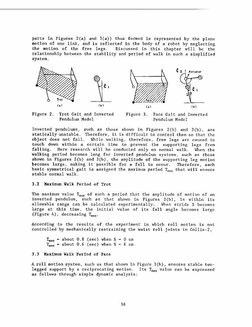
parts in Figures 2(a) and 3(a)) thus formed is represented by the plane motion of one link, and is reflected in the body of a robot by neglecting the motion of the free legs. Discussed in this chapter will be the relationship between the stability and period of walk in such a simplified system.

€1

(b)

Figure 2. Trot Gait and Inverted Pendulum Model

» 2 1 Actuator

(b)

Figure 3. Pace Gait and Inverted Pendulum Model

Inverted pendulums, such as those shown in Figures 2(b) and 3(b), are statically unstable. Therefore, it is difficult to control them so that the object does not fall. While walking, therefore, free legs are caused to touch down within a certain time to prevent the supporting legs from falling. Here research will be conducted only on normal walk. When the walking period becomes long for inverted pendulum systems, such as those shown in Figures 2(b) and 3(b), the amplitude of the supporting leg motion becomes large, making it possible for a fall to occur. Therefore, each basic symmetrical gait is assigned the maximum period Tmax that will ensure stable normal walk.

3.2 Maximum Walk Period of Trot

The maximum value Tmax of such a period that the amplitude of motion of an inverted pendulum, such as that shown in Figures 2(b), is within its allowable range can be calculated experimentally. When stride S becomes large at this time, the initial value of its fall angle becomes large (Figure 4), decreasing Tmax.

According to the results of the experiment in which roll motion is not controlled by mechanically restraining the waist roll joints in Collie-2,

Tmax = about 0.8 (sec) when S = 0 cm Tmax — about 0.6 (sec) when S — 6 cm.

3.3 Maximum Walk Period of Pace

A roll motion system, such as that shown in Figure 3(b), ensures stable two- legged support by a reciprocating motion. Its Tmax value can be expressed as follows through simple dynamic analysis:

38

• Support Im Lac

O Center of Gravity

Stride 1» lane

Moveeent of

the Center of Gravity

Initial Condition of

the Inverted Pendului

Figure 4. Relationship of Stride With Initial Value of Inverted Pendulum (Trot Gait)

* max — (2)

where:

i : length of supporting legs.

Tmax = 0.99 (sec) can be obtained when the physical amount t, =0.3 (m) of Collie-2 is substituted in the above equation. Tmax = about 0.85 (sec) was obtained in the experiment.

4. Maximum Movement Speed

When a = 0.5, movement speed VG can be expressed as follows:

2S (3)

As is indicated by this equation, an increase in movement speed VG is possible by increasing stride S or decreasing walk period T. Currently, maximum movement speed V^^ depends on the output limit Ulimit of the free leg driving actuator. The relationships of V^^ with S and T will be formulated below.

To swing a free leg forward over stride distance S, it is necessary to accelerate or decelerate it. The maximum value Umax of the inertia force compensating torque required at this time is proportional to stride S and counterproportional to the square of the walk period, as indicated by:

umtI = 48J x — (4)

39

where,

stride walk period length of free leg inertia moment of free leg

Umax must be smaller than Ulimlt. When equation (4) is substituted for umax < Ulimit, therefore,

fi • (5)

is obtained. This indicates that the upper limit value of the stride is a function of walk period T. Maximum stride Smax depends on the maximum period Tmax for stable walk, as described in Chapter 3 and as indicated by:

m"~ 487 *'Tm" (6)

When equation (5) is substituted for equation (3),

t/ ^ Ulimit , CT VC<^-x/xT (?)

is obtained. This equation indicates the following: in order to increase the movement speed, reducing the walk period is not expedient in achieving the maximum movement speed but, instead, it is desirable to maximize the period and stride. Stride S, however, cannot exceed twice the leg length. Therefore, restriction

S < 2i (8)

is given.

When walk period T does not exceed the maximum period Tmax, either of the following is given depending on whether Ulimit and J or t are large or small.

(1) Type-a: Smax < 2t since the actuator output limit Ulimlt is small.

In this case, the maximum movement speed Vg,^ depends on walk period Tmax (Figure 5 point-A), since the restriction condition of equation (8) can be disregarded. This can be derived from equation (7) as follows:

,, Ulimit I T

VGmox 24 J ( 9)

40

(2) Type-b: Smax > 2t, since actuator output limit UUmit is large.

In this case, a walk period

T-y[w^ (10) V "limit

that maximizes movement speed is given (Figure 5 point-B), since the stride is limited by equation (8) , and maximum speed V^^ can be derived as follows from equations (3), (8), and (10):

vw = /%p (11)

Collie-2 can be said to be of Type-a since Ulimit - 1.15 (nm) , J = 0.0153 (kgrn2) and t = 0.3 (m) and, when T = 0.8 (sec), Smax ■= 0.3 m. Dogs and other animals have been classified as Type-b since their stride has been observed to be constant, regardless of movement speed.

5. Movement Energy

5.1 Definition

In the case of walking robots, such as Collie-2, that obtain a large torque from large amounts of current using an electric motor, the most energy consumed during walking in Joule's heat loss represented by

E' = [tH^dt (12)

where, R£ = motor resistance, Gi = reduction ratio of gear, and KL - torque constant.

Torque (u^ can be obtained by solving the kinetic equation for walk trajectory. Here, the energy required per unit movement distance (movement energy) is represented by

VaT (13)

The many parameters used to plan the walk process can be obtained from employing the condition that movement energy P is minimized. Calculating the walk period so that the energy of movement at a certain speed will be minimized will be discussed here.

5.2 Calculation of Walk Period

P = C4+C^ + VVC + ^ (14)

is obtained (Appendix-1) when the movement energy P of a certain gait is expressed directly in terms of walk period T and movement speed VG, where the terms have the following significance:

41

First term: energy to swing free legs forward Second term: energy to swing legs up Third term: gravity-compensating energy dependent on the fall angle of the supporting legs Fourth term: gravity-compensating energy to support the body, including the free legs, of a robot

The values of the coefficients Csw, etc., of the terms of equation (14) for each gait can be obtained by dividing the P-value, calculated with equations (12) and (13), into elements (Appendix-1).

When dP/dT - 0 is solved using equation (14), T, in which P is minimized in relation to movement speed VG, can be obtained. Intuitively speaking, this is because an increase or decrease of walk period T causes an increase in stride S or free leg alternating current, resulting in an increase of the third term, or of the first and second term, respectively, of equation (14). Figure 6 shows the results of calculating basic symmetrical gaits.

1.25

«-. 1 u o

~ 0.75

0.5

0.25

0.2 0.4

Vo (m/Mc)

0.6

Relationship Between Walk Period and Maximum Stride

Figure 6. Relationship Between Movement Speed and Optimum Walk Period

5.3 Result of Movement Energy Calculation

Figure 7 shows the results of calculating the movement energy P for the trotting, pacing, and static walk (a - 0.75, crawl gait with leg movement delayed by 1/4 period) of Collie-2 using equations (12) and (13). The movement speed VG at the rightmost point of each gait or walk period indicates the maximum movement speed Vmax, as described in Chapter 4.

6. Experiment and Discussion

6.1 Experimental Results

Figure 8 shows photos of trotting and pacing. Figure 9 presents the results of trotting, pacing, and static walk experiments. The leftmost point of each gait or walk period indicates its maximum movement speed.

42

600

1 40° \

Q. 200

0.2 0.4 0.6

Vo (i/$ec)

0.8

Figure 7. Relationship Between Movement Speed and Energy (Result of calculating using equations (12) and (13).)

Trot gait

Pace gait

Figure 8. Photos of Collie-2 Walking

6.2 Influence of Walk Period

• Walk period and stability

As stated in Chapter 3, elongating the trot and pace period results in an increase in the roll movement amplitude, making the walk less stable. Specifically, when T is longer than 0.9 (sec), walk becomes unstable, frequently causing failure to occur.

43

1000

«00

1 too

\

400

200

D » D

A

Pie« B *

J O>0.5 D i 0.6

gtitle-Vfilk A:07 (1« |„ St«tle-V.lk) • X X 10.« (1.8 In SUtlc-talk)

* -' ■"■» (1.8 In Sutlc-V.lk)

lest T OiutabU

0.1

fa (•/•*) 0.2

Figure 9. Relationship Between Locomotion Speed and Energy (Experimental results)

• Valk period and maximum movement speed

As described in Chapter 4, an increase in the maximum movement speed Gmax occurs with the elongation of that trot and pace period. This is clearly shown in Figure 9.

• Walk period and movement energy

The walk period T - 0.8 (sec) that minimizes trot movement energy, according to the experimental results shown in Figure 9 (a - 0.55, V^^ - 0.1 - 0.15 (m/sec)), corresponds to a - 0.5, with a conversion value T - 0.72 (sec). It agrees with the calculated results shown in Figure 6.

6.3 Comparison of Gaits

• Gait and movement energy

The relationship between the gait and movement energy shown in Figure 9 is similar to that of the calculated results shown in Figure 7. For a low- speed gait, trotting is most advantageous with respect to movement energy.

• Gait and maximum movement speed

During static walk, maximum movement speed V^^ is very low since a cannot be smaller than 0.75. During trotting, on the other hand, the elongation of stable walk maximum period Tmax occurs upon increasing movement speed VGmax» as described in Chapter 3, so that maximum movement speed V^^ VGmax» as described in Chapter 3, so that _r .^^

Therefore, it is preferable that decreases, as described in Chapter 4. Therefore, it is pre: Collie-2 perform small movement energy trotting at safe speeds

7. Conclusion

In studying "stability," "movement speed," and "movement energy" as indices of four-legged walk, the authors concluded the following:

44

(1) The walk period considerably influences the indices. In order to increase the maximum movement speed, it is desirable to employ a long period and a large stride. They are limited, however, by the stable walk maximum period. A maximum movement speed walk period is given, as is a minimum movement energy walk period for a certain speed.

(2) Representative gaits are divided into trotting, pacing, and bounding. They exert substantial influence on the indices. Trotting is preferable at safe movement speeds, while pacing is preferred at other speeds.

Appendix 1: Induction of Equation (14)

The terms mentioned in 5.2 can be formulated based on the following assumption:

(1) Free-leg swinging-forward energy

When it is assumed, as described in Chapter 4, that the inertia-force compensating torque is proportional to stride and counterproportional to the square of the walk period,

E,wini = Const, x (=r) xT = C,w—=- T T (1.1)

(2) Free-leg swinging-up energy

When it is assumed, similar to (1) that the inertia-force compensating torque for a certain swinging-up altitude is counterproportional to the square of the walk period,

Eup = Const. x(±)*xT = Cu,±i

(3) Gravity compensating energy depending on fall angle of supporting legs

The body and supporting legs of walking machines basically require no acceleration/deceleration during normal walk, so the gravity compensating energy becomes dominant. If the gravity compensating torque applied to the supporting legs is assumed to be proportional to the stride when their fall angle is not very large, then

Esupport = Const, x S2 x T = CspT3VG2 (1.3)

(4) Gravity compensating torque for supporting walking machine's body, including free legs

If the gravity compensating torque of the body, including the free legs, is assumed to be nearly constant during the two-legged support pace period, then

Ebody " Const, x T = CbodyT (1.4)

45

The following equation is obtained from the above equation and (13).

Ec = Eswlng + Eup + Esupport + Ebody,

It has been confirmed through calculations that the assumptions described above are pertinent, and the coefficient Csw, etc., of equation (14) are nearly constant, regardless of movement speed VG and walk period T, in each of the basic symmetrical gaits, and that the following values have been obtained for Collie-2:

Csw , Csp Cbody AH(m) Cup(JS3)

(J/m2s) (Js3/m2) (J/s)

Trotting 80 650 0 0.005 0.18 Pacing 80 650 42 0.01 0.50

46

Development of Adaptive-Locomotion-Type Four-Legged Robot

43064062 Tokyo 4TH INTELLIGENT ROBOTS SYMPOSIUM PAPERS in Japanese 13/14 Jun 88 No 107 pp 45-49

[Article by H. Adachi and N. Kotaniuchi, Mechanical Engineering Research Institute; and E. Nakano, Tohoku University]

[Text] 1. Introduction

Recently concern has been growing in regard to the movement function of robots. Research is in full swing of conventional wheel-type robots as well as of legged ones that would exhibits excellent ground adaptability. The latter are divided into two-legged, four-legged, six-legged, and other types. Despite their potential, the problem with legged locomotion robots involves their complicated mechanism and control. The authors are now engaged in developing a six-legged fixed gait walking robot in order to solve this problem. Since a link mechanism is used to ensure the freedom of gate generation, basic control of leg motion is facilitated and importance is attached to environmental adaptation. Free gait systems, however, are advantageous for flexible walk. This paper will deal with a free gait type four-legged walking robot which the authors have developed.

2. Leg Mechanism

A number of walking robots have already been developed, with varying leg mechanisms. The supposition is that, since walking was originally a form of animal locomotion, the robot's leg mechanism should imitate that of animals. However, the authors do not believe that this imitation is always necessary since they do not involve the use of the same materials and actuators as living bodies. The robot developed here, therefore, employs a new "astballem" mechanism, as shown in Figure 1, for their legs. This three joint like-type mechanism has two degrees of freedom,each of which is connected to the link OA revolution 8 around point 0 of the variation in length of link OA. In Figure 1, the symbols "1," "s," and "B" denote the basic length, variable and the slide mechanism moving in a negative direction y-axially, respectively. Its most outstanding feature is that the C-point false linear motion can be ensured by applying either of the degrees of freedom. Figure 2 shows the path of its point-C that is obtained when (s) or 6 is changed from 1.0 to 2.4 or from -180° to 180° on the assumption that a = 300 (mm), 1 = 25 (mm), and k = 0.25. Figure 3 shows the

47

inclination of the path in Figure 2. As can be seen in the figures, the path is horizontal and nearly linear when (s) and 6 are within the range of 1.0 to 1.2 and ±50°, respectively. When the walking robot supporting leg motion is linear, the vertical motion of the robot is controllable. This can be ensured by applying either of the degrees of freedom. The self- support force separating-type leg driving mechanism is thus obtained, enabling it to walk with high energy efficiency. The above description suggests that the linear part is utilized for support period leg motion, and that 8 can be driven with an increased s-value during the resetting period. Figure 4 shows the influence exerted by the weight of the robot on its leg drive. During the support period, the robot's legs are subject to the reactionary force of the ground surface since it supports the body load. Part of it rotates link OA. If it is small, link rotation (0) is not influenced by the weight. It can be seen in the graph that the influence of the reactionary force of the weight is small when it is used for motion during the support period (the absolute value of 6 is comparatively small and the (s)-value is 1 to 1.2).

C(x,y)

Figure 1. Principle of Astballem

200 , , -I"" p 10o 200 rim.i

■-2.«

Figure 2. Trajectory of Point C

48

0.3 ,dy/dx

-0.3 -1.0'

Figure 3. Gradient of Trajectory Figure 4. Reaction Force Effect Some part of the reaction force of the robot weight becomes the force that rotates bar 0A. The axis of ordinates indicates (rotating force)/(reaction force).

The coordinate conversion equation and reverse conversion equation for the link mechanism are given below. If the coordinate of point-C in Figure 1 is denoted by (x,y), and

x - si sinö

y - si cosö - l(l/k-l) (k2a2-l2s2sin20)%

Their reverse conversion equations are:

s = (1/1) (p2 + q2)%

8 =■= tan"1 (p/q)

where: p - kx

q - y + (1-k) (a2-x2)%

3. Hardware

(1)

(2)

(3)

(4)

(5)

(6)

The authors experimentally manufactured a four-legged walking robot TURTLE-1, with an astballem mechanism, as is shown in Figure 2. It measures 500 mm in length, 330 mm in width, and 380 mm in height, and weighs 17 kg. The size of the link mechanism is: a = 300 mm, 1 ■= 25 mm, k=0.25. Figure 6 is a photograph of the link drive part. Each of its 2 degrees of freedom (0 and s) is driven by a DC servomotor. A ball screw is driven by a worm-worm wheel to vary value (s). Each driving part of (s) is rotated by a flat gear connected to a reducer to vary value 6. Values (s) and 6 are adjustable within the ranges 1-2.5 and ±90°. A leg extension mechanism is provided at the tip of the legs. A decrease in their length is possible

49

through the on-off control. However, this mechanism was not set on walk due to shortage of leg extension force.

Figure 5. Photograph of TURTLE-1 Figure 6. Photograph of Leg Driving Mechanism

The robot employs a potentiometer to detect angle (0) and length (s) of the link of each leg. Each of its motors has a tachogenerator. Its foot parts are fitted with a microswitch to detect contact with the ground surface and a force sensor to measure the leg load. Figure 7 is a photograph of the sensors. The force sensor utilizes the hole effect. In addition, it is fitted with a pendulum-type inclination angle sensor to measure its body posture.

Figure 7. Sensors Attached in Foot

CPU M

IM6/87 ,_,

Figure 8. Control System of TURTLE-1

50

Figure 8 shows the robot's control system, including the sensor system. It is controlled by a 16-bit personal computer. Its motor is driven by a motor driver with an analog speed control circuit. The speed instruction signal is transmitted to the computer from the motor driver. Software is used to control the position of the motor. Generally, the computer input/output is performed as follows: D/A 8 channels, A/D 22 channels, 4-bit digital input for the microswitch and 4-bit digital output for the leg extension mechanism The computer and motor driver are located outside the robot body ad interconnected by means of a cable.

4. Analysis of Gaits

When a robot is made to walk, it is first necessary to determine its gait. For this purpose, the following analysis is given: The gait of a four- legged robot can be described by four parameters if its phase alone is assumed to differ, although its legs draw the same path. The parameters include the duty factor (ratio of the time a leg contacts the ground during the walk cycle), as well as the phase difference among the other three legs as viewed from one leg. An examination of all combinations of phase difference is necessary in order for the gaits to be applied to a robot. Here, however, only bisymmetrical gaits will be examined. They are characterized by both the front and rear legs showing a phase difference of 0.5. This assumption is not thought unreasonable since walking robots and animals generally have a bisymmetrical structure. In analyzing gaits, the phase difference between the right front and left rear legs and the duty factor are denoted by <f> and ß, respectively (Figure 9).

s/2

-s/2 1.0

1 right front leg 2 left front leg 3 right rear leg 4 left rear leg

Figure 9. Feet Position-Time Trajectory The phase difference between 1 and 2 and between 3 and 4 is 0.5. <f> is the phase difference between 1 and 4 (or 2 and 3).

First, static walk requires the /3-value to be larger than 0.75. It has been learned while studying the gait obtained by varying the phase difference <f> that static walk is possible when:

ß < <f> < ß - 0.5 (7)

In other cases, static stability cannot be retained when the robot's center of gravity is located outside of the support polygon. Even if equation (7)

51

is satisfied, the stability allowance depends on the ^-value. represented as follows

sM - s (2ß + W - 2)/(2/3)

It can be

(8)

where (s) is the stroke. It is learned from equation (7) that the maximum allowance s(4^ - 3)/(2ß) can be obtained when <f> - ß - 0.5.

Semidynamic walk is such that the static support of the robot body by three legs during a portion of the walk period and by fewer than two legs during the remaining portion occur alternately. In this case, duty factor ß can take a smaller value than 0.75. However, its lower limit is 0.5. High- speed static walk is limited since the speed of the resetting legs must be more than three times that of the supporting legs. Semidynamic walk with ß less than 0.75 is possible at a high speed since the speed difference between the returning and supporting legs can be reduced. It has been learned in studying the gait obtained by varying <f>, as described in connection with static walk, that a gait suitable for semidynamic walk is obtained when

0 < (f> < ß - 0.5 (9)

In other cases of even three-legged ground contact, the center of gravity is located outside of the support polygon or support is performed by same- sided legs during a certain period. Same-side two leg support is not desirable since the experimentally-manufactured robot has no horizontal degree of freedom in the frontal lane. During two-legged support, the distance between the straight support line and the center of gravity of the robot is a minimum when <f> - ß - 0.5. The gait obtained at this time is believed to be the most suitable for stable walk. Figure 10 is a leg-timing chart obtained at this time.

iV£

1 right front leg 2 left front leg 3 right reer leg * left rear leg

Figure 10. Feet Position-Time Trajectory (ß - 0.7, 4, - 0.2)

During two-legged support, it is necessary to examine the dynamics of the robot since the position and posture of its body cannot be changed by the movement of the supporting legs. The motion of a robot, seen as an inverted pendulum, was calculated on the assumption that as it moves, it maintains

52

a certain altitude. For continued walk during two-legged support, it is necessary to set the following initial speed:

vx > (sx + s2) p/2

P - (g/h)%

(10)

(11)

where vx is the gravity center movement speed obtained when two-legged support starts, s1 and s2 are the positions of the front and rear supporting legs, respectively, (g) is the gravity center acceleration, and (h) is the altitude of the gravity center of the robot. During two-legged support, a robot moves as follows in the direction of its advance.

x ({2vx - p (Sl + s2)} ePfc

- {2vx + p (sx + s2)} e-PV^p) (12)

5. Walking Experiment

Figures 11-13 show the leg-tip force sensor output obtained during the walking experiment. The vertical axis indicates the load of the legs and the high-level part of the graph a loaded leg, i.e., a leg in contact with the ground. The scale on the vertical axis of the graph has no absolute significance because it is shifted to facilitate its read.

■A. /Ol Ml k» '«A' A A JK 1«8

.». 2. 3. «.5.

right rear

1«8

left rear

leg

time { 1 sec/dlv. )

walking speed ■troke

25 nn/aec 80 m

Figure 11. Output of Foot Force Sensor (ß - 0.8)

right front

time ( 1 aec/dlv. )

walking apeed stroke

30 Wsec 80 in

Figure 12. Output of Foot Force Sensor (ß - 0.75)

Figure 11 demonstrates static walk with ß = 0.8. It indicates that its support pattern has definitely changed. It exhibits the repeated cycles of six support patterns: 1) support by four legs; 2) support by three legs excluding the left rear one; 3) support by three legs excluding the left front leg; 4) support by four legs; 5) support by three legs excluding the right rear one; and 6) support by three legs excluding the right front leg.

53

right front leg

left front leg

right rear leg

left rear leg

tl»e ( 1 eec/dlv. )

walking epeed : 50 am/eee atroke : 80 nn/aec

Figure 13. Output of Foot Force Sensor (ß - 0.7)

Figure 12 shows the static walk with ß = 0.75. It also indicates that its support pattern has changed. It exhibits four support patterns: 1) support by three legs excluding the left rear one; 2) support by three legs excluding the left front one; 3) support by three legs excluding the right rear one; and 4) support by three legs excluding the right front one.

Figure 13 illustrates the semidynamic walk with ß - 0.7. It differs from the above two in that no distinct change of support pattern can be read. Ideally, the following support patterns are repeated: 1) support by three legs excluding the left front one; 2) support by the right front and left rear legs; 3) support by three legs excluding the right rear one; 4) support by three legs excluding the right front one; 5) support by the left front and right left legs; and 6) support by three legs excluding the right rear one. This is believed to be attributable to the following: the robot is not absolutely the same as the model (inverted pendulum), the motion of the returning legs causes force to be exerted on the robot's body so that it loses its balance, and a leg that should originally have risen above the ground surface moves along it due to its slow vertical motion. As is seen in Figure 13, two-legged support occurs distinctly and semidynamic walk is performed.

6. Postscript

The authors experimentally manufactured a free-gait-type four-legged walking robot and studied the gaits for possible application. They proposed a walk form termed semidynamic walk, and evaluated it, as well as static walk, in respect to leg load. The robot had many restrictions due to its low degree of freedom. They would like to continue studying walk in the future using a high freedom level.

54

Research of Thrust-Powered Wall-Surface Walking Robot

43064062 Tokyo 4TH INTELLIGENT ROBOTS SYMPOSIUM PAPERS in Japanese 13/14 Jun 88 No 108 pp 51-55

[Article by A. Nishi, Miyazaki University]

[Text] 1. Introduction

The author designed a robot capable of performing safe locomotion on a rough wall surface at a high speed. Provided with a thrust motor, combining an engine and a propeller, and with a small jet engine, it utilizes the frictional force obtained when its vehicle with wheels or crawlers is pressed against the wall surface, with the thrust power working line inclined toward the wall surface. He has also studied the thrust motor's characteristics and design conditions that are required when a robot with such a mechanism moves along the rough surface of a vertical wall, such as the outer wall of a multistored building. First, this paper will describe the safety conditions required for oblique locomotion along the wall surface and the advantages of a wheel drive. Next, in order for the robot to move safely along the wall surface of a multistoried building, it is necessary to give due consideration to the influence of the wind. The wind resistance of the vehicle influences its shape. Therefore, the former can be calculated experimentally when the latter is determined. On the other hand, the inclination of the thrust motor is changed when the robot is controlled. Therefore, it is necessary to experimentally examine the wind influence on the thrust motor. In general, the wind velocity changes randomly, so the thrust motor's resistance to its power spectrum is being examined. The characteristics of the thrust motor depend on the inertia moment of the rotary part and the air flow within. Large and small ones, therefore, have different characteristics. Here the resistance variation obtained to the velocity of the air in a wind tunnel will be measured using a small thrust motor model, the results of which will be used to examine its characteristics, and control will be studied in order to secure the safety of the robot on the wall surface.

55

2. Conditions for the Safety of Robot on Wall Surface

2.1 Oblique Movement

Since insufficient thrust power is generated, the minute control of a vehicle is necessary to prevent it from falling during oblique locomotion. First, it is necessary to decrease the probability of engine failure by providing two thrust motors. The mutually opposite torques applied can be canceled by rotating the engines opposite each other. The model in Figure 1 was assumed to be such a two-engine type. It was designed to be capable of obliquely moving along the rough wall surface of a building when its wheels were brought into contact with the tip of a rise and when all of them were inclined at the same angle.

Figure 1. Relationship of Wheel Inclination and Thrust Power of the Model

If the inclination angle of the wheels, that of the combination thrust power and that with the wall surface of the combination thrust power obtained when the wheels are not driven are denoted by 8, a, and 7, respectively, the formula for the balance between the force in the same direction as the inclination of the wheels and that orthogonal with it are given as follows:

Tcos 7 cos (0 - a) > W cos 8

Wsin 8 - Tcos 7 sin (8 - a) < fi Tsin 7

(1)

(2)

where fi is the coefficient of the friction of the wheels with the wall surface in the same direction as the axles of the vehicle. Both formulae can be converted as follows:

COid uv cosy cosre-m)

W MSihß T cosr iir>(&-&)

(3)

(4)

T can be minimized when 8 - a.

7 - tan"1 (tan 8/p) (5)

56

Formulae (3) and (5) are shown in Figure 2.

Figure 2.

6(f. Kf«f

Relationship Established Among 7, 9, and T/D When Wheels Are Not Driven

2.2 Wheel Drive

The driver's weight was increased since it drives the wheels. This is advantageous in some cases because it is capable of converting the force component of the wall surface pressing direction into thrust power. Combination thrust power is given by equation:

TR/T = cos 7 + n sin 7

The maximum value of TR is given as follows:

7 = tan-1 n

(6)

(7)

7 < 45° when p is generally smaller than 1. The relationship between y. and 7 in equation (7) and TR/T in equation (6) are shown in Figure 3. When n is large, TR/T is large.

*n r 1.5 ■ 50*

u / 4tf

13

/ /

30*

12 / / 20*

1.1

10 (

/ y

/ y

■ 10"

) 02 0A 06 OB V '

0

Table 3. Wheel Driving Combination Thrust Power

57

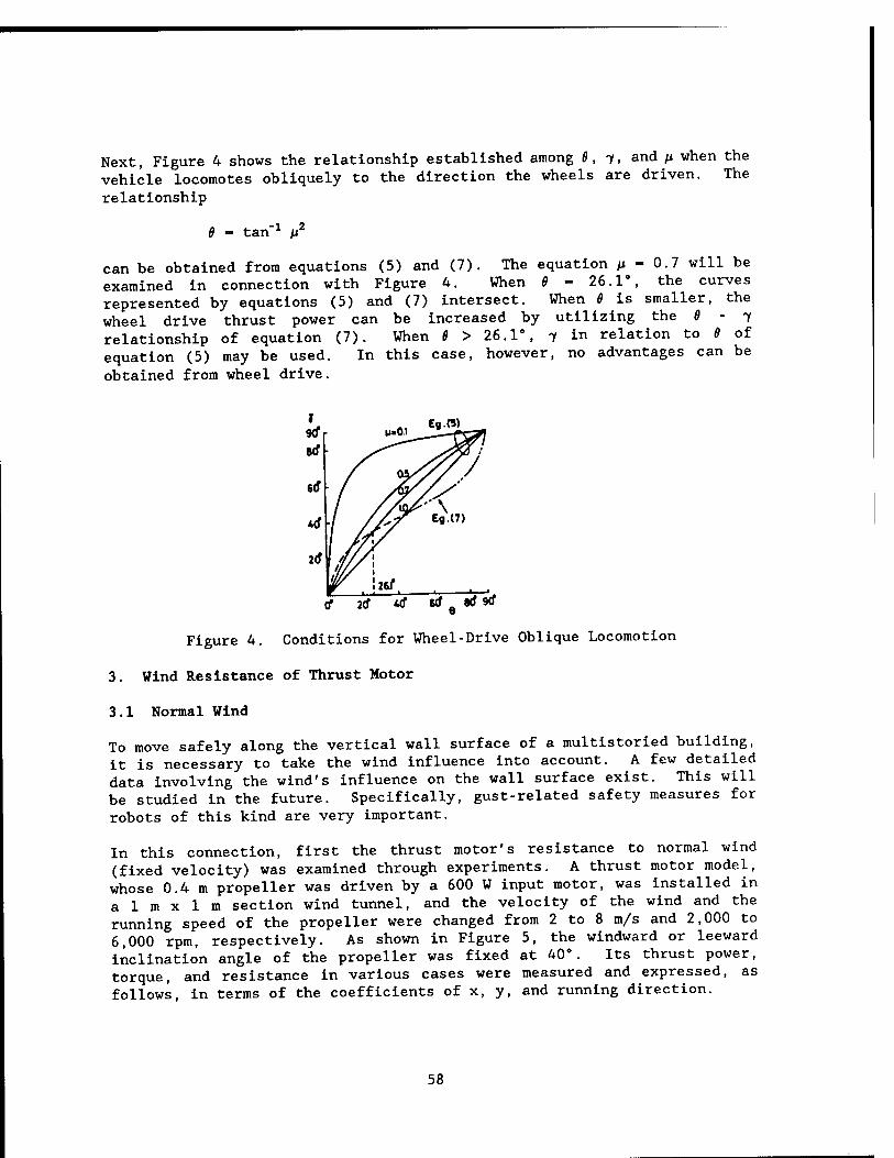
Next, Figure 4 shows the relationship established among 6, 7, and /x when the vehicle locomotes obliquely to the direction the wheels are driven. The

relationship

6 - tan"1 /i2

can be obtained from equations (5) and (7). The equation /i - 0.7 will be examined in connection with Figure 4. When 6 - 26.1°, the curves represented by equations (5) and (7) intersect. When 6 is smaller, the wheel drive thrust power can be increased by utilizing the 6 - 7 relationship of equation (7). When 6 > 26.1°, 7 in relation to 9 of equation (5) may be used. In this case, however, no advantages can be

obtained from wheel drive.

t 9rf M»0.1

Eg.(5)

- /

/■*/ E9.(7)

id 1 l// \w 2if . cf 2rf *rf 6tf . 8tf 9tf

9

3.

Figure 4. Conditions for Wheel-Drive Oblique Locomotion

Wind Resistance of Thrust Motor

3.1 Normal Wind

To move safely along the vertical wall surface of a multistoried building, it is necessary to take the wind influence into account. A few detailed data involving the wind's influence on the wall surface exist. This will be studied in the future. Specifically, gust-related safety measures for

robots of this kind are very important.

In this connection, first the thrust motor's resistance to normal wind (fixed velocity) was examined through experiments. A thrust motor model, whose 0.4 m propeller was driven by a 600 W input motor, was installed in a 1 m x 1 m section wind tunnel, and the velocity of the wind and the running speed of the propeller were changed from 2 to 8 m/s and 2,000 to 6,000 rpm, respectively. As shown in Figure 5, the windward or leeward inclination angle of the propeller was fixed at 40°. Its thrust power, torque, and resistance in various cases were measured and expressed, as follows, in terms of the coefficients of x, y, and running direction.

58

Cx -

C, -

C% -

D- Tsinft

Ttos/3

a i:?^S

(8)

where T is the thrust power (N) orthogonal to the propeller surface, D is the resistance (N) in the same direction as the wind, Q is torque (N«m), V is wind velocity (m/s), S is the area (m2) of the propeller, R is the radius (m) of the propeller, p is the density of the air (kg/m3), and ß is the angle of Figure 5.

Figure 5. Inclination Angle of Model

It is learned from Figure 5 that a slight deflection of the air current in the wind tunnel results in slight resistance of the propeller when it is inclined windward (ß > 0). When the inclination is leeward, the air currents behind the P and in the wind tunnel run counter to each other (ß<0).

Figures 6(a), (b), and (c) show Cx, Cy, and Cq, respectively. On windward inclination, Cx is expressed in terms of negative values since the horizontal axis component of the thrust power of the propeller is larger than the resistance, so the combined force is directed windward. When ß < 0, Cx is expressed in terms of positive values since both the thrust power and resistance are directed leeward. Horizontal axis A = u/v, where (u) is the circumferential speed of the propeller, and its practical values are 200 - 300 m/s. A = about 10 - 30 if the velocity (v) of the wind at the wall surface of a building is assumed to be 10 - 30 m/s. Cx values are arranged in the order of the inclination angle of the propeller indicate that the resistance depends on the inclination angle.

Cy corresponds to A ß = +20 Ag or +30°.

about 10, a very small value when compared to

The torque coefficient Cq does not vary much with ß.

3.2 Relationship Between Thrust Power and Resistance

Figure 7 shows the relationship between thrust power T and resistance D, confirming the wind velocity range at which a robot of this type is safe on the wall surface of a building and the propeller inclination range.

59

Figure 6(b). Force Component Orthogonal to Wind

20 30 x«u/v

Figure 6(a). Force Component in Same Direction as Wind

to

8 //' tf

t /fV3*

4 /

2

/

so n \

Figure 6(c). Torque Component

Figure 7. Thrust Power to Resistance Ratio

60

T/D - 4 - 20, 4 - 15 or 4 - 8 when A - 10 - 30 and ß - +30°, +10° or -30°, respectively. The thrust power exhibits a value more than four times that of resistance in all cases, and the possibility exists of securing safety by properly adjusting the thrust power angle.

3.3 Side Wind Safety Conditions

As is clear from the experimental results described above, different resistances work depending on the fitting angle of the thrust motor when a side wind is present.

When the thrust motor and vehicle have side wind resistance D, it is assumed that the latter's safety is secured by increasing thrust power T and wall surface side inclination angle 7, as shown in Figure 8, based on the variation of T/D described above. Side wind resistance D is decomposed into the component in the thrust direction (same as the inclination angle of wheels) and that orthogonal with it, and the newly-required thrust power and side wall inclination angle are denoted by T' and 7', respectively, giving the following force balance conditions:

T'cos 7' > Wcos 6 = Dsin 6

H T'sin 7' > Wsin 9 + Dcos

From this we obtain:

( 1 D/v (D/w)tan6 j

T' > C6S8 -t (DAv)smg W COSTS'

(9)

(10)

(11)

(12)

M =c> %■

w

Figure 8. Relationship Between Forces Obtained With Side Wind

The following can be derived from formula (3):

T \ cosg) W cos $

(3)'

61

when 6 - a (in this case, it is assumed that a - ß) . Therefore, in formulae (11) and (12),

D ^ D cose WTcostf (13)

Control rates A7 and AT/W are obtained from:

-tarf(t<vn0/,u) (14)

£T.IT.JL2 fos6*cyr)(ttfteMy) .ton. w ~ w" w - cosr' c*sr /15s

As shown in Figure 7, T/D values are experimentally given for A. Therefore, A is specified for a certain wind velocity when the circumferential speed of the propeller is known, and T/D can be calculated when the inclination angle ß of each thrust motor is given. Therefore, the increment of the required thrust power and the increment A7 of the inclination angle 7 of the thrust in the same direction as the wall surface can be obtained from formulae (14) and (15).

3.4 Thrust Motor Resistance to Abnormal Wind

The resistance of the thrust motor to an abnormal wind whose velocity varies hourly has been obtained through experiments. The blower in the wind tunnel is controlled by an invertor. Controlling the wind velocity to within a certain range is possible through the use of a computer.

This time the variation of the resistance, torque, and thrust power of a thrust motor in a nearly sine waveform at range V - 4 - 8 m/s was measured. The examples of the results of this measurement, conducted when the propeller was fitted at +30°, 0°, and -30°, are shown in Figure 9. The absolute values of the resistance obtained in this case do not correspond to the results mentioned above since it is orthogonal to the thrust power. All curves, however, show little time lag corresponding to wind velocity. This example is obtained when the wind velocity variation period is 4 seconds. Longer periods provide similar results.

The model used for the test was small and shows a very high frequency characteristic since the inertia moment of its rotary part is small. Since an actual thrust motor is large, however, it would show a correspondingly- long time lag. The following has been learned from the above description the air force exerts such a small influence on the propeller the thrust power and resistance waveforms are only slightly deformed. However, this is not believed to cause any great time lag.

In this case, the time lag of the wind tunnel's blower and the limits of the invertor performance prevented the test from being continued. However, in the future we plan to make the thrust motor capable of higher frequency performance, required for higher resistance to actual wind.

62

X«)

Wind Velocity

Thru*!

S^öp-*-

Figure 9. Abnormal Wind Characteristic of Thrust Motor

In light of the test results described above, it can be said that the brief time lag of the thrust motor model with respect to wind velocity variation, with a period more than 4 seconds, and its dynamic thrust power and resistance variation can be explained in terms of its static characteristics.

The wind that is in direct contact with the front side of a building wall and the rear current side wind that is in contact with the back of the building, on the other hand, are thought to have much different characteristics. The latter's velocity is believed to show a large variation, while the former's shows a small variation, even when it is high. The low- and high-layer components of wind are believed to exhibit quite different characteristics. Their measurement and examination will be necessary in the future.

4. Wind Safety Measures

The safety of robots of this kind will be examined based on the abnormal test results described above. First, wind velocity is assumed to undergo the same v = 4 - 8 m/s sine waveform variation as that in the test. If the period of wind velocity variation is fixed at more than 4 seconds, the static characteristics in Figure 7 are directly applicable. A = (u/a)cosec wt if v - a sin wt is assigned to A = u/v in Figure 7. Figure 10 shows an approximation of T/D for A ■= 10 - 30, and required control rates A7 and AT/W obtained from formulae (14) and (15) for 6 - 20° and p = 1.0.

This example illustrates the resistance variation of a single thrust motor. If there are multiple thrust motors, it is necessary to take the corresponding increase in wind resistance into account.

An important task for the future will be to estimate the actual variation in wind velocity.

63

*rw«t)

Figure 10. Variation of Abnormal Wind Control Rate

5. Conclusion

The basic design specifications of a robot capable of high-speed locomotion along the outer surface of a building have been derived and strong wind safety measures examined as follows:

(1) The locomotion conditions along a vertical wall surface are derived.

(2) Wheel drive safety conditions are derived.

(3) Thrust motor resistance to normal wind derived through experiment.

(4) Thrust motor resistance to velocity-varying abnormal wind derived through experiment. As a result it was learned that the model caused no more than a 4-second time lag.

(5) Control rate can be calculated using static characteristic values when time lag is small. The examples of this calculation are described above.

In the future we will define the properties of the wind striking the wall of a building.

64

Development of Wire-Suspended Robot

43064062 Tokyo 4TH INTELLIGENT ROBOTS SYMPOSIUM PAPERS in Japanese 13/14 Jun 88 No 109 pp 57-62

[Article by T. Tsujimura and T. Yabuta, NTT Transmission System Research Institute: "A Mobile Robot Walking on an Aerial Path"]

[Text] 1. Introduction

Communications cables are roughly divided into aerial and underground ones. During the former's stretching or maintenance, workers are required to climb to an altitude of several meters above the ground. The automation of construction and maintenance is desired to liberate humans from such dangerous work and increase work efficiency.

Aerial cable stretching and maintenance robots locomote along trajectories and work using hands or the like at prescribed posts. The elementary techniques required for them include a manipulator, and measuring and locomotion techniques. Several systems are used for locomotion. The simplest among them are those which perform rotational locomotion along trajectories, such as wheels. Telephone cables generally have metallic fittings. The locomotion of wheel-type devices becomes unstable due to the vibration, etc., generated when rolling over these fittings. Legged-type locomotive devices, on the other hand, are capable of stepping over obstacles, eliminating their unfavorable influence on the locomotion characteristics.

The locomotion technique is applicable to flat surfaces, stairs (1), wall surfaces (2), ducts (3,4), etc. A few reports have, however, been published on robot locomotion along the trajectory of a one-dimensional line in the air, such as aerial cables, which is dealt with here. Wheel, leg (5-10), crawler, and other locomotive devices have been proposed previously. Many reports (6-10) have been published specifically on the two-dimensional surface walk of robots with two- and four-legs and other structures. In connection with leg-type locomotion, much research has been conducted recently on controlling dynamic walk. The authors' study, on the other hand, deals with static locomotion in consideration of the characteristics of the work environment. The optimal design of the mechanisms to provide the desired operation has been pursued in order to minimize control cost.

65

This paper will describe the methods and mechanisms for stable locomotion along a one-dimensional trajectory, with obstacles, in the air. First, a method for stable locomotion along a trajectory will be discussed and an appropriate mechanism will be proposed. Second, a suspended locomotion mechanism with slider crank mechanism legs will be designed and kinematically analyzed. Finally, the locomotion performances of the locomotive device will be evaluated, and an optimal design method, planned to secure its stability during locomotion, will be presented.

2. Principle of Locomotion

Communications cable are generally stretched in the air as follows. Steel- wire suspension cables are stretched between poles and communications cable bodies are suspended on them using metal devices. A communications cable maintaining and inspecting system has been designed to move along the trajectory of a suspension cable stretched in the air. The metal devices are generally installed at equal distances. Here, they serve as obstacles to be stepped over by the locomotive device.

The continuous rolling of blocks, etc., is effective for moving along a trajectory without obstacles. Some systems for winding optical fiber cables around power cables have mechanisms for the block locomotion on power cables (12). Existing communications cables, on the other hand, have such locomotion obstacles as suspenders, connecting terminal blocks, etc. Therefore, a device must step over them during locomotion. Legged walking systems that intermittently repeat connection and disconnection actions are preferable over wheel systems that remain in contact with the trajectory during locomotion, as described above, for stepping over obstacles while maintaining their stability. Stable locomotion is significant for legged walk. The device is suspended on a trajectory. Its gravity center, therefore, is located below the trajectory, so it readily maintains its stationary stability. During locomotion, on the other hand, its stability depends on its motion. This will be described in Chapter 4.

The motion of a walking system consists of standing and free leg phases (5). Walking is performed by alternately repeating the phases. At least 2 degrees of freedom are generally necessary. Degrees of freedom generally involving combinations of turning and extension joints. A mechanism of the human upper and lower leg type is constructed by arranging turning degrees of freedom in series. In this case, an actuator, corresponding to the degrees of freedom, is generally provided, so its structure is large and very complicated control is necessary.

A mechanical method, not a control method, is used to ensure two walking phases. When a mechanism (13) such as a link, cam, etc., is used, one turning input can approximately be converted into two walking phases. Some links are applied to walking machines (14-18).

Proposed here is a system which locomotes along a straight trajectory in the air using a link mechanism and only one actuator. It employs a DC motor, as shown in Figure 1. Its driving force is transmitted to the front and rear legs by the chain and sprocket. Each leg consists of two slider crank

66

mechanisms, OABLCL and CABRCR, as shown in Figure 2. Arm links BLCL and BRCR are employed for locomotion, and a gripper, fitted at their tips, is suspended on a trajectory to support their weight. The angle formed between links ABR and OA that constitute slider crank CABRCR is defined as input rotation angle 9. The phase difference between the two slider crank is assumed to be the 7r-radian. In an ideally-designed slider crank mechanism, the input turning angle (0) of the free leg phase is as follows:

0 < 8 < n/2, 3/2w < 8 < lit,

and that of the standing legs is as follows:

TT/2 < 0 < 3/2*.

The system locomotes as follows. As shown in Figure 3, it uses the x-axis of an xy-coordinate system as the trajectory. The initial position of the system is obtained when 8 is fixed at 0, and link end C2L is positioned at its origin at time (t) = 0. At this item, CR, CL, 0, BR, A, BL line up along the y-axis in order. First, the gripper CR passes CL, coming into contact with the trajectory when arms BR, CR locomote, with CL remaining at the origin. Next, gripper CL leaves the origin and passes CR. The cycle of operation described above, i.e., the contact and separation of the gripper at the tip of the arm oh and from the trajectory, are alternately repeated during locomotion. During iimit. grippers CL and CR each come into contact with the trajectory at only one point per cycle. Locomotion during which obstacles can be stepped over is possible, if arm trajectories are planned sufficiently. The ideal trajectories of the arms are of the closed curve type and involve a linear standing phase. They can be designed based on the results of analyzing the motion of the slider crank mechanisms that constitute the arms. This method has been designed to present ideal arm trajectories without complicated actuator control by using a mechanical function, thereby reducing control costs.

Trajectory of Leg End

/ \

Sprocket

DC Motor Chain

Figure 1. Suspended Locomotion Figure 2. Slider Crank Mechanism

67

0 =3TT

Figure 3. Leg Motion

Suspended Locomotors

The motion of the suspended locomotive device mentioned in the preceding chapter will be described here, with (a), (b), and (c) denoting the lengths of links OA, ABR, BRCR, respectively. Link OA, however, is assumed to locomote constantly, parallel with the y-axis. The two slider cranks that constitute a pair of legs alternately repeat the standing and free leg phases. When they are set to have different w-radian phases, one of them is always entering the standing leg phase to come into contact with the trajectories.

Discussed here will be the motion of a pair of legs along a straight line y - 0 trajectory in a rectangular coordinate system such as that shown in Figure 3. It is assumed that the slider cranks have been set in operation with the input turning angle fixed at time function 6 - 9 (t). CL or CR is at a fixed point on trajectory y - 0 when -7r/2 + 2n*r < 6 < n/2 + 2n?r or it/2 + 2n7r < 6 < 3/2TT + 2mr, respectively, where (n) is 0, ±1, ±2, •••, and it is referred to in positioning the legs. In this condition, the motion of the legs and trajectory of link ends CR, CL are shown in Figure 3.

When the input link rotates at constant speed w, the turning angle, angular velocity, and angular acceleration at time (t) can be presented by the following equations, respectively:

6 - wt d0/dt - w d20/dt2 - 0

(1) (2) (3)

The motion of the system will be expressed in terms of the reference point- 0 of the legs in Figure 2. Its coordinate at time (t) is represented by equations

x - (-l)m b(l-c/b(a2/b2+l +2(-l)m a/b coswt)"%)sinwt

+ 2mb(l-c/b(a2/b2+l)~%)

y - b(l-c/b(a2/b2+l+2(-l)m a/b coswt)-*) • (-l)m coswt+a/b)

(4)

(5)

where (m) is an integer as given in formula ut/n - 1/2 < m < o)t/ir + 1/2,

68

Figure 4 shows the locomotion route obtained using the above equations in which (c) was changed as a parameter, with a = 1.6 and b = 1 assumed. The curve above or below the x-axis represents the trajectory of link end CL or system body reference point-0, respectively.

Trajectory a=i.6 b=i

c=11 Leg End

-25

Figure 4.

Body' -10^

Trajectory of Suspended Locomotive Device

The locomotion of the system can be obtained, as follows, when the above equation is differentiated by time:

dx/dt = (-l)m b (coswt-(-l)m c/b (a/b + (-l)m (a2/b2+l) coswt +a/b cos2wt) • (a2/b2 +1 +2(-l)m a/b wt)"3/2) w

dy/dt = (-l)m b(c/b (a2/b2+l+2(-l)m a/b coswt)"3/2

• (1 +(-l)ra a/b coswt)-l) sinwt w

(6)

(7)

Figures 5 and 6 show the locomotion velocity obtained using the above equations. The former indicates the x-velocity obtained using c/b as a parameter when the link ratio a/b -1.6 (constant). The values obtained by normalizing time by the turning angle velocity w of the input link and those obtained by normalizing locomotion velocity by the product of link size (b) and angular velocity u> are taken for the horizontal and vertical axes, respectively. Figure 6 indicates the y-velocity obtained when a/b = 1.6. It has value-0 when the time is 0 or ww, or the maximum or minimum value when the item is l/2itu> or 3/2™, respectively.

The locomotive acceleration of a locomotive device is given, as follows, by differentiating the above equations by time:

d*x/dt'=H)* b (c/b (1/4 (aVb»+1+2(-l)" a/b costut)» +3/4(aVb'-l>» }

■ (aVb2+l+2H)" a/b coscut)"5'2-1) «incut w»

d*y/dt*=H)" b ( (c/b (tVb»+l+2H)" a/b coswt)-"'- (1 +(-|) - a/b eoswt)-)) coswt

+ H)-a/b -c/b (a'/bs+|+2(-|)- a/b coswt)-"»

• (2-aVb* +H)" a/b coswt) sin'wt ) u1

(8)

(9)

69

X-VELOCITY a/b=1.6

27t

TIME x Cü

Figure 5. X-Velocity of Suspended Locomotive Device

-2

X-ACCELERATION a/b = 1.6

2n

TIMExW

Figure 6. Y-Velocity of Suspended Locomotive Device

Figures 7 and 8 show the locomotive acceleration obtained using the above equations. The former indicates the x-acceleration obtained when a/b -1.6. The x-velocity takes value-0 when the time is 0 or 7rw, or the maximum or minimum value when the time is 1/2TTW or 3/27rw, respectively. The latter, on the other hand, expresses y-acceleration. Its total absolute value becomes a minimum when c/b - 6.6.

Y-VELOCITY a/b = 1.6

Y-ACCELERATION a/b = 1.6

TIMEx W TIMExw

Figure 7. X-Acceleration of Suspended Locomotive Device

Figure 8. Y-Acceleration of Suspended Locomotive Device

The locomotive characteristics of the locomotive body derived from the motion of the slider crank mechanism constituting the legs will be evaluated to examine its locomotive stability. This depends on the behavior of the arm tip during the standing leg phase. The longitudinal and vertical motion of a locomotive body can be seen by analyzing the relative motion of the arm tip on the coordinate system peculiar to the slider cranks. For this reason, the locomotive stability of a locomotive body can be evaluated by examining the motion performed by the arm tip in a fixed position.

The ideal locomotion of a locomotive body occurs along a trajectory at a constant velocity. In this connection, therefore, 1) the vertical motion of a locomotive device: orthogonal to trajectory; and 2) inconstant trajectory motion, during the locomotion of a locomotive device will be examined here.

70

4.1 Vertical Motion

The oscillatory motion orthogonal to the trajectory of a locomotive body can be evaluated in terms of the nonlinearity of the path and of the vertical velocity and acceleration of the arm tip.

The vertical oscillation during the locomotion of a locomotive body reduces to its optimum value when the tip path of the arm of the slider crank mechanism in Figure 2 becomes increasingly straight and parallel with the x-axis, when 7r/2 < 6 < 3/2n. The linearity of the path during the standing leg phase is defined as

ATsd/K/^Udy/dflj/Wx/dfl})» iß)<» (10)

This is illustrated in Figure 9, with link length ratio c/b and AT taken for the horizontal and vertical axes. The above equation represents the mean square of the inclination of the path. When a/b = 1.6 and c/b = 6.6, AT becomes a minimum and the arm path becomes most similar to a straight line.

Figure 9. Locomotive Stability Based on Locomotive Path

The y-velocity of the arm tip is obtained when the locomotive body oscillates vertically. Its optimum value is 0. For the purpose of its evaluation, it is defined as follows:

AVy= (1/n/^"(dy/dt)' do)1" (11)

Figure 10 shows the value of the y-velocity when the input turning angle velocity is kept constant. Since it is small, the vertical oscillation is also small, providing high stability. Value A Vy is a minimum when a/b =1.6 and c/b = 6.6.

The y-acceleration of the arm tip is defined as follows:

AAy= (1/7t/^"Vy/dtV do)"1

(12)

Since the value is small, vertical oscillation is small, providing a high stability. As shown in Figure 11, value AAy is a minimum when a/b - 1.6 and c/b =6.6.

71

0.5

Figure 10. Locomotive Stability Based on y-Velocity

Figure 11. Locomotive Stability Based on y-Acceleration

4.2 Movement in Trajectory Direction

The inconstant movement in the trajectory direction is caused by the inconstant velocity or acceleration of a locomotive device. It can be evaluated in terms of the velocity and acceleration of the arm tip.

The average x-velocity Vx of the arm tip is defined as follows:

Klt (13)

Velocity variation is defined, as follows, using the mean velocity value Vx and the mean square of the difference between the velocities of each point.

AVx= (l/Tt/^Wdt-Vx)' dfl)'" (14)

This is shown in Figure 12. Since value AVx is small, the velocity is highly constant, stabilizing locomotion. The locomotion velocity variation is the smallest when parameter c/b is 6-7.

Acceleration is 0 when the arm tip moves at a constant velocity. Acceleration occurs when the velocity varies. The instability of movement can be evaluated in terms of acceleration.

AAx= (]/,t [3""{i'xm')> do)"» (15)

72

1 a/b= -1 2

~ 0.8 1.6—7 /

? 0.6 .o

> 0.4 < ^ 0.2

2.0-7// /

2.4~\

°( 2.8 -^

> 6 10 15 2

c/b

Figure 12. Locomotive Stability Based on x-Velocity

As shown in Figure 13, value AAx is small, providing high stability since value a/b is large.

0.5

« 0.2

Figure 13. Locomotive Stability Based on x-Acceleration

It has become clear from the above description that the locomotive velocity is highest when the link ratio a:b:c of the slider link is 1.6:1:6.6.

5. Conclusion

Basic study was conducted involving a robot locomotion technique necessary for developing an automatic system to stretch and maintain aerial communications cables.

(1) A locomotion method that ensures the step over of obstacles on the trajectories and its mechanism were proposed. This proposal makes locomotion easier than that involving legs which is carried out by controlling a number of actuators.

(2) A suspended locomotive device, whose legs employ a slider crank mechanism, that performs approximately linear motion has been designed and the locomotion of the locomotive body has been formulated kinematically.

(3) The locomotion stability of the suspended locomotive device has been determined by analyzing the motion of the slider crank mechanism and evaluating its oscillation caused by the velocity, acceleration, etc., of the link. As a result it was learned that the link ratio of the slider link crank mechanism that ensures most stable locomotion is 1.6:1:6.6.

73

Development of Wheeled Wall Surface Walking Robot

43064062 Tokyo 4TH INTELLIGENT ROBOTS SYMPOSIUM PAPERS in Japanese 13/14 Jun 88 No 110 pp 63-68

[Article by T. Sato, T. Fujisawa, Y. Tanaka, and A. Hagio, Nippon Kokan K.K.]

[Text] 1. Introduction

There is a growing tendency to automate the inspection and repair aspects involved in maintaining oil tanks, globular tanks, and other large plant structures, as well as ships and vessels. Robots used for this purpose would move while adhering to the wall surface. They are, therefore, called wall surface walking robots. Study and development is now underway regarding robots employing a variety of adhesive and locomotive mechanisms.

The adhering-walking systems of wall surface walking robots can roughly be divided into wheel and crawler walking systems, with built-in permanent magnets, and vacuum walking systems (there are also intermediate type ones). The former require no suction energy and show a high locomotion velocity. However, their disadvantages are as follows: the wheel systems are not capable of generating any substantial adhesive force and crawler ones are not suitable for spherical and stepover walk. On the other hand, the latter's strength is that it is capable of generating a large adhesive force, but its weakness is that its operation is performed intermittently and slowly. The systems function opposite to each other. The choice between them should be made after taking application purposes, environmental conditions, etc., into account. They are applied to structures with varied curvatures, such as cylindrical and spherical ones. None of the aforementioned systems are applicable to all wall surface shapes.

The authors have developed a walking robot with a permanent-magnet wheel system and a constant adhesive performance that is applicable to various wall surface shapes of steel structures. It will be summarized here.

2. Principle of Development

The robots must offer the following characteristics for the flaw detection, cleaning, painting, etc., of large structures.

74

(1) Capable of free locomotion, maintaining stable adherence to wall surface.

(2) Applicable to fault, curved, and spherical surfaces, as well as surfaces with steps, such as weld beads, etc.

(3) Will not damage the coat of the wall surface.

(4) Capable of maintaining safety, even during power failure or other unexpected accident.

(5) Capable of being self-standing.

Specifically, items (1) and (2) can be said to be the most important functions for increasing the automaton and efficiency of various kinds of inspection and other jobs.

In this study, the authors developed a highly universal wall surface walking robot, setting up the aforementioned five items as development targets, and employed a magnetic adhering wheel walking system with a permanent magnet as the basic mechanism attain the targets.

3. Structure of Wheeled Wall Surface Walking Robot

3.1 Overall Construction

The robot consists of a walking system with four sets of magnetic adhering wheel units and two DC motors for driving two sets of right and left wheels, a probe for inspection purposes, an arm to conduct various jobs, gripping, cleaning and painting devices, a TV camera monitor, sensors (walking range finder and posture detecting inclinometer) to provide information about the robot's status, and a controller to control the walking of the robot and the operation of the arm.

In order to decrease the weight of the system body, the basic structure has been simplified and its main part is mostly composed of hard aluminum. Its steering is performed toward the low-speed side by giving a speed differential to the right and left systems of the wheel units. This structure is also aimed at structural simplification and weight reduction. Figure 1 shows its appearance and Table 1 the main specifications of the walking system.

3.2 Wheel Structure

The magnetic adhesive wheels with built-in permanent magnets have a structure in which a hollow disk magnet is placed between two disk yokes. Therefore, only the yokes come into contact with the adhesive object surface, and no load is imposed on the brittle magnet. This is of rare earth cobalt, with high magnetic characteristics. The wheel structure is shown in Figure 2.

75

Arm TV camera Control unit

Body

Rear magnetic wheel

Front magnetic wheel

Wheel unit

Figure 1. Wheeled Wall Mobile Robot

Table 1. Main Specifications of Mobile Structure

Length Width Height Weight Main actuators Number of wheels Total magnetic force

515 mm 420 mm 135 mm 38 kg

DC motor x 2 8-12 300 kgf<

Rare aarth cobalt magnat

,YoW (S45C)

^ ■^

Dir action of NSteaJ platt magnetization

Figure 2. Magnetic Wheel

Such disk-type yokes come into point- or line-contact with the steel surface, so magnetic force lines are concentrated on this small contact part to saturate it. The wheel-type magnetic adhesive system was faulty in that the adhesive force obtained was limited. When wheels are increased in quantity or size, however, the system becomes complicated or increases in weight, unavoidably lowering the walking performance although the adhesive force increases.

The authors, therefore, attempted to increase the adhesive force, while changing the wheel structure only slightly, by improving the contact area between the yokes and steel surface. Figure 3 shows an example of experimentally manufactured yokes. All types of yokes demonstrated an increase in adhesive force of 20-50 percent, and nearly the same increase in the frictional force that determines the posture stability at perpendicular wall surfaces. Specifically, polygons facilitate an increase

76

of the contact area, and their effect can be said to be great. In this case, however, it was necessary to take a countermeasure to the increase in the walking oscillation and load. The adhering force of the wheels with polygonal yokes shown in Figure 3 amounted to 54 kgf.

(Gear-Type) (Polygon-Type!

(unit '. mm)

Figure 3. Yoke Shapes of wheels

Double wheels, such as those shown in Figure 4, also have a structure suitable for easy application. They offer flexibility in setting the adhesive force to cope with the increased load.

Magnet Yoke

t i !

id "V—X

Direction of magnetization

Steel plate

Figure 4. Double Magnetic wheels

3.3 Curved Surface Adhesive Mechanism

The ability to adhere is significant, first of all, for the adhesive and walking stability of all adhesive systems. In order to secure stability and reliability, adhering devices not only must have a high adhesive capability, but also each must be able to adhere to wall surfaces of varied shapes.

When a walking system is applied to a wall surface with a certain curvature, adhering devices should be located so that they operate orthogonally to it. In this case, however, they cannot be applied to wall surfaces with varied curvatures. When applied to a wall surface with a curvature or with steps, such as weld beads, etc., as described above, a fixed location of the adhesive devices, as well as a flexible support mechanism for them, is required. In this study, the authors developed an adhering mechanism universally applicable to surfaces with varied curvatures. It will be summarized here.

77

The wheel units have a structure in which two sets of independent wheels and a gear box are installed on a common frame, as shown in Figure 5. The entire structure has a turning freedom of ±30° horizontally, and each of the wheels has an independent turning freedom of ±5° horizontally. They work quite independently to ensure curved surface adhesion, as shown in Figure 6. Curved surfaces are, therefore, subject to similar adhesive force as are flat surfaces. These functions are useful for stepping over weld beads, etc. Since the other wheels do not separate from the wall surface face when encountering steps, as shown in Figure 7, no impact occurs when the wheels are attached or detached, minimizing the decrease in the adhesive force. Figure 8 summarizes the wheel unit mechanism.

Main frame

/ ^Gear box

Magnetic wheel

10" : Wheel rotation

60*< : Wheel unit rotation

Figure 5. Wheel Unit

(a) A convex surface

(b) A concave surface

Figure 6. Wheel Unit on Curved

CZ<4 ■ Body

,Ob«taele

Main »haft 1 "_ . ... . . __ ^ Main fram»

■ Sub frame

Magnetic wheal

O [A plan« view)

Figure 7. Surmounting an Obstacle Figure 8. Transmission of Wheel Unit Surface

78

The body support of two sets of rear wheel units is given an extension freedom, as shown in Figure 9, for the stable adhesion of the entire walking system structure to curved surfaces, etc. This mechanism enables the four sets of wheel units to maintain stable adhesion, even to curved surfaces, without causing mutual interference.

The walking system, on the other hand, employs a body bending mechanism, such as that shown in Figure 10. It makes the system applicable even to surfaces with such small curvatures that application would not be possible with the turning freedom of the entire wheel unit structure alone. It is useful for the walking system when axially walking along the inside and outside surfaces of large-diameter steel pipes, for example.

The aforementioned mechanisms ensure that the stable adhesion of the walking system to curved and bent surfaces with varied curvatures, as well as to surfaces with weld beads and steps, and walking on them.

Coil spring Body

±5

Figure 9. Structure of Rear Wheel Unit

Hin|a

Pipas and olhari

Figure 10. Transformation of Robot Body

3.4 Protection of Wall Surface Coat

It is not permissible for a robot walking on an object structure to damage its coat. The possibility of this damage has been an intrinsic defect of wheeled magnetic adhesive systems whose area of contact with the wall surface is small. Therefore, the authors attempted to decrease the compressive force working per unit area of coat by increasing the area of contact between the wheels and the wall surface. As a result, its utility was confirmed since the coat was not affected.

In this connection, it is necessary to examine the problem involving the decrease in adhesion caused by the gap that occurs between the wheels and

79

the wall surface. The adhesion of a walking system with a gap of 0.8 mm (assumption: coat 0.3 mm, urethane coat 0.5 mm), for example, is obtained from Figures 11 and 12. The adhesive force of the eight wheels obtained by covering polygonal yokes with urethane is estimated as follows:

Adhesive force - 304 kgf (432 kgf) Frictional force - 158 kgf (102 kgf)

where the values for a walking system in which no gap with the wall surface is formed are parenthesized.

0.6

0.5

i 0.4

8 0.3 c o

I 0.2 U.

Polygon-Typ«

z

0.1

• 0.2 0.4 0.1 0.1 1.0 1.3

Gaps, mm Cifck Gfir Polyfon Urtlhmt

coalini

Figure 11. Relationship Between Magnetic Force and Gaps

Figure 12. Relationship Between Friction Coefficient and Wheel Shapes

As stated above, the frictional force increases although the adhesive force decreases by about 30 percent. It can be said that this small amount obstructs the walking stability of the walking system on a perpendicular wall surface. The urethane rubber covering of the yoke's outer circumferential surface is effective in protecting the coat of the wall surface. The decrease in adhesive force should be minimized in order to secure the reliability of the walking system during ceiling or stepover walking. When the gap exceeds 1 mm, it is necessary to take certain measures, such as the application of double wheels, as mentioned above.

The method of setting the adhesive force and quantity of wheels will be described below for reference.

Wx?7 = /ixFxN 300 < F x N

where W

/* F N

total weight (kgf) of system slip safety factor (2<) wheel-wall surface friction coefficient adhesive force per wheel (kgf) quantity (pieces) of wheels

80

It is necessary to make the setting on the side of safety when the coefficient of friction among the wheels and wall surface and work environment is not favorable (wind, vibration, etc.)

3.5 Control System

Figure 13 summarizes the robot's control system.

(PENDANT)

I Modem | TV Monitor 1

Rata S* A'l» Caaiara

MM © © a' "«' © © © © ^ © © Ditptiy Arm So*«d CounUr

LLU LU QJ o Auto CPU R««t

o 0 o 1 Manual Slop Powar

J "(ROBOT)

[ Mod«m

ktttrlacf

-®~<T5 Btad Stnfeor (eptionsl)

—B kncftnomtUi —a

DC Sarwa| Amp.

(Arm) (Drive)

M : DC Motor T '. Tachomoter P : Potentiomtter

E : Rotiry Encoder

Figure 13. Robot Control System

The control system consists of a sensor to provide information regarding the robot's status (walking range finder and posture detecting inclinometer), servoamplifiers for driving motors and a microcomputer. It is controlled remotely using an exclusive-use operating panel.

The main features of the system are as follows:

(1) Enables a robot to engage in self-standing operation since all the units required for its operation and control are mounted thereon.

(2) Provides instruction for operation by simply transferring a simple command to the robot from the operation panel. A universal computer with an RS-232C interface can be substituted for it.

(3) Capable of setting the walking speed of the robot, the operation speed and positioning of the arm, etc., as desired, and setting up various work conditions involving flaw detection, etc.

81

4. Walking Test

4.1. Walking on Perpendicular Flat Plate

In order to grasp the basic walking performance of the robot, the authors tested it on a perpendicular plate such as that shown in Photo 1 [not reproduced]. The walking plate is made from hot-rolled plate (mill-scale surface), and eight polygonal wheels are employed.

The results of the walking test will be described collectively per test level.

(1) Perpendicular walking

both while ascending and descending, the robot demonstrated stable walking, causing no slip to occur between the wheels and wall surface. Figure 14 shows its walking speed characteristics. At that time, its maximum value was about 9 m/min.

c i E

i (A

'0 1 2 3 4 5 t 7 I 9 10 II 12 13 14

Sat

Figure 14. Moving Speed of Robot

The robot also demonstrated stable walking when loaded with about 50 kgf.

(2) Turning

The robot was provided with a mechanism to enable low-speed side turning by giving a speed differential between the right and left wheel unit systems. Its turning performance was good, with its turning radius varying inversely with the speed differential.

(3) Stepover walking

The stepover test employed a simulating bead (maximum step 6 mm), parallel to the walking plate. As a result, it was confirmed that the robot could continue to walk stably, with its wheels not rising, when stepping over the bead vertically (both wheels used at a time) and obliquely (each wheel used alternately).

82

(4) Walk employing urethane covered wheels

The authors conducted this walking test using wheels made by covering the outside of the yokes with urethane rubber and coated with a tar epoxy (coat thickness 0.2-0.3 mm). As a result, they confirmed that walking was performed without damaging the coat surface. No sudden turns should be carried out, or else the urethane cover or coat surface might be slightly damaged.

4.2 Actual Plant Test

The authors tested a robot's walking ability using a 2,000 m3 accumulator (^15.6 m) installed at Nippon Kokan in order to grasp its actual walking performance and acquire data for its practical application. Testing conditions are shown in Photos 2 and 3 [not reproduced].

The test specifications of the wheels are as follows: Shape: polygonal (urethane cover 0.6 mm) Quantity: 12 pieces *Sticking force: 312 kgf Frictional force: 156 kgf

*Estimated from the value obtained by measuring separate wheels; nominal thickness of accumulator coat: 0.3 mm.

As a result, it was confirmed that all wheels demonstrated stable ascending /descending, horizontal, turning and other walking operations in close contact with a spherical surface without damaging the coat of the accumulator at all.

5. Conclusion

The authors developed a magnetic adhesive wheel wall surface walking robot applicable to structures with varied curvatures. It attained a high walking performance (maximum walking speed 9 m/min), and was free from the defects found in conventional wheeled robots, such as insufficient adhesive force, inflicting damage to the coat of the wall surface, etc.

The robot was also confirmed to be capable of engaging in stable adhesion and walking through tests involving stepping over weld beads, walking on the spherical surface of actual plants, etc.

The robot is applicable to maintenance jobs of various kinds required by large plants.

83

Automatically Configuring Obstacle Avoidance Paths in Lattice-Point Space

43064062 Tokyo 4TH INTELLIGENT ROBOTS SYMPOSIUM PAPERS in Japanese 13/14 Jun 88 No 202 pp 73-78

[Article by Yoshio Mizugaki and Masafumi Sakamoto, Kyushu Institute of Technology, and Hidehiko Yamada: "A Method To Automatically Form Robot's Obstacle Avoidance Path in Lattice Point Space"]

[Text] 1. Introduction

The recent demand for intelligent mobile robots has appeared in the forms not only of industrial unmanned carriers, but also for civil engineering and building work, as well as for nuclear plant, offshore development, disaster control, and other critical work. Therefore, society's needs for practical intelligent locomotion robots, rather than regarding mobile robots as an object of artificial intelligence study as has been done in the past, have increased. To develop these intelligent locomotion robots, research to understand the sensor-using environment and make orbit planning and guidance control intelligent is more necessary than ever, not to mention research involving locomotive functions, such as locomotion mechanisms and control methods.

Specifically, the problem involving obstacle avoidance by robots has long been studied in connection with research on artificial intelligence and is a central task, along with the study of robot language.

The problem of obstacle avoidance is deeply involved with understanding a robotized environment, and its important themes include describing working environments and modeling them in the computer. Accordingly, one can conceive of a method using environmental models, consisting mainly of geometric models, and a method using potential fields, including penalty functions. In this study, we basically take the former position and have devised what may be termed "blackboard utilization," rather than using models, by limiting the path searching space and simplifying the obstacle description. Hence, this report.

84

2. Lattice Point Space and Problem Setting

2.1 Lattice Point Space

When considering a path to avoid obstacles, it is important to select solution searching space. In the case of a manipulator, generally a nonlinear mapping relationship exists between the space which a link variable forms and the real work space of the end effector, with the mapping relationship differing from one link structure to another. It is, therefore, desirable to use the real work space of an end effector or its configuration space (C-space), when searching for an obstacle avoidance path, as a space shape.

Space, whether real work space or C-space, is treated as a continuous body and, in collision detection, interference between the coordinate value of the obstacle and that of the path must exist. However, since such numerical computation imposes a substantial load on the computer, a simpler method of collision detection is preferable.

Therefore, let us consider lattice point space, in which the coordinate value of the real work space is discretely quantized. In the case of lattice point space, obstacles are treated as aggregates of lattice points. Therefore, in interference operation, all that has to be done is to count lattice points. Also in this study, hemispace, in which only the z-coordinate positive direction (2.5-dimensional space) is taken into consideration, is used as the path searching space. This is due to the goal being a simple path-forming method in which the space and problems are limited. The limiting of the shape and position of obstacles involving problem setting was carried out as follows:

2.2 Problem Setting

We assumed a lattice point plane in which the lattice point space was projected onto an xy plane, and coordinated it with the CRT graphic picture plane of a personal computer. Therefore, lattice points correspond to dots on the graphic picture plane. (The graphic picture plane is the xy plane with a z-coordinate of zero.) The height is basically indicated by the dot color, and the height range is definite according to the color code (Table 1).

Table 1. Range of He ight of Color Informa tion

Color code He ight range Z max: maximum height

1 (blue) 0 < Z max < 500 2 (red) 500 < Z max < 1,000 3 (purple) 1,000 < Z max < 1,500 4 (green) 1,500 < Z max < 2,000 5 (light blue) 2,000 < Z max < 2,500 6 (yellow) 2,500 < Z max

85

Basically, only polygonal objects are used as obstacles. Each must have a convex-polygonal base and be in a sweep shape which stands out in the z-direction. Obstacles must rest on the xy plane of the z-coordinate of zero. The top of the prism must be cut off by a horizontal or sloped plane. If the top is sloped, the color of the highest point of the slope (highest point of apices in the cut-end cross-sectional shape) is used as the color to indicate the obstacle.

As the locomotive device to avoid obstacles, we assume the end effector of the robot. The end effector is composed of a peripheral quadrangle with lattice points in the center (Figure 1). In this study, the obstacle- avoiding path is the path of the central lattice points, avoiding a collision between the peripheral quadrangle and the obstacles. The attitude change of the locomotive device is not taken into account.

: (TJStart.

Goal 0

Figure 1. Lattice Point Space and Problem Setting

The start and the goal are given by the combination of x, y, and z coordinate values, and the lattice points corresponding to the x and y coordinate values are shown on the CRT.

3. Algorithm

3.1 Basic Method

The basic method used to form a path consists of constructing a straight path from the start to the goal, detecting possible collisions and searching for a point of avoidance in case of collision. If the point of avoidance is assumed, the above processing is recursively carried out for a straight path from the starting point to this point of avoidance and, if no collision is detected, the point of avoidance is established and is used at the subsequent starting point. Figure 2 is the flowchart of this basic method.

The obstacle avoiding path is, therefore, a broken-line path and, as a standard for evaluating it, the path length should be considered. If the first possible solution (paths) from the start to the goal is obtained, compute the length of this path and use it as the shortest path length. When checking for other solutions search only for solutions that may be shorter than this shortest path. If a shorter solution is obtained, use it as a new shortest path and repeat the search for other solutions. Figure 3 illustrates this vertical path searching process.

86

The path length is used to decide whether searching should be continued whenever the search for an avoidance path is conducted. In other words, when searching for an avoidance point by collision detection, if the length of the path passing through the assumed new avoidance point exceeds the length of the hitherto shortest path, try other avoidance points.

Collision.detect ion. ■lent.the.straight,path

Input : temporary.start temporary.goal

Advance, a. dot. by. eeans.of. D.D.A.

the.dot # temporary.goal

Input : Start Coal

Set : temporary,start temporary.goal

Collieion.detection, along.the.ttraight.path

temporary.goal * Goal Replace.teBporary_geal.with. Ceal.and. tuperary.start. with.temporary.goal

Col Melon.detection, along.the.ttralght.path

Col Iision.on.the .dot.? /

Seiect.t.calculate.a.via-point

Replace.temporary.goal.vrth.

the.via*peiat

Collision.detection,

a long.the.straight.pith

Advance.a.dot.by.eeans.of. D.O.A.

Figure 2. Flowchart of Search for Avoiding Path (by PAD method)

Figure 3. Vertical Path Searching and Back Track by Path Length

When searching, for instance, for a path from the avoidance point vl to the goal in Figure 4, obstacle 2 is encountered at b, therefore, avoidance points vll, vl2, and vl3 are tried in that order. In the case of avoidance

87

point vl3, the total path length Is 1,690 if it is computed from 630 and 760, the distances found, respectively, for vll to vl3 and vl3 to the goal. Therefore, the total path length via avoidance point vl3 is at least 1,690. Since this is longer than 1,500, the length of the hitherto found shortest path (via avoidance points vl and vl2), it can be seen that avoidance point vl3, in view of the path length involved, is not an avoidance point to pursue. Vertical searching is conducted by first trying all avoidance points from vl down, and then similarly trying avoidance point v2 and v3.

(^ ©Avoided "~-*- 1 upward

■-' ©^

R^feastart >-^Sf>/...

/^'Z-T /^©Avoided flJlM^ /..., upward

^ . 0 Figure 4. Setting of Avoidance Points and Searching Process

3.2 Straight Path

The straight path from the start to the goal in lattice point space is formed as a lattice point row by the DDA (digital differential analyzer) method.

In the DDA method, an axis whose coordinate components have the largest displacement of all x, y, and z coordinate differences for the start and the goal is used as the standard axis, and lattice points on the plane of the components of the other two axes are determined by changing each dot along this axis.

When using the DDA method, good approximation and resolution depend on the size of the lattice notches. In this study, notches are believed to be sufficiently small since the dots on the CRT graphic picture plane correspond to the lattices on the lattice point space.

Take, for example, y-coordinate value computation when a straight path is formed along the X-axis from the start S (XI, Yl, and Zl) to the goal G (X2, Y2, and Z2) by the DDA method. (Each coordinate value is an integer.)

AX - X2 - XI, 1 AX1 > AY

AY - Y2 - Yl

Introduce R(i), which corresponds to the remainder at the lattice point for the number of times of repetition i (N > i, N - 1AX1). R(i) is defined by

R(i) - 1AY1 x i - 1A1 x k 1 AX1 > 1 R(i)l

or by R(i) = (R(i-l) + AY) mod AX, and the coordinate values X(i) and Y(i) of the first lattice point can be obtained by

88

X(l) = XI« sgn(AX)X i

* X(i-l) + sgn(AX)

Y(l) = Yl ♦ sgn(AY)X k

» Y(i-I)

;( I R(I-I)*AY I < I AX I )

= Y(i-I) ♦ im(&V)

;( I RO-D+AYI i I AXI )

Here, sgn(AX) is a code of AX and takes either of the ±1 values.

3.3 Collision Decision

3.3.1 Prism

The collision decision is made by successively deciding whether the lattice points in the peripheral quadrangle are in the interiors or exteriors of obstacles when the center point of the end effector moves along a straight path. Basically, the interior/exterior decision is made by the relative height of the z-coordinate values. Specifically, it is made by projecting lattice point spaces along the path on the xy plane and comparing the height of the straight path as these plane lattice points with the height of the obstacles.

As stated in the problem setting section, plane lattice points are colored according to the height of obstacles if they exist. If they do not exist, the lattice points are shown in white, the color of the work plane. Black is for the outside of the work plane.

Therefore, if the height of the space lattice points on the straight path is within the height limits determined by the color of the lattice points denoting obstacles, the possibility exists that the path will encounter interfering obstacles.

In this case, a detailed collision decision is made by the following procedure:

(1) Identifying the obstacles to which the plane lattice points noted belong; and

(2) Determining the height of space lattice points on the surfaces of obstacles from the coordinate value data for the apices of the obstacles.

This procedure basically depends on the expression of data involving the obstacles and the way in which they are kept. Regarding obstacles, the convex polygon apex on the base and the z-coordinate value are input, vocally or numerically. The data are kept in the form of colored dots on the CRT graphic picture plane. On the program, only the list of coordinate values of apices remains. Figure 5 shows obstacle data expressed by Prolog, the program description language. As can be seen from this, such details as the shape of the base polygon and the equation for contour lines do not appear explicitly. Therefore, since the obstacles to which the lattice

89

points noted cannot be analytically identified at once, the step in (1) becomes necessary. The step in (2) presupposes the case involving a sloped top of a polygonal obstacle, and consists of finding the height of space lattice points on the slope from the z-coordinate values at obstacle apices by the interior division.

(Obstacle data in Figure 4) QfostsclfiS (4,1,[[260,255,1500],[220,220,1500],[225,240,1500],[240,250,1500]]) Obstacles (3,1,[[220,300,1000],[195,270,1000],[200,290,800]])

Obstacles (color number, obstacle number in same color, list of apex coordinate values)

Figure 5. Obstacle Data Expression

The (1) step called dot elimination is described below, and the (2) step for the case involving a sloped obstacle top will be stated in 3.3.2.

Dot elimination is used to identify the obstacle to which the plane lattice point noted belongs by repainting obstacles with the color (color indicating the height of an obstacle) of that plane lattice point, one by one.

Suppose, for example, that two obstacles are shown in red, one of which hits and collides with the straight path. The lattice point on the path is simply red and does not indicate which obstacle it belongs to. Therefore, repaint each obstacle domain into another color (white) and see if the color of the lattice point noted changes. If it does, it is evident that the lattice point belongs to the obstacle that has been repainted and, employing the coordinate data of that obstacle, interference is detected.

When an obstacle is identified by dot elimination, the height of the lattice point on that obstacle can be determined. Since the height of the obstacle is constant if it is a prism, the height of the lattice point noted equals the z-coordinate value of the obstacle polygon apex. If the top is not parallel to the xy plane (i.e., if it is sloped), the height of the lattice point is determined by the method described in the following section.

3.3.2 Slope

If the top of an obstacle is sloped, the height of lattice points is computed based on interior division. If an obstacle is in the shape of, for example, a cut triangle pole (Figure 6), the z-coordinate values of the lattice points are computed by the following equations, using their x and y values.

If the top of an obstacle is a quadrangle or a polygon of a higher order, apply the above equations, using (XI, Yl, Zl), (X2, Y2, Z2), and (X3, Y3, Z3) as the coordinate values for three adjoining apices.

Determining the possibility of collision is made by comparing this height to the height of the path.

90

Z = { ZZ2(YY1 - Y) + ZZ1(Y - YY2)} / (YY1 - YY2) YY1 YY2 ZZ1 ZZ2

{ Y2(X1 { Y3(X2 { Z2(X1 { Z3(X2

X) + Y1(X - X2)} / (XI X) + Y2(X - X3)} / (X2 X) + Z1(X - X2)} / (XI X) + Z2(X - X3)} / (X2

X2) X3) X2) X3)

»(XI.Y1.II)

C<»J.»3.r3)

Figure 6. Determining Slope Height

3.4 Determining Avoidance Point

When collision is detected, as seen in Section 3.3, an avoidance point is set as an immediate goal either right, left or above an obstacle apex according to the Figure 2 flowchart. The order to be followed in setting an avoidance point is left, right, and above, facing the goal. The case of right or left is shown in Figure 7, while the case of a point is shown in Figure 8. In the case of a right or left avoidance point, first decide the x and y coordinate values of the avoidance point and then determine its z-coordinate value. In the case of an overhead avoidance point, its x and y coordinate values are the same as those of the lattice point noted, and all that has to be done is to determine its z-coordinate value.

Start s

Right avoidance point

Left avoidance point

Goal G •

Figure 7. Setting of Right and Left Avoidance Points

For instance, when setting an avoidance point at the left in Figure 9, first detect apex B of side AB on which collision position c is found. The detecting method involves enumerating apices near point c, one by one, observing if point c is on a side which has the apices as the end points, and thereby determining apex B. Then, draw a perpendicular passing through B to the straight path, SG, and compute and set avoidance point L a certain

91

distance from B (which is at least the size of the end effector). The z-coordinate value of avoidance point L must be identical to the z-coordinate value of the foot of the perpendicular in the straight path.

/Y .!•••■

Posi coll

tior isic

Obstacle /

Overhead avoidance point

of

Figure 8. Setting of Overhead Avoidance Point

Start S '■■., Orbit

Avoidance point

Goal G '•

Figure 9. Setting of Left Avoidance Point

Even if setting a right of left avoidance point fails, as in the case in which obstacles are close together, setting an overhead avoidance point always succeeds since problem setting is for a 2.5-dimensional space. Therefore, a solution will always result from this path searching process.

In setting avoidance points, searching is not necessarily conducted in the order of left, right, and above. Instead, the results of preliminary selections are given priority for testing purposes. It is possible, therefore, to achieve efficiency in subsequent searching if, for instance, an overhead avoidance point is selected.

4. Test

4.1. System

The system can be coded, using Prolog Kaba (MS-DOS) on the NEC PC9801VM2. Although its numerical computing function is weak due to the nature of Prolog, it is suitable for vertical searching and convenient when adding control rules.

Obstacles are input by designating the positions of convex polygon apices on the CRT graphic picture plane. The shape, position, and height of an obstacle are designated and input verbally or by keyboard. When designating these verbally, the xy and xz planes appear as input picture planes and,

92

therefore, the designation is made within them. In the case of numerical input, on the other hand, corresponding points are shown in the xy and xz planes. The obstacle position and height that is input are retained in the program as the list of the x, y, and z coordinate values of polygon apices (Figure 5).

One characteristic of this system is that it can designate, in advance, domains that do not require searching. This is because, regarding collision decision by the dot color, it excludes backtracking from the work domain if the dots are black. Specifically, it can make this designation by drawing a black line showing the outside of the work domain within the limits of the end effector work domain, which is shown in white, on the CRT graphic picture plane. Therefore, the domain beyond the black line is excluded from the object of search.

When executing a program, the lattice point (dot) progress is displayed on the CRT graphic picture plane according to vertical path searching. A path that becomes disrupted has been abandoned by backtracking because it has ceased to be a potential shortest path.

4.2 Test Examples

4.2.1 Polygonal Obstacles

Figure 10 shows an example of the results of avoidance path searching for polygonal obstacles with horizontal tops. There are four obstacles: two triangular poles and two square poles. The start is (830,100,400) and the goal is (-460,570,50). The obstacle height is 300 and 350 for the triangular poles and 500 and 600 for the square poles. The avoidance path obtained is expressed as a list of avoidance points and

[(830,100,400),(680,350,370), (350,410,350),(250,420,350), (-270,40,210),(-460,570,50)],

with the path length being about 1,570.

Roblot hand

Start lx

Robot hand

Start

Figure 10. Example of Formation of Avoidance Paths for Prism Obstacles

93

4.2.2 Polygonal Obstacles With Slopes

Figure 11 shows an avoidance path for obstacles with slopes. Here, too, there are two triangular poles and two square poles, each with a sloped top. The start is (900,900,1000) and the goal is (-900,-200,1500). The avoidance

path is

[(900,900,1000),(760,600,1040), (590,520,1150),(580,520,1250) , (570,520,1350),(560,520,1450), (550,520,1550),(160,500,1550), (-100,330,1650),(-180,280,1730), (-900,-200,1500)]

and the path length is about 2690.

The computing time was 6 minutes 55 seconds.

5. Conclusion

In order to automatically generate collision avoidance paths for robots, we have used Prolog to develop a vertical path searching process characterized by lattice point space, which utilizes the color information of these lattice points. It consists of deciding, by the color of the lattice points, whether obstacles exist in a 2.5-dimensional space and setting avoidance points, taking the path length into consideration. The following is the conclusion reached through the development and testing of this method:

Start

M

Goal

Goal Start

Figure 11. Example of Formation of Avoidance Paths for Obstacles With Slopes

94

(1) We were able to simplify problems by using lattice point space as path searching space and to develop a system easy to understand visually by coordinating lattice point space with the CRT graphic picture plane.

(2) The path searching algorithm is easy, but problem setting for complex three-dimensional obstacles, etc., is impossible since the CRT graphic picture plane is the domain of the obstacle data expression, and other work is necessary for collision decision.

In the future, the system must be made applicable for such purposes as path searching in joint angle space in order to assure the noncollision of not only the end effector, but the link mechanism as well.

Acknowledgement

We wish to express our gratitude to Shigeaki Shoji (presently with the Toyama Sugaki Co., Ltd.) for the cooperation he extended to us in our Toyo University graduation research.

References

1. T. Lozano-Perez, "Spatial Planning: A Configuration Space Approach," IEEE TRANS. COMPUTERS, February 1983.

2. J. Miura and H. Miura, "Obstacle Avoidance by Articulated Manipulator," Collection of papers for Fourth Scientific Lecture Meeting, Japan Robotic Society, 1986, pp 237-239.

3. K. Kondo and F. Kimura, "High-Speed Orbit Planning Based on Labyrinthine Method," Ibid., pp 261-262.

4. T. Hasegawa, "Planning of Collision Avoiding Actions of Manipulator by the Method of Free Space Classification Expression," Collection of papers, Society for Instrumentation Automatic Control, Vol 22 No 6, 1986, pp 616-622.

5. Y. Mizugaki, "Automatic Generation of Collision Avoiding Orbits of Robots by Prolog," Collection of papers for Fifth Design Automation Engineering Lecture Meeting, 1987, pp 34-36.

95

Basic Research on Collision Avoidance Techniques for Mobile Robots

43064062 Tokyo 4TH INTELLIGENT ROBOTS SYMPOSIUM PAPERS in Japanese 13/14 Jun 88 No 203 pp 79-84

[Article by Junichi Muto, Shinichi Yatsuyama, Naoto Mizuguchi, and Sakae Nishiyama, Meiji University, and Masayoshi Kakikura, Electrotechnical Laboratory, Agency of Industrial Science and Technology: "Basic Studies Concerning Collision Avoidance by Locomotion Robots--Report 2: Collision Avoiding Algorithm, Proposal of Target System and Realization of Collision Avoidance by Locomotion Robots"]

[Text] 1. Introduction

It is absolutely necessary for locomotion robots to be able to avoid collision with not only fixed obstacles, but also obstacles that move (mobile objects). To enable a locomotion robot to move while avoiding mobile objects, it is necessary first to recognize the status of movement of mobile objects by modeling a mobile environment and then form a locomotion plan according to this recognition so that the robot can avoid collision.

The problem of avoiding collision with a mobile object has been handled in military and shipping areas as involving collisions or encounters between mobile objects themselves. However, the motion of locomotion robots involves the difficulty of description or analysis using differential equations since it contains many intermittent moves and because the boundary conditions of the environment must be considered.1 Therefore, the problem of collision avoidance by locomotion robots is sometimes proposed as something different than that encountered in the past. There have been, for example, the following studies:

Regarding the problem of avoiding collision with fixed objects, studies have used mathematical models.2,3 Famous cases having realized practical collision avoidance include a study using a guide dog robot* and, as more general cases, the study of the Stanford Cart5 and that by the American ALV.

As for the problem of avoiding collisions with mobile objects, a study was conducted in which mobile objects were measured, using an ultrasonic measuring system, and the mobile objects were tracked or, if a mobile object crossed in front, control was exerted by waiting until the object passed.(6)

96

Then, regarding the problem of avoiding collisions between several robots and fixed objects, a study was conducted using mathematical modes.7 This study is aimed at resolving collision avoidance problems of this kind by monitoring and controlling the overall behavior of several robots and fixed objects by a system called "coordinator."

By contrast, this paper discusses the problem of initiating an active avoidance action against an oncoming object, realizing collision avoidance by a visual system, and, in the absence of a system to monitor and control the behavior of the locomotion robot and the mobile object simultaneously, avoiding the collision of the self-contained locomotion robot against the self-contained mobile object.8,10

In this paper, first we propose a method to determine whether the mobile object will collide with the robot, then describe the rationality of collision avoidance, propose a method to form collision avoiding paths, plan collision avoiding paths, plan collision avoiding actions, discuss cases in which these methods have been applied to a limited moving space and explain the composition of the system that is the target of this study. Finally, we describe the basic test conducted, using a small experimental system, involving collision avoidance with mobile objects in a limited moving space. The movement of mobile objects is detected by the robot itself, using heuristic functions to evaluate the relative motion between the robot and the mobile object. The collision avoidance movement is planned by forming a collision avoidance path, using the values of the heuristic functions.

As premises of this study, the following is assumed:

Only one mobile object is used for the collision. With the exception of walls, the moving space contains no fixed obstacles, such as desks or chairs. The mobile object moves at a constant speed. The robot also moves at a constant speed, except when conducting a collision avoidance action. The locomotion robot can recognize the position, moving direction, and speed of the mobile object with a field of vision of 360° by means of a visual system. The robot and the mobile object can be approximated as circular. The locomotion robot has a predetermined locomotion path and its collision avoidance action is deemed a temporary, special step.

2. Determination of the Collision Possibilities

This chapter proposes a method to decide whether a locomotion robot will collide with another mobile object.

With this method, the determination of the collision possibilities is made based on the following rule of thumb: "Was the mobile object located in the direction in which the locomotion robots are heading and, when the distance of the object to the robot decreases, it is always certain that it collides with the locomotion robot."

The reason for using this rule of thumb is that, in order to enable the locomotion robot to realize collision avoidance on a real-time basis by

97

means of a visual system, it is preferable to use a method by which a conclusion can be obtained directly from the picture, rather than to subject data from the picture to complex processing.

In this study, we have prepared heuristic functions based on this rule of thumb and designed to evaluate the relative motion necessary to determine collision possibilities.

These heuristic functions are of two different types: local functions and general functions. The local functions are used to evaluate the risks of collision with the mobile object within a certain period of time. The general functions, on the other hand, are used to evaluate the risks of collision with the mobile object for as long as the robot can observe.

The local functions comprise two types: collision direction degree F and collision wide angle degree M.

The general functions comprise two types: moving angle record D and approach degree L.

The above functions can be obtained from the observed values of the mobile object collected in period t. "Observed values" refers to the measured values of the relative position of the mobile object and the robot. The observation period t can vary according to the extent of the mobile object's speed change and the capability of the robot. The decision regarding collision possibilities is extended by deleting the limiting of the mobile object to only constant-speed motion, so that the free motion of the mobile object can also be evaluated. However, this limitation is binding as far as generating collision avoidance paths is concerned.

2.1 Collision Direction Degree F and Collision Wide Angle Degree M

The values of F and M are obtained by evaluating the continuous n-times value obtained from periodic observation of the mobile object. The values of n are obtained by adding new data and deleting the oldest data on each occasion of periodic measurement. They can be increased if the change of motion of the mobile object, based on its migration, is relatively large. If n - 1, the possibilities of collision can be determined easily. All that has to be done is a check to see if the relative movement vector of the robot and the mobile object points to the robot.

However, in reality, it is dangerous to determine the collision possibilities by n - 1 because it is thought that, even if the mobile object is moving at a constant speed, some variations in the data obtained by the robot from measuring the position of the mobile object will occur. In this method, therefore, the collision possibilities are determined by referring to continuous n-time data.

Here, R is the position of the robot and 0.k is the position of the mobile object measured i-times previously (Figure 1). V^ is the movement vector, with 0-i as the beginning point and 0.i+1 as the end point, bi is the vector component of Vt in the direction of the line segment connecting 0.^ and R

98

with a straight line, and cL is the vector component of VL in the vertical direction. Collision angle 6 is the value measured counterclockwise from the movement vector of the locomotion robot toward the movement vector of the mobile object. Here, collision direction degree F and collision wide angle degree M are defined by the equations below. In them, \1L represents weight. The value of weight Wt is selected to enable a certain value to be given to the recent movement record of the mobile object and a smaller value to be given to the older record. In the simulation, n - 5 and wA - n-i+1 are used.

P=& W'*b> (1)

.:.>-S c./w, (2)

Figure 1. Explanatory Drawing To Evaluate Danger of Oncoming Obstacle

Equation (1) may be thought of as an intuitive value to show the extent to which the mobile object points to the robot as it approaches, and Equation (2) may be thought of as an intuitive value expressing directional deflection.

The values of F and M are used to determine whether the mobile object will collide With the locomotion robot or not.

If

(F > 0) A (M = 0) (3)

the possibilities of the mobile object colliding with the locomotion robot are high.

2.2 Moving Angle Record D and Approach Degree L

Moving angle record D is computed by the following procedure (Figure 2): The robot retains the one-dimensional arrangement for the mobile object, counter (k) , to record the azimuth in which 0L exists (0 < k < 359). Each element of the arrangement works as a counter. The robot measures the azimuth of the mobile object per unit time, increases by 1 the value of the arrangement element facing the azimuth if the mobile object is approaching,

99

and decreases this value if it is receding. This record seems to generally indicate, by the current azimuth of the mobile object and the distribution of the degrees shown by the values of recorded arrangement elements, to what extent the movement of the mobile object is directed toward the robot. If the degree distribution demonstrates a level pattern, the tendency that movement will be directed toward the robot is intuitively nonexistent, while acute degrees means that this tendency is intuitively high. Approach degree L is the record of the straight-line distance between R and 0A. Therefore, if the positions of R and 0L are given by coordinates (xr, yr) and (x0, y0) , approach degree L can be computed by the following equation:

L - sqrt (xr - x0)2 + (yr - yj2)

Here, sqrt(A) is the square operation of value A.

2.3 Evaluation of the Danger of Collision

The danger of collision of the mobile object is expressed by three state variables. One is determined from the values of local functions F and M, another is determined from general function L, and the third is determined from general function D. Each is indicated by state variable: STATE 1, STATE 2, or STATE 3 (Table 1). These state variables can be used to determine whether the locomotion robot should act to avoid collision with the mobile object, whether the movement of the mobile object should receive more detailed evaluation, or to decide the order of priority in evaluating each mobile object if several mobile objects are to be evaluated. In this paper, we will only discuss whether or not to act to avoid collision.

Table 1. Dangerous States and State Variables

(STATE 1)

SAFE

DANGEROUS

MORE-DANGEROUS

MOST-DANGEROUS

(STATE 2)

(S) NON-INTERESTING (IN)

(D) INTERESTING (I)

(MD) VERY-INTERESTING (VI)

(MSD)

(STATE 3)

NONSENSE

STRANGE

VERY-STRANGE

(NS)

(ST)

(VS)

VERY-VERY-STRANGE (WST)

2.3.1 State Variable: STATE 1

STATE 1 can have the five factors listed in Table 1, with the danger of collision increasing from the top downward. The character string itself is believed to play an important part in the man-robot interface but, in this paper, it is regarded as a mere code without a meaning. This is also the case with STATE 2 and STATE 3.

To a robot, a mobile object is dangerous if the condition in Equation (3) above exists. If this condition exists, STATE 1 is DANGEROUS and if it does not exist, the state is SAFE. The states from MORE DANGEROUS down are

100

liable to shift, depending on how the DANGEROUS state continues when the mobile object is measured. Once the state becomes SAFE, this continuity is deleted and the danger is reevaluated. The speed of transition is devised, by means of approach degree L, to be slow if the distance between the robot and the mobile object is large and change suddenly if the distance is small. If, for instance, 0 < L < 5 and DANGEROUS continues more than once, the next situation is MOST DANGEROUS. In the case of 10 < L < 15, it is MOST DANGEROUS if DANGEROUS continues more than once, and MOST DANGEROUS if DANGEROUS continues more than three times. If DANGEROUS continues more than four times and if DANGEROUS has always been the case from the start of the observation, it is FATAL.

The above degrees of transition are values determined by the scale of the robot, the details entailed in its work, and the extent of change of its locomotion. The status expression from DANGEROUS to FATAL seems likely to be more effective when planning actions to avoid collisions with a number of mobile objects. Specifically, it can be used to determine the order of priority when planning collision avoidance actions. Example: if one mobile object is in a MOST DANGEROUS state and another mobile object is in a FATAL state, avoidance of collision with the latter must be treated as a priority.

2.3.2 State Variable: STATE 2.

STATE 2 can have the three elements listed in Table 1. If the mobile object is at a distance of more than 20 it is NOT INTERESTING, but it is INTERESTING if the mobile object is more than 2 but nearer than 20. It is VERY INTERESTING if the mobile object is nearer than 2. This state variable can be used for robot control when determining the point at which to initiate a collision avoidance action and when the robot should refrain from acting to avoid collision if the mobile object is at a great distance, even though the possibilities of collision are high.

2.3.3 State Variable: STATE 3

This state variable is used if the collision avoidance by STATE 1 and STATE 2 has failed, or it is necessary to measure the mobile object in more detail. STATE 3 can have the four elements listed in Table 1. VERY VERY STRANGE means that, in the overall evaluation on many occasions, the number of times the mobile object has headed for the robot is large, namely, that it acts as if it were deliberately headed for a collision. On the other hand, NONSENSE means that the number of times the mobile object has headed for the robot is very small, namely, that it seldom acts if it were deliberately directed toward a collision.

STATE 3 is computed as follows: Suppose that d± is the absolute azimuth of the mobile object, namely, its moving angle DEGREE (DGR) at the current position of the robot. Absolute azimuth refers to the angle measured counterclockwise, using the front direction of the robot as reference direction 0°, when the robot is initiated (Figure 2). The robot can, from its current position, measure the direction in which objects, such as obstacles, exist, using a visual system and an absolute azimuth. At this

101

time, the sum (integral value) of array counts (count > 0) at the angle from (dL.d) to di+d) is obtained (Figure 2) using the following equation:

su« = 2 count(«) ■=<di-a)

(count(i)fc 0)

Then, find the a that satisfies the condition of SUM=INT (number of times of measurement x k). INT(A) refers to a maximum integer that does not exceed several As. It is believed that the smaller the value of a, the more the mobile object tends, as a whole, to be headed for collision with the locomotion robot, k is a constant with a value of 1 < k < number of times of measurement but, in this paper, 2 is used as its value. STATE 3 is VERY VERY STRANGE if a - 0 and NONSENSE if a > 22.5. The other variables are set at values about midway through the range 0 < a < 22.5.

Mobile obstacle

count(dl)

Level part

Locus of path by relative displacement

Acute part

Distribution of degrees

R Robot Array

COimtOO (OSk 5359)

Figure 2. Movement of Obstacle and Distribution

3. Method To Generate Collision Avoidance Paths

In this chapter, we will first discuss the basic concept of rational collision avoidance, then the generation of collision avoidance paths and, finally, collision avoidance actions based on the paths generated. Rationality when studying collision avoidance between a mobile object and a locomotion robot probably can be asserted from various points of view, but here we define rational collision avoidance as satisfying the conditions that "first, no collision occurs, second, the time delay due to the collision avoidance action be minimal and third, energy losses due to the collision avoidance action also be minimal."

The method proposed here to generate collision avoidance paths fully satisfies the above-mentioned first condition included in the basic concept of rationality. As for the second and third conditions, we take the second condition to be a practical one "that a collision avoidance path be formed so as to pass as near to the mobile object as possible, and that the predicted time of collision and the time of completion of collision avoidance (to be stated later) be made to agree as well as possible," while

102

taking the third condition to be an approximate and practical one "that sudden acceleration/deceleration control likely to cause energy losses not be used for collision avoidance insofar as possible." The method proposed here satisfies these conditions.

3.1 Generation of Collision Avoidance Paths and Avoiding Actions

The following steps are necessary to generate a collision avoidance path. The first step is to estimate paths from the current positions to the locomotion robot and the mobile object to the point of the collision occurrence (collision occurrence paths Fr and F0). The second step is to predict the collision segment area and collision point of the locomotion robot and the mobile object and set a collision danger area. The third step is to determine the point at which the locomotion robot is to initiate its collision avoidance action. Finally, the fourth step is to determine the point of which the locomotion robot is to end its collision avoidance action. Here, the collision segment area is the part common to the zonal portion delineated by the predicted moving locus of the mobile object when the robot is contracted into a point, and the mobile object is expanded proportionally to that contraction and to the moving locus of the robot. The collision danger area is the domain occupied by the mobile object expanded at the collision point. In generating a collision avoidance path, it is necessary to consider the case in which the locomotion robot is in the collision segment area before it is known that the mobile object will collide with it,10 and the case in which it is outside the collision segment area. However, in this paper, we discuss the latter case only. At that time, the generation of collision avoidance paths is divided into two types according to the extent of collision angle 9. One is the case in which 0=0° and 270° > 9 > 90° (Figure 3), and the other is the case in which 90° > 9 > 0° and 360° > 9 > 270° (Figure 4). Collision avoidance in the absence of a collision angle is treated as a special case in which 0=0°, but this is not discussed here.

Let us first discuss the former case.

Collision occurrence paths Fr and F0 can be estimated easily from the premises. Fr and F0 are the extensions of, respectively, Vr and V0, movement vectors of the locomotion robot and the mobile object. The predicted collision point P and collision danger area S are computed from Vr and V0. The generation of collision avoidance paths begins when the value evaluated from approach degree L and relative speed V exceeds a certain value. Then, the definition of collision avoidance is as follows:

"The completion of the locomotion robot's collision avoidance action against the mobile object means that the locomotion robot, which should be at the collision point at the collision time, is outside the collision danger area and is no longer in danger of being involved in a collision." The former can be realized by changing the proposed path to one outside the collision

103

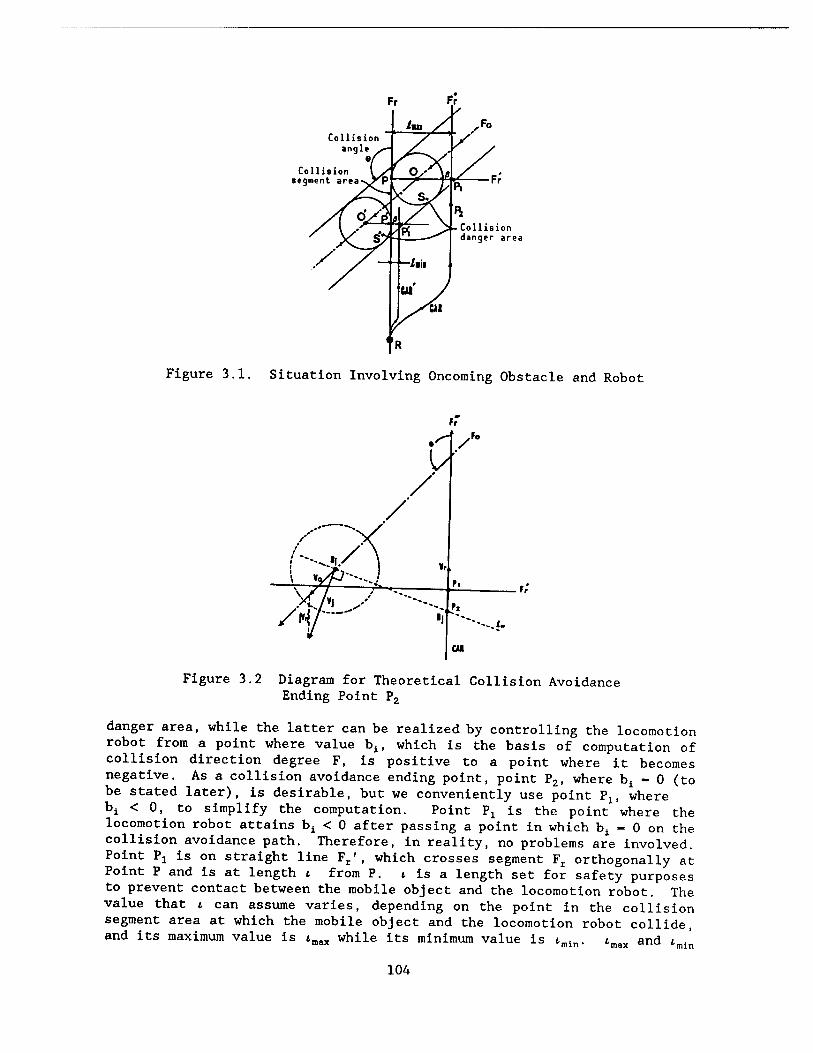
Collision angle

Collision segment area

Collision danger area

Figure 3.1. Situation Involving Oncoming Obstacle and Robot

Figure 3.2 Diagram for Theoretical Collision Avoidance Ending Point P2

danger area, while the latter can be realized by controlling the locomotion robot from a point where value bA, which is the basis of computation of collision direction degree F, is positive to a point where it becomes negative. As a collision avoidance ending point, point P2, where bL - 0 (to be stated later), is desirable, but we conveniently use point Plt where bi < 0, to simplify the computation. Point Px is the point where the locomotion robot attains bL < 0 after passing a point in which bt - 0 on the collision avoidance path. Therefore, in reality, no problems are involved. Point Px is on straight line Fr', which crosses segment Fr orthogonally at Point P and is at length i from P. t is a length set for safety purposes to prevent contact between the mobile object and the locomotion robot. The value that i can assume varies, depending on the point in the collision segment area at which the mobile object and the locomotion robot collide, and its maximum value is t_ax while its minimum value is i

min • and *min

104

correspond to the cases in which the mobile object collides with the locomotion robot at, respectively, point 0 and point 0'. Namely, «. is computed from the position of the mobile object at the time of collision, and its value is ß < i < 2(R0 + Rx) + ß. Here, R0 and Rx are the radii of, respectively, the locomotion robot and the mobile object, and ß is the length set for purposes of safety (Figure 3.1).

Let us next discuss collision avoidance path CAR.

A collision avoidance path is, as a principle, generated so that it may cross behind the mobile object (this is a principle of collision avoidance). This means assigning priority to the movement of the mobile object. The reason is as follows:

The mobile objects assumed in this paper include humans or locomotion robots and, in the collision avoidance action strategy, they are supposed to be at an intelligence level equal to, or higher than, that of the locomotion robot which is expected to devise solutions for various interference problems (e.g. , possibilities with other mobile objects) and unforeseen contingencies (e.g., appearance of a third mobile object) caused by the collision avoidance action of the locomotion robot. Therefore, the locomotion robot concerned must, when acting to avoid collision, not hinder the advance of the mobile object insofar as possible, and must be permitted a large measure of freedom in selecting actions. This policy is expected to have the subsidiary effect of simplifying the collision avoidance action of the locomotion robot concerned and making the structuring of a practical algorithm possible.

If an avoiding path cannot be formed, decelerate until the value of STATE 1 becomes SAFE. We will first examine the case in which the mobile object collides with the locomotion robot at point 0. The collision value is largest in this case. Here, consider straight line Fr" containing collision avoidance ending point T?1 and lying parallel to path Fr. Let the locomotion robot temporarily switch its path from Fr to Fr" to avoid collision with the mobile object. Part of the cosine curve is used for the transition from Fr to Fr" . The speed of the robot is controlled so that locomotion robot R may reach point ?x via path CAR when the mobile object arrives at point 0. At this time, point P2 can be determined as follows (Figure 3.2). Suppose that the locomotion robot is at position Rj at time j while moving along path CAR, and the mobile object is at position Oj. Use Vr and V0 as the moving vectors of the locomotion robot and the mobile object. The mobile object's vector relative to the locomotion robot is Vj. Find point P at which Vj vertically crosses the segment connecting Rj and 0j. Then, the value basic to the computation of collision direction degree F0 is bL < 0, and position Rj can be determined as point P2. After the completion of collision avoidance, the locomotion robot may or may not return from point ?1 to path Fr, depending on the purpose of the robot's movement. The case in which the mobile object collides with the locomotion robot at 0' corresponds with that in which the collision possibility takes the smallest value, and all that has to be done is to generate CAR' as a collision avoidance path.

105

We shall now observe cases with collision angles 0 of 90° > 6 > 0° and 360° > 6 270° (Figure 4). These are different from the above cases as follows: Collision avoidance ending point Px occurs when the mobile object is expected to collide with the. locomotion robot at point 0, and is at a distance R0 + Rx + ß from point 0 behind the mobile object on moving locus F0. Therefore, locomotion robot R is controlled so that it will reach point Px via path CAR when the mobile object arrives at point 0. This means that the recrossing of the newly-generated avoidance path CAR at points other than the proposed path F0 of the mobile object and point Px can be eliminated by setting the collision avoidance ending point Px behind the proceeding direction of the mobile object.

If the mobile object is to collide with the locomotion robot at point 0', point Px, determined by the same method as in the former case, becomes point Pj". But point Pi" is in the domain across segment Fr, opposite to collision avoidance path CAR that is generated when the mobile object will collide at point 0. If collision avoidance path CAR" is generated then, the locomotion robot tracks the mobile object. In this case, the locomotion robot follows the original path Fr and point Px' , at which a perpendicular from point P^' reaches segment Fr, can be used as the collision avoidance ending point, i.e., segment Fr" and segment Fr are identical. Then, distance between segments Fr and Fr" can have the value of 0 < i < (R0+Ri) + (RQ+R^/9) sinfl (Figure 4).

Collision

Collision segment area

i.,.

Collision danger area

Figure 4. Other Situations

Finally, we will discuss collision avoidance actions.

Here, the locomotion robot's position Rt' on avoidance path CAR at time t is determined as follows: This decision is made by considering position Rt of the locomotion robot when the absence of collision avoidance is assumed, drawing a segment parallel to segment O-Pj^ from point Rt, and computing, using the intersection of this segment and path CAR as Rt'. Therefore, collision avoidance by the locomotion robot can be controlled by gradually changing Rt to Rt'.

106

4. Collision Avoidance Test by Simulation

This chapter concerns the results of the simulation test we conducted to show an index of the suitability of this algorithm in regard to avoiding collisions with mobile objects. We will first illustrate the generation of avoidance paths, and then give an example of the case in which no avoidance paths are generated since it has been determined that the locomotion robot and the mobile object will not collide. Locomotion R£ is denoted with a contracted point, and mobile object 0it expanded proportionally to the contraction of the robot, is denoted with a double circle (Figure 5.1). Subscript i shows the INNER TIME (IT) of the robot. INNER TIME is time as defined by the robot itself. In this example, at IT - 0, mobile object 00 was discovered and measurement was initiated. In Figures 5.1 and 6.1, indication (a,b,c) on the right side (some, on the left side) of the proceeding direction Oi involves the evaluation of the danger of collision with the mobile object as measured by the movement information of the locomotion robot. a, b, and c represent, respectively, STATE 1, STATE 2, and STATE 3.

Figure 5.1 Example of Simulation (Generation of Collision Avoidance Path)

bi L M r lOr

1O-30

-10

20-

10

30-

Figure 5.2 Heuristic Evaluation for Figure 5.1

107

t- z D o u

II.M

lo~» **

—//—|

run i T i ji

II.M ■ ■ ■ .1.1 i i i i i i i i JJ l l i i i i i \U '*>'• \\r

DEGREE

Figure 5.3 Distribution for Figure 5.1

11

(a) (b)

Figure 6. (a) Typical Simplified Passages in Buildings (b) Example of Complicated Passages

4.1 Example of Cases Involving Generation of Collision Avoidance Paths

Here is an example of cases in which collision angle 6 satisfies the conditions of 90° > 9 > 0° and 360° > 9 > 270° (Figure 5.1) (an example of cases in which collision angle 9 satisfies the conditions of 6 - 0° and 270° > 9 > 90° was already shown in a KENKYU SOKUHO (RESEARCH NEWS FLASH)9).

The locomotion robot determines the collision possibilities while moving from R0 to R8, and generates collision avoidance path CAR at R8. The danger of collision of 08 at R8 is in the state of (MOST DANGEROUS, INTERESTING, and VERY VERY STRANGE). These three variables are the state variables mentioned in Chapter 1. STATE 1 is computed when the values of F and M at R0 to R8 continuously satisfy Equation (3), i.e., STATE 1 begins with DANGEROUS, becomes MORE DANGEROUS and changes to MOST DANGEROUS (Figure 5.1). When Equation (3) is satisfied, the collision direction degrees from R0 to R6 satisfy the condition F > 0 (Figure 5.2) and the collision wide angle degrees satisfy the condition M - 0 (Figure 5.2). Also, in evaluating the relative movement of the mobile object for the locomotion robot, the mobile object is judged to be headed for a collision (F > 0) and to be approaching the locomotion robot straightly, without lateral deflection (M - 0). Therefore, the robot separates collision avoidance path CAR, deciding that it will incur a collision if it moves along its original path. Then, from R8-R9 onward, the locomotion robot moves on the newly-generated collision

108

avoidance path CAR. At R9, 09 is in the state of (SAFE, INTERESTING, and VERY STRANGE), indicating that collision has been avoided. The subsequent state of the locomotion robot is maintained at SAFE and INTERESTING in, respectively, STATE 1 and STATE 2. Also, STATE 3 changes from VERY STRANGE to STRANGE and finally to NONSENSE, and thus the state becomes increasingly safe. This shift from danger to safety can also be understood from the change of the values of bi, F, and M (Figure 5.2). The change of the bL

value indicates that the locomotion robot has avoided the mobile object from bj > 0 to bt < 0 for its movement from R16 to R17 and that, furthermore, it has shifted to a collision-free state. As can be understood from the movement from R8 to R9 in Figure 5.1, the temporary increase of the bi value at R9 and R10 is due to the fact that the locomotion robot and the mobile object suddenly approached for a while. This sudden approach is clear from the change of the rate of decrease of approach degree L (Figure 5.2). Its effect is apparent in the value for F, namely, the variation of the F value in the vicinity of R10. At this time, the state of the locomotion robot may be considered to have become temporarily dangerous through the increase of F, but no problems exist since STATE 1 is already SAFE. Later, with F decreasing and M increasing, the locomotion robot shifted to a state of greater safety. Movement angle record D in this simulation is shown in Figure 5.3. At the absolute azimuth DGR - 0, the locomotion robot discovered the mobile object and no change occurred in the value of DGR for the movement angle was high and positive. By this value, the state variable of the mobile object, STATE 3, became VERY VERY STRANGE. The movement from R0 to R9 in Figure 5.1 corresponds to this. At DGR = 10-80, the count was relatively even. The movement from R10 to R16 corresponds to this. At DGR = 120, the count showed a negative value. This means that bL became negative for the movement at R16~R17.

5. Discussion of Case With Limited Space for Avoidance Actions

In this chapter, the problem of a locomotion robot generating a path for avoiding collision with a mobile object will be discussed with respect to cases involving limited space for avoidance actions, specifically cases in which collision avoidance occurs in passages in buildings. As limited space, we will deal with an expanded wall section in a like manner as when we contracted a locomotion robot into a point and expanded a mobile object.

5.1 Limitation of Movement Space

The forms of passages often encountered by locomotion robots within the interiors of buildings are straight, L-shaped, T-shaped, and cross-shaped passages, which may be referred to, respectively, as I-shape, L-shape, T-shape, and +-shape. It is necessary to study the problem of collision avoidance for these four types of limited space11 (Figure 6(a)). A more realistic passage form (Figure 6(b)) is a stretch of I-shaped passages with different widths. It is assumed that the locomotion robot has full knowledge of the structure of the working space through which it moves, i.e., such matters as the presence of walls and their size, and that the space contains no desks, chairs or other fixed objects independent of the walls.

109

5.2 Example of Simulation in Limited Moving Space

The following are the results of our simulation of collision avoidance in a +-shaped passage. This +-shaped passage is composed of walls HlP H2, H3, and H<, (Figure 7). Suppose that a locomotion robot appears from below, a mobile object appears from the left, and it is known that they will collide at the position R0 and 00. The locomotion robot immediately generates collision avoidance path CAR by the method proposed in this paper and acts to avoid collision. This example shows that the locomotion robot acted in accordance with the principle of collision avoidance by crossing behind the mobile object.

Figure 7. Example of Simulation in Limited Space

6. System Target and Its Composition

This system is composed of a host computer linked to several locomotion robots by radio (Figure 8). The locomotion robots are each composed of an educational robot system HER02000 (Heathkit product) equipped with a CCD camera visual system.12 The visual system is a stereo visual device using two CCD camera13 or a Canon 3D visual sensor using a CCD camera.1* HER02000 has as an existing sensor an ultrasonic sensor that can detect obstacles lying within a circular perimeter with a radius of about 3 m. The ultimate target when searching for mobile objects involves the sensor fusion of the visual system and the ultrasonic sensor. The robot has a local map for the small domain of the time of movement and can, using the map to identify its position, discover an obstacle and determine whether the obstacle is moving. The local map is small, using information from the global map provided on the host computer.

The robot is linked to the host computer and can use information stored in the memory or can update information. A person can exchange information with the locomotion robot via the window system of the host computer. If, for instance, a person gives the robot an order to move from one point in the building to another, the robot can move to the destination while automatically avoiding collision against a fixed or mobile obstacle that exists in its locomotion environment.

110

Each of the robots linked to the host computer can move along a noncollision path planned by the host computer. There is no problem involving collisions between robots for which noncollision paths have been planned. The host computer used is the SUN 3/50. It uses UNIX 4.2 BSD for OS, and COMMON- LISP, K-PR0L0G, and C language. The systems to be developed by the host computer are as follows:

Global map management system Noncollision path generating system Own position estimating system (on global map) Unknown domain searching system Mobile obstacle management system Management system for several robots CG-using collision avoidance simulation system

Developed system and computer

Visual system

^ Ticture proc- essing systtrr

Central pro

169 K * ft. 3E Ultra sonic system

HERO system

V. (8888)

r Small

system

Figure 8. System Composition

To develop systems, HU68K of X68000 and C language are used for HERO2000's picture processing system and the central control system, and B language on PC 98's MS-DOS is used for the HER02000's drive system. The B language referred to here is the C-like BASIC filter program developed by the authors' research group. The systems to be developed on the robot are as follows:

OS for robot use (MCMS) Local map management system Mobile object monitoring system Collision avoidance system Own position estimating system (on local map) Visual control and processing system Robot traffic rule applying system Escape system

111

7. Basic Test Using Actual System

The authors conducted a collision avoidance basic test using a small system to see if the proposed collision avoidance algorithm could be realized by an actual system.

The small system used is shown in the dotted-line area in Figure 8. In this test, we used an ultrasonic sensor to detect mobile objects.

The concept of the test is as follows:

The locomotion robot, moving at a constant speed through a building passage that has no fixed obstacles other than walls, uses our proposed method to avoid colliding with a single mobile object approaching at a constant speed.

The algorithm for avoidance collision has been developed by the B language on the PC98 and is used by being downloaded to the robot's memory.

The mobile object is a person. For the space in which the robot moves, typical simplified building passages have been conveniently constructed, using plywood, 10 mm in thickness, as walls (Figures 9 to 11).

Figures 9, 10, and 11 show collision avoidance being tested on, respectively, an I-shaped, A T-shaped, and a +-shaped passage.

The robot confirms its present position on the passage and the presence of surrounding walls from local map information, discovers the mobile object and acts to avoid colliding with the oncoming mobile object. The local map is composed of a set of information comprising the passage and the intersection lying ahead.

In this test, 2.4 m was always used as the passage width.

The experiment in Figure 9 illustrates the case with a 0° collision angle, i.e., the mobile object approaches the robot from behind. The initial positions of the two are 1.2 m apart. The robot discovers the mobile object as it moves, then predicts collision, estimates the position of collision at 1.2 m from the initial position of the robot and avoids collision accordingly.

The experiment in Figure 10 illustrates the case with a 90° collision angle. The collision point was 2.3 m from the initial position of the robot and 1.9 m from the mobile object.

The extension cables behind the robot comprise a charging 2p cable and an RS232C cable for collecting test data. Therefore, these cables do not impair the autonomy of the robot.

112

Figure 11. «-Shaped Passage

113

8. Conclusion

In this paper, we have proposed several methods to enable a locomotion robot to avoid collision with an oncoming mobile object, and have described a basic test involving collision avoidance by an actual system using these methods. We first proposed collision possibilities, and then proposed how to generate collision avoidance paths. We discussed a method to avert collisions between the robots themselves, using building passages as an example. We also studied, by simulation, the effectiveness of the collision avoidance methods proposed in this paper. Finally, we conducted a basic test on collision avoidance on a small experimental system using the educational robot HER02000. In this test, both the robot and a person, as the mobile object, moved by steps, and we showed examples of a collision avoidance test in simplified building passages using an actual system. Tasks for the future include the realization of smooth collision avoidance actions of the robot, the realization of a collision avoidance robot using the sensor fusion of an ultrasonic system and a visual system, and the clarification of the case in which mobile objects and fixed objects coexist, the case in which several mobile objects exist, the case in which the mobile object itself acts to avoid collision and the problem of simultaneous collision avoidance.

References

1. Kakikura, "Trends of Autonomous Locomotion Robot Elemental Technology: Technology To Make Autonomous Locomotion Robots Intelligent (1) Action Planning (Commentary)," JAPAN ROBOTIC SOCIETY JOURNAL, Vol 5 No 5, 1987, pp 398-402.

2. Kakikura, Mishima, and Osada, "Storage Composition of Intelligent Robot and Its Application to Rule Searching," SOCIETY FOR INSTRUMENTATION AUTOMATIC CONTROL JOURNAL OF PAPERS, Vol 9 No 1, 1971, pp 45-50.

3. Fujii, Morita, and Yanaida, "On How To Plan Path Searching of Intelligent Robot," SYSTEM AND CONTROL, Vol 15 No 11, 1971, pp 68-75.

4. S. Tachi and K. Komoriya, "Guide Dog Robot," Proc. Second Int. Symp. of Robotics Research, MIT Press, 1984, p 333.

5. H.P. Moravec, "Obstacle Avoidance and Navigation in the Real World by a Seeing Robot Rover," Stanford Univ. Tech. Rep. AIM-340, 1984, p 1.

6. S. Tachi, K. Komoriya, K. Tanie, T. Ohno, and M. Abe, "Guide Dog Robot-Feasibility Experiments With MEL-DOG MARK," Proc. 11th Int. Symp. on Industrial Robots, 1981, p 95.

7. E. Freund and H. Hoyer, "Pathfinding in Multi-Robot Systems-Solution and Applications," IEEE Proc. Int. Con. on Robotics and Automation, 1986, pp 103-111.

114

8. Takeno and Kakikura, "Basic Studies Concerning Collision Avoidance of Locomotion Robots--Report 1: Decision of Possibilities of Collision, Generation of Avoiding Paths and Accommodation in Limited Moving Space," 3d Intelligent Locomotion Robots Symposium, No 7, June 1986, pp 37-42.

9. Ibid. , "On the Problem of Locomotion Robot Avoiding Collision Against Mobile Obstacle (Research News Flash)," JAPAN ROBOTIC SOCIETY JOURNAL, Vol 4 No 5, October 1986, pp 33-37.

10. Ibid., "Basic Studies Concerning Collision Avoidance of Locomotion Robots--Part 4: A Method To Generate Collision Avoiding Paths in Collision Segment Area," 29th Automatic Control Federation Lecture Meeting 2015, November 1986, pp 299-300.

11. Ibid., "Basic Studies Concerning Collision Avoidance of Locomotion Robots--Report 1: A Method To Generate Paths for Avoiding Collision Against Mobile Obstacles," 4th Robot Engineering Subcommittee Seminar, Society for Instrumentation Automatic Control, RS-88-3, March 1988, pp 19-28.

12. Higuchi, Yatsuyama, Takeno, et al., "Basic Studies Concerning Collision Avoidance of Locomotion Robots--Part 8: A Proposal on Collision Avoiding Robot," 5th Japan Robotic Society Scientific Lecture Meeting, 1404, 1987, pp 121-122.

13. Yatsuyama and Takeno, "For Collision Avoidance Study--Part 2: On an Experiment," 34th Information Processing Society National Convention, 6D-3, 1987.

14. Mizuguchi, Takeno, et al., "Basic Studies Concerning Visual System for Collision Avoidance--Part 3: A Method To Plan Mobile Obstacles by Means of 3D Visual Sensor," 5th Japan Robotic Society Scientific Lecture Meeting, 1405, 1987, pp 123-124.

115

Collision Avoidance in Locomotion Robotic Systems

43064062 Tokyo 4TH INTELLIGENT ROBOTS SYMPOSIUM PAPERS in Japanese 13/14 Jun 88 No 204 pp 85-90

[Article by Mamoru Saito, Osaka City Industrial Research Institute and Toshihiro Tsumura, University of Osaka Prefecture]

[Text] 1. Introduction

A vast amount of information and computation concerning all vehicles has been necessary to effectively implement operation control for vehicles used in systems, including the new transportation system and the factory unmanned conveyance system. In striving to achieve intelligent locomotion robots, the tendency in recent years has been to prefer using the flexible and extendable control system of the autonomous dispersion type as a control system for these locomotion robot systems. There, only the limited information between nearby locomotion robots is used when determining control inputs. It is important, therefore, to maintain the consistency of the whole system by coordinating the locomotion robots while making the most of the independence of individual robots.

This study concerns collision avoidance in the locomotion robot system as just one of the problems involved.

A number of studies on collision avoidance have been conducted involving industrial robots in the past. In these studies, the method has consisted of first modeling work space according to visual information by the ultrasonic sensor, the CCD camera or some other means, and then evaluating the relative relationship to the obstacle.

Proposals made in them include:

(1) Method of defining the heuristic function and generating collision avoidance paths (2) Method of defining the potential function and avoiding collision while correcting the speed vector

Many of the studies are cases handling the problem of robots as individuals, and none show a method effective for a dispersive system composed of several robots.

116

The authors previously proposed an algorithm to avert collision between locomotion robots using a heuristic method, and proved its effectiveness by simulation using an equivalent two-wheeled model for the robot dynamics.

There, we stated the case of controlling the traveling azimuth, using the same speed for all robots, as a method of collision avoidance. However, in this article, we will report the case of controlling the speed, using the same traveling azimuth for all robots.

The algorithm used here is basically the same as that previously proposed, and its procedure is:

• Each of the nearby robots gains information regarding the position and speed of the other by vision or communication.

• Each evaluates the relative relationship and predicts collision.

• If collision is predicted, a vector for suggested speed aimed at avoidance is derived according to the rule of coordination.

• Avoidance is effected as real-time processing by causing the robots to follow it.

2. Problem Setting

As indicated in Figure 1, n-number of robots moving to their destinations by their autonomous guidance functions on a plane without obstacles is assumed as a model for the locomotion robot system.

Figure 1. Conceptual Diagram of Locomotion Robot System

Each robot is supposed to have

• Inherent domain

This is a domain with a radius of r± which the robot occupies. It is determined according to the size and shape of the robot.

117

• Detecting domain

This is a domain with a radius of R^ for recognizing the presence of the other robot (position, speed, etc.)- It is determined according to the size of ri and the moving speed.

In this article, our discussion presupposes that all robots have the same

3. Predicting Collision

Each robot evaluates the relative relationship between it and another robot which has entered its detecting domain from information regarding the position and speed of the other robot.

Suppose that, in Figure 1, at time k, the positions of robots are xL(k) and Xj(k) and their speeds are x^k) and Xj(k). Then, x^k), the relative position vector, and jq^k), the relative speed vector, of robot j , as viewed from robot i, are

rX|j (k)-X)(k)- xi(k) (1) Lxi) (k)-xj (k)- xi(k)

Assuming that the robots move at constant speeds, L^t), the predicted distance function time t from now, is defined as follows:

Lij(t) • I xiJ(k)t+xi](k) I' (2)

At this time, the state between these robots can be determined by the differential value of LXj(t) at the current time (t - 0). Namely, if the value is negative their distance decreases, and if it is positive the distance increases.

Therefore, the conditions under which their collision (each invading the inherent domain of the other) is predicted are:

a$Lij(o)<o (3)

tLij (t) ] «in < Crt ♦ ri)* (4)

4. Derivation of Suggested Speed Vectors

If robots i and j are in the state of possible ^collision (conditions in equations (3) and (4)), find the solutions for x^j.k) and Xj(j,k), with their respective corrected speed vectors satisfying equation (5), to avoid the collision.

[L ij(t) ] iin = ( rt ♦ r j)» /^\

Considering robot i_first, this can be obtained by replacing speed vector xA(k) with variable xx(j,k) in equation (5).

118

So, draw up

■i;(k)= xi (j,k)= (xj.x,) xij(k) - (P,.P,) ,xj(k)= (n.»,) rij = rj + r. (6)

(here plt p2, vx, v2, and rid are known numbers from the preceding process) and substitute it for equation (5).

At this time, equation (5) can be consolidated into the following quadratic equation:

y'Ay = o (7)

■a,0 O-i a,= rtj •

Here,

0<x,0 0 0 0-1 cc,= r,,«- (pt« +p,i )

[vt -| r Pi«t*Ptit-(pi»t*p»ii) -i ?t = -Pi«t*Piii-(p,»t-P»T,)

Therefore, equation (7) can be solved as

VST y» = ±V-«i vt (8)

The geometrical meaning of equation (8) is that it represents the two straight lines shown in Figure 2. This is a set of solutions for corrected speed vector xi(j,k) in which robot j avoids robot i relatively by right or left and it cannot, as it is, be determined uniquely.

So, set the following constraining condition for xi(j,k), considering the case in which a robot moved on a straight path toward its destination:

*i/x2 - cL (9)

Two solutions can be found from equations (8) and (9) (Figure 2). So, to use only one solution:

(1) Avoidance by left (Solution xf(j ,k) determined by Ja-^y^^ = J-o^zYz and equation (9), is used as the suggested speed vector d^j,k)

(2) Use of the robot's limiting speed Vmax as the suggested speed vector if the solution of dA(j ,k) exceeds Vnax is set as a rule of coordination between the robots.

119

■ -i-' ' r »fc • t I /

i

Figure 2. Relationship Between Robots i and j

Here, due to the setting of (2), the robot may stop and retrogress, depending upon the problems present. However, this does not occur if the difference in speed or inherent domain between the robots is small.

By now, the suggested speed vector dA(j ,k) for robots i and j has been determined. Robot i conducts similar processing for other robots that are in its detecting domain, and d*(k) (MAX(| dA(j ,k) -x^k) ||)), the suggested speed vector in which the absolute value of the difference from the present speed is the greatest, is used as the final suggested speed vector D^k).

/x7(i(), x.(k)/

d .(J.k>'X?<j,k>

i*i*i

k -k + 1

D <k>- d~(k>

JL Strvo &

Robot dynaaies

d <j,k)«x <k>

d ^k) : «ix ( II dt(j.k)-x t<k> II >

Figure 4. Collision Avoidance Algorithm for Locomotion Robots

The above collision avoidance procedure is consolidated in Figure 4. same procedure is used for robot j.

The

120

5. Simulation

(1) Design of Control System

Here, we shall design a method using LQ control as a robot follow-up system for the suggested speed vectors obtained by the foregoing procedure.

First,

ms + cs = au (10)

is assumed as the robot dynamics. s is the robot's position and u is its control input. We also used

c (coefficient of viscous friction) x m (mass) =0.2 a (gain constant) x m (mass) =0.3

If state variable x = ('s s)T and control input ü = u are used to formulate a speed control problem involving the robots, the following state equation expressed by discrete time can be derived from equation (10):

rx(lel)-Ao x (k) +B„ ü (k) Ly(k)-Cx(k)

(ID

Here,

r ' 4.38X10'

A, -

L o 9.90X10

C = [ 1 0 ]

XIU -1 r3.74X10~-i

B.- XIO-'J L1.49X,0-«J

To enable the robot to follow target value r of the suggested speed, it is necessary to put

re(k)-r -y(k) u(k)-ü(k*l)-ü(k) M (k)-x(k*l)-x(k)

(12)

and compose the next extended system:

U (k*0 3£

A» 0

-C I

?(k)

«(k) +

r Bo

o. l(k)

«(k) - [o »] (k]

(k)

'

(13)

Since this extended system is attainable, üopt(k), the optimum input with

JC»] = ,1 U(k)«*q n(.k)>) k=0

(14)

as a minimum, can be obtained as an evaluation function by the next equation:

121

ü.,i(k) * KxOO+KtScCD+const. 1*0

(15)

It is known that feedback gains here, K and KI( can be given from the solution of the Riccati algebraic equation.

In our simulation, therefore, we assume 0.1 to be the weight coefficient q and use

K - [-4.4 x 101 - 1.61 x 101], Kr - 2.78

computed on this basis.

T0M2

IM

(»-0 Loci of locomotion robots

«ft"

MSB Tllf(SK)

..1 "t>,

-J.«

l7S I. ii.BM a« ) TIICIMC)

• ■ / ft s

:

......

lb ^

-i.«

(a-2) Response to suggested speed

Figure 5. Avoidance of Collision Between Two Robots (Case without speed limitations)

122

IM

IM

A robot 2

IrfjV' * m m i .>»:£? jifc<ai33al al23 robot 1

(a-1) Loci of locomotion robots

robot!

iCEixs:;;::icci:;s;^-a332332B robot l

(b-1) Loci of locomotion robots

robot 1

IM

(c-l) Loci of locomotion robots

(rr A"

i.a \ 4; h

■l.a ::s:

I. (We) 1.«

m ft ~x. 1 ■

it.« TltElHC)

(t-2) Response to suggested speed

'IT»

^ ,.*.'.

::Tn tj^. a. a

'Oi

(•uket) l.n

ii. en TllCUeO

■M •Siil

^ :*i

L ■•■

....:

io.a» Tllt(WC)

(b-2) Response to suggested speed

*s* /*•

i.a

-i.a

<*.

t.

i.a" ii.aa TIIC(MC)

* t.B "^

-i.a

it.as TIIC<KC|

(c-2> Response to suggested speed

Figure 6. Avoidance of Collision Between Robots (Case in which speed is limited)

123

(2) Results of Simulation

Here, as basic collision avoidance, we studied a case using two robots (Figures 5 and 6) and one using four robots (Figure 7).

rebotj

»tori

IM

BEEEEEECEKUCO robot 3

IM (a) Case in which avoidance is

possible

(b) Case in which avoidance is impossible

Figure 7. Collision Avoidance Among Four Robots

The simulation conditions are shown in Table 1. However, in the cases shown in Figure 7, 0.5 m/sec and 1 m/sec were used for all robots as, respectively, the set speed || x^O) j| and limiting speed Vmax.

Table 1. Simulation Conditions

-—________ robot 1 robot 2

M«0 1

R.«0 S

II xi (0)11 OVsee) 0.5 | 0.25

v.t. (m/sec) 1

Figure 5 concerns a case of collision avoidance in which the above-mentioned rule of coordination (2) was not set (i.e., without a robot limiting speed). It can be seen that the control systems of the robots cannot follow the suggested speed sufficiently, whereas, in a similar case involving rule of coordination (2) (Figure 6 (a-1)), collision is safely avoided.

As can be presumed from the three cases shown in Figure 6, it is believed that collision avoidance between two robots is feasible as long as the moving paths of the robots do not overlap.

Regarding the problem in which three or more robots are involved, this algorithm is applicable if, as indicated in Figure 8, the conditions under

124

which all robots can pass simultaneously within the area enclosed by the crossing of their moving paths are satisfied.

robot i

Figure 8. Conditions of Moving Paths Making Collision Avoidance Possible

Figure 7 is a case involving four robots, mentioned conditions are not satisfied.

The robots stop if the above-

Conclusion

We have proposed an algorithm by which, in a dispersive system composed of more than one locomotion robot and based on the assumption that each robot is moving along a straight path toward its destination, the robots control speed according to the prediction of their mutual relative relationship, thereby avoiding collisions.

We have shown here that avoiding collision according to different situations is possible by effecting speed control, with the speeds limited according to a rule of coordination between the robots. We have also confirmed the effectiveness of this algorithm by designing a robot followup system using LQ control measures and verifying it by simulation. In the future we will also study designing locomotion robot operation and controlling their orbits.

References

1. Yoshikawa, et al., "Distributed Control of Vehicle Group on Ring Route," SYSTEM AND CONTROL, Vol 24 No 10, 1980, pp 690-698.

2. 0. Khatib, "Real-Time Obstacle Avoidance for Manipulators and Mobile Robots," Int. Conf. on Robotics and Automation IEEE, 1985, pp 500-505.

3. E. Freund and H. Hover, "Path Finding in Multi-Robot Systems," Ibid 1986, pp 103-111.

Saito and Doi, "Avoidance of Collision Between Robots," 1st Symposium of Vehicle Automation Technical Research Association, February 1988.

125

Search Capability of Locomotion Robot in Unknown Environment

43064062 Tokyo 4TH INTELLIGENT ROBOTS SYMPOSIUM PAPERS in Japanese 13/14 Jun 88 No 205 pp 91-96

[Article by Junichi Eijima, University of Electrocommunications; Takashi Takeuchi, NTT; and Shinichi Aburada, Tsukuba University: "How To Search for Unknown Environments by Means of Locomotion Robot--Simulation Using Sensor

Models"]

[Text] 1. Introduction

A locomotion robot normally moves with the help of an existing map but, if it could operate a location not on a map or in one with only an unreliable map, more useful activities could be expected of it. The purpose of this study is to establish a basic format for the operation of robots in such unknown places.

Studies already announced with similar purposes include Hirose, et al.'s map producing visual system,1 Tazumi, et al.'s locomotion robot observational operation planning system,2 Ichikawa, et al.'s study concerning map revising,3 and Chatila, et al.'s system taking sensor system errors into consideration.*

Here, let us consider the search for unknown environments to involve releasing a locomotion robot into a medium-size room in order to search the interior of the room and, after an appropriate period, causing it to prepare a map of the room and the obstacles in it. The robot basically prepares the map by observing the periphery with an environmental sensor, preparing and enlarging a map, forming a movement plan and repeating movement. Specifically, this involves the following problems: 1) determining its next destination and the attitude to be assumed there, 2) determining its path of movement, 3) determining the completion of its search, 4) movement planning and the form of expression to be used to determine the completion, and 5) preparing a map in which errors attending movement and errors of the sensor system are taken into account.

The authors previously proposed a search method (corresponding to 1), 3) and 4) above) using two types of map information--grid expression and vector expression--and indicated that, in an ideal case without sensor errors, it

126

would be possible for the robot to search, sensing unknown environments on a real-time basis.5

In this study, to cope with accidental errors occurring to internal and external sensor systems in the real world, we have corrected errors of robot positions by fusing errors in sensor systems and have extended our previously proposed method so that more reliable maps can be composed We have also evaluated the effectiveness and realizability of this method by simulation using models of sensors in which errors occur.

2. Problem Setting

Let us first examine the unknown environment conditions to be searched by a locomotion robot and the modeling of internal and external sensors containing realistic errors. We will assume a wheel-shaped locomotion robot with a range finder as an external sensor, and as an internal sensor, a travel recorder to estimate the current position of the robot from the per- unit-time rotation of the driving wheel.

2.1. Environmental Conditions

We have studied the following environments:

(1) In a building with a nearly level floor and of a certain size (about 20 m2), the robot can move freely if no obstacles exist.

(2) There is more than one room in the environment and the rooms contain furniture and other obstacles, but no mobile objects are present except for the robot.

(3) The shape of the silhouette of an obstacle projected on the floor can be approximated to a polygon with a side of at least 20 cm.

(4) The shape of the locomotion robot can be approximated by a circle with radius rb (= 40 cm).

2.2 Model of Internal Sensor

In the robot "Yamabiko No 9," which the authors developed, accidental errors occurred when tracking (dead-reckoning) the position of the robot by the internal sensor were within 1-2 percent of the moving distance for position and ±1° for attitude. Therefore, in the simulation model of an internal sensor with errors, the robot positional error must be expressed by a two- dimensional normal distribution with a standard deviation of 2 percent of the moving distance. As for the robot attitudinal error, it must be absorbed by this positional error, as well as by the errors of the external sensor which will be described next.

2.3 Model of External Sensor

The robot must be able to measure its distance to an obstacle located within a certain distance, from rmin (= 50 cm) to rmax (= 400 cm), in any direction,

127

by the external sensor when it remains at a certain position in the environment. By processing the measured distance data, one can detect the polygonal domain formed by projecting onto the floor the space in which the robot can move freely within the range of observation (free space). It is assumed that, in reality, a polygon can be obtained which is composed of defined boundaries and edges resulting from the inability to observe due to being behind obstacles, etc., or being beyond the range of observation (free space). It is assumed that, in reality, a polygon can be obtained which is composed of defined boundaries and edges resulting from the inability to observe due to being behind obstacles, etc., or being beyond the range of observation (provisional boundaries) (Figure 1). Such a ranger finder can be realized by, for example, turning a TV camera ±180°.

Object

Solid line: Defined boundary

Dotted line: Provisional boundary

Figure 1. Measuring Range of Range Sensor (External Sensor)

A range finder incorporating errors has been modeled as follows (Figure 2): First, a normal random number with a standard deviation of 1 degree is assigned to each apex of the polygon which exhibits ideal, errorless free space and is obtained from the environmental data given in advance in the line-of-sight direction of the apex (Figure 2(2)). Then, a normal random number with a standard deviation of 6 cm is given in the depth direction of the camera's line of sight to points, about 0.2 degree apart, on the sides of the defined boundary of this polygon (Figure 2(3)). Each point is regarded as a mass point, its 0~2-order moment and principal axis of inertia are obtained, and its inclination is used for the defined boundary (Figure 2(4)). However, a defined boundary with less than 5 degrees as the angle difference, estimated on the basis of the beginning and end points is regarded as a provisional boundary since its position cannot be obtained with high precision, even though it has been detected in the picture as an edge.

The above values of standard deviation, etc., were determined from our test experience using a visual sensor with a CCD camera.

3. Method of Map Expression

When a robot operates in unknown environments, no maps are available, so it must prepare one for itself. In this case, the map must be composed on a real-time basis from definite observed data. Therefore, it is advisable that an expression be used that is more specific, material and succinct. Here, two types of maps with two-dimensional expressions are used together. These maps are referred to as vector and grid maps.

128

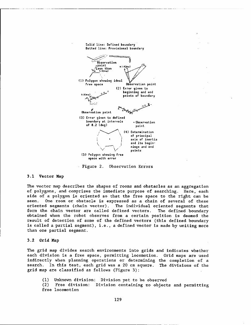
Solid line: Defined boundary Dotted line: Provisional boundary

'Observation •point

/Less than S.OUei)

(1) Polygon showing ideal free space Observation point

(2) Error given to beginning and end

o.iKctl ^ points of boundary

Observation point

(3) Error given to defined boundary at intervals of 8.2 (deg)

• Observation point

V (5) Polygon showing free

space with error

(4) Determination of principal axis of inertia and its begin- nings and end points

Figure 2. Observation Errors

3.1 Vector Map

The vector map describes the shapes of rooms and obstacles as an aggregation of polygons, and comprises the immediate purpose of searching. Here, each side of a polygon is oriented so that the free space to the right can be seen. One room or obstacle is expressed as a chain of several of these oriented segments (chain vector). The individual oriented segments that form the chain vector are called defined vectors. The defined boundary obtained when the robot observes from a certain position is deemed the result of detection of some of the defined vectors (this defined boundary is called a partial segment), i.e., a defined vector is made by uniting more than one partial segment.

3.2 Grid Map

The grid map divides search environments into grids and indicates whether each division is a free space, permitting locomotion. Grid maps are used indirectly when planning operations or determining the completion of a search. In this test, each grid was a 20 cm square. The divisions of the grid map are classified as follows (Figure 3):

(1) Unknown division: Division yet to be observed (2) Free division: Division containing no objects and permitting free locomotion

129

(3) Boundary division: Division crossed by a defined boundary (4) Occupied division: Division in which locomotion and observation are impossible

D Unknown division E5 Free division

0 Boundary division

■ Occupied division

Figure 3. Classification of Divisions

An unknown division is reclassified as either a free division, a boundary division or an occupied dot elimination as searching progresses.

4. Searching Method

We shall now discuss the basic concept of the searching method, the method to prepare and extend a more accurate environmental map from erroneous sensor data and the method to correct deviation in the position of the robot, taking advantage of information from the environmental map prepared by the robot.

4.1 Basic Concept

Previously, we proposed a love-at-first-glace method aä a way of planning the operation of a locomotion robot which would enable the efficient searching of an unknown environment to be accomplished.

In this method, the locomotion robot released in an unknown domain first observes the periphery by an environmental sensor, notes the longest of the chain vectors in the local vector map, and selects, as the next locomotion point, a position from which the end point and its vicinity can be observed so that the end point may be gradually extended. The robot observes from varied positions and uses the data gained to extend the vector and grid maps. In the vector map, new chain vectors are added and chain vectors already detected are extended. In the grid map, on the other hand, the unknown division is reclassified into a free division or a boundary division. When extending the map, errors in sensor data are taken into consideration. This will be described in the next section.

When searching progresses and the chain vector being pursued closes to form a polygon, the unknown division on the left side of the chain vector is reclassified into an occupied division. Then, the same principle of locomotion is applied to all chain vectors yet to be closed. If there are unknown divisions on the grid map when no chain vectors remain to be closed, the point from which the nearest unknown division can be seen is selected as the next locomotion point.

When all chain vectors detected are closed and no unknown divisions remain on the grid map, searching is completed and the environmental map is ready.

130

4.2 Extending of Maps

We will now discuss the extending of the vector and grid maps.

4.2.1 Data Composition in Vector Map

In the vector map, all partial segment data (local vector map) obtained on each occasion of observation are preserved, and the aggregation of component partial segments is coordinated to each defined vector. Therefore, elaborate correction of the vector map becomes possible by enabling the data medium on partial segments observed at each corrected position of the robot to correct defined vectors containing these data and chain vectors each time the position of the robot is corrected.

The vector map can be obtained by first computing each defined vector from the partial segment and then causing the apices of the connected defined vectors in the chain vectors to agree, thereby guaranteeing their connnectivity.

When partial segments are added, the moment and inclination of defined vectors are computed again, using the moment of the partial segments composing them. Therefore, the positional information of partial segments must include not only information on their beginning and end points and inclination, but also information on their 0-2-order moment and the positional error of their beginning and end points (= predicted positional error of robot + observation error) and information to show whether the beginning and end points are apices denoting objects, etc., or whether they are mere terminal points. As for each moment of a defined vector, the weighted mean by the inverse of the positional error (standard deviation) of the robot at the time of observation is used for each moment of each partial segment composing the vector.6 If, for instance, three partial segments: llt 12, and 13, are united as a defined vector, each moment Mid (i,j - 0-2) is computed as follows:

■ li Ja ifi2.i/0zti3. ,/a 3 Mu= —; ;, ■ . , . (Equation 1)

Here, ml^, m2ij, ntf^ (i,j = 0-2) comprise the moment of each segment around the origin in the coordinate system common to these segments, and ax, a

2, and a3 are the positional errors (standard deviation) of the robot at the time of observation of each segment.

The beginning point (end point) of a defined vector is obtained as follows:

(1) If the partial segment contains beginning points (end points) denoting apices, use the weighted mean by the inverse of the square (dispersion) of the positional error for these points (probable maximum value). For the positional error at that time, use the smallest of the positional errors at the beginning (end) points of the partial segments expressing apices.

131

(2) If this is not the case, use the point farthest from the center of gravity of the defined vector. The positional error at that point is used as the positional error of this defined vector.

Finally, for two defined vectors connected in a chain vector, the weighted mean by the inverse of the square of positional errors at the end point of one and the beginning point of the other is used as their intersection, thereby guaranteeing their connectivity.

4.2.2 Extending Vector Map

The method used to add information from the local vector map, a result of our recent observation, to the vector map prepared by consolidating the results of our past observations, can be divided into the process uniting the defined vectors in the vector map and the partial segments on the local vector map and the process connecting them.

The conditions for the overlapping of a defined vector and a partial segment are as follows (Figure 4):

Segment

diff.lh

Condition® : diff.lh ai TjM

Condition (?) : d',5,* * TH2

Figure 4. Conditions for Uniting Segments

(1) The angle difference between the two segments is less than a certain threshold value, TH1.

(2) A perpendicular from any of the four beginning and end points of the two segments can be drawn from either segment to the other, and the length of this perpendicular is less than threshold value TH2.

(In the test, we used TH1 - 30.0 [deg], TH2 - 50 [cm].)

The conditions for connecting the beginning (end) point of a defined vector and the end (beginning) point of a partial segment are as follows:

(1) Both points are detected as apices of obstacles, etc.

(2) The distance between the two points is less than certain constant multiplied by the value C of the larger of the positional errors at these two points.

132

A positional error is a standard deviation in normal distribution. Therefore, if C - 1, 2, and 3, the two points, if they actually are equivalent, can be connected by the probabilities of, respectively, approximate 68, 95, and 100 percent. However, if C is too large, it follows that two points that, in reality, are not equivalent are connected. Therefore, in this case we used C = 2.0.

4.2.3 Extending Grid Map

At the beginning of a search, all divisions of the grid map are unknown divisions. In each observation, appropriate unknown divisions in the vicinity are changed into free divisions or boundary divisions (divisions containing chain vectors). In addition, when the chain vectors close on the vector map, the unknown divisions contained in the closed domain surrounded by these vectors become occupied divisions.

In our recent test, we used divisions that were as large as 20 cm2. Therefore, it is believed that errors in the internal and external sensor systems of or about the order state in Chapter 2 can be absorbed almost completely.

4.3 Correction of Robot Position

During searching, deviations in the current position of the locomotion robot are detected and,if necessary, corrected, using vector maps prepared previously. This is done by noting the apices of walls and obstacles as a characteristic of an environment, and is divided into correcting the current position of the robot and correcting past positions.

4.3.1 Correction of Robot's Current Position

Using local vector maps obtained from our recent observations and vector maps consolidating observations from the first to the last, we explored how points detected as the apices of walls and obstacles became mutually coordinated. The conditions for judging that two apices agree are as follows:

(1) The angle difference of the two edges composing each apex is less than THRE_TH. However, this does not apply if there are no edges composing the apex.

(2) Apex errors in the vector map are smaller than those in the local vector map, and the distance between apices is less than a certain constant multiplied by the value C of the apex error in the local vector map (in 4.2.2, we used C = 2).

If there is a pair of corresponding (agreeing) apices, find a parallel locomotion vector (present position correcting vector) that makes the coordination points in the local vector map agree completely, and correct the position of the robot according to this correction vector. Substitute

133

the positional error of the agreeing apices in the vector map for the positional error of the robot (Figure 5).

Positional error of Coordinated apices apex -~ .

^-*V,^ J .„ ^VT\'/-V JPositional error of jJr ■ (.■ ''} .; '^robot after correction

If Correction V^

vector I „. Observation

' P°int f=^

Positional error of robot (before correction)

Dotted line: Local vector map Solid line: Vector map

Figure 5. Correction of Robot's Current Position

4.3.2 Correction of Past Position

The balance after subtracting the observed error from the apex positional error in the vector map, used to correct the robot's current position, is shown as loca-err-min. The robot's position and its error are then corrected for all observation points, from the current position retroactively to point Q, with the robot's positional error becoming less than loco-err-min for the first time.

Correction vectors for all observation points are obtained as follows: For each observation from Q to one point before the current position, the amount of movement from Q to that point, using 1 as the amount of movement from Q to the current position and weighted to the size of the correction vector at the current position, is used as the correction vector at that point (Figure 6).

For the predicted positional error at each observation point, we take a smaller error of the two, either the positional error prior to the correction or that obtained by inverse operation from the current positional error, on the assumption that, after the correction, the robot will have moved from its current position to a previous one (Figure 7).

5. Test Results and Discussion

We shall now discuss the results obtained when we implemented the above- mentioned searching method by simulating error-containing internal and external sectors on the computer. We used the C language for our program and personal computer PC9801VX for the test.

We applied accidental errors, as described in Chapter 2, to each sensor. However, to cut computing time as much as possible within the limits of reality, an interval of 1.0 degrees was used for the error applied in the direction of the line-of-sight depth of the camera.

134

Locus of locomotion robot: Q-R-S-T-U ;

Present position U

N> : Correction vector at each point

C, : = 0 ;

C * • s C«X (dH)

/ Cd„+ii„+d„+d„> ;

C. : = C„x (d„+d„)

/ (d„*d„+d„»dn) :

c, : = c „x <<!„*<>„*<)„) / <d„«d„»d„*dt„) :

Figure 6. Correction of Past Position

Error fError accumulation

straight line retro- actively to past

Error accumulation straight line (Prior to correction)

-<J

y / ; 0.

V 71

4—i-

Observation error

iTTT loco.err.lin

Q p s T U distance moved

O: Position error at each point after correction

Figure 7. Correction of Previous Positional Error

An example of the results of this simulation is shown in Figure 8. Our mapping and determination of points of view took only about 10-20 seconds per observation point. Therefore, this searching method generally satisfies the real-time requirement necessary for the robot to prepare a map as it moves slowly. It was also confirmed that, if this searching method is used, an unknown environment can be thoroughly searched by repeating observation and locomotion 20-30 times, at the most.

Figure 8 indicates that the maximum value of the predicted positional error of the robot is less than 1 percent of 95 m, the total distance of its locomotion in all environments, and the deviation from the true position of

135

(1) Unknown environment

(2) Initial observation

(3) Vector and grid maps (after 17th observation) ^^^^^^^^^^

(4) Vector and grid maps (after 25th observation)

Total number of observations: 25

Total distance of locomotion: 95 m Maximum value of predicted positional error of robot: 55 cm

Mean value of deviation in observation position of robot: 14 cm

Maximum value of deviation in observa- tion position of robot: 28 cm

Mean value of deviation in position of apex: 14 cm Maximum value of deviation in position of apex: 28 cm

(5) Results of searching

Figure 8. Example of Test Results

the robot at the observation point is less than 0.25 percent of the total locomotion distance in terms of the mean value and less than 0.5 percent in terms of the maximum value. This means that the method for correcting robot positions, using some environmental information on the already explored

136

domain, worked effectively since we assumed an error equivalent to 2 percent of the distance traveled was applied to the robot's locomotion.

As for apex information in the vector map completed, deviation from the actual position is about 20 cm, roughly the size of a division in the grid map, in terms of mean value, and less than 50 cm in terms of maximum value. Therefore, our method generally satisfies the precision necessary for the robot to grasp this environment.

However, this method brings up the following problems:

(1) In an environment where obstacles are so close to each other that the robot cannot pass safely between them, it is not always possible to move the robot to an observation position to which a chain vector can be extended. To cope with this situation, it is necessary to add a process enabling the robot to recognize several objects close together as an integrated whole, and to improve map expression so that the map can show incomplete shapes.

(2) If locomotion errors accumulate and the positional errors of the apices become large, such situations as extending a vector map by coordinating apices that must not be connected or making wrong apices agree and erroneously correcting robot positions can occur. Our recent simulation test has confirmed that no such problems occur if obstacles with the smallest side of approximately 100 cm are involved and searching is completed more or less properly. It is believed, therefore, that the search to make maps with improved precision for increasingly complex environments can be implemented if the robot, while pursuing a chain vector, goes out of its way to accurately observe a possible nearby apex, thereby suppressing the accumulation of locomotion errors as much as possible.

6. Conclusion

In this paper, we have proposed a method of map expression suitable for searching unknown indoor space using a locomotion robot with a range sensor, and a method of search planning using this map information. We have assumed that the internal and external sensor systems contain accidental errors that are sufficiently realistic, and have discussed a method to compose a more accurate map by consolidating uncertain sensor data and a way to correct the position of the robot, if necessary, by taking advantage of the characteristics of the environment's interior.

In addition, by preparing sensor simulation models containing errors, we have implemented the subject method and confirmed that an unknown environment can be searched with some efficiency, while satisfying the real- time requirement necessary for the robot to make a map as it moves slowly. We have also confirmed that the robot's accumulated errors can be held to within a certain scope, and that an environmental map can be composed which is believed to be precise enough for the robot to generally grasp the size and shapes of the room and the obstacles.

137

References

1. Hirose, et al., "The Study of a Mapping Visual System (MARS) (Part 2) Study of Map Composing Method and Real-Time Mapping Test," 3d Intelligent Locomotion Robots Symposium Papers, 1986, pp 73-78.

2. Tazumi, et al. , "Locomotion Robot Observation Action Planning System," INFORMATION PROCESSING SOCIETY JOURNAL OF PAPERS, Vol 28 No 6, 1987, pp 558-566.

3. Ichikawa, et al., "Map Revision by Locomotion Robot," SOCIETY FOR INSTRUMENTATION AUTOMATIC CONTROL JOURNAL OF PAPERS, Vol 22 No 6, 1986, pp 664-651 [sic].

4. R. Chatila and J-P Laumond, "Position Referencing and Consistent World for Modeling Robots," PROC. IEEE INT. CONF. ROBOTICS AND AUTOMATION, 1985, pp 138-144.

5. Takeuchi, et al., "Searching of Unknown Environment by Locomotion Robot With Range Sensor," 5th Japan Robotic Society Scientific Lecture Meeting, 1987, pp 141-144.

6. Tsubouchi, et al., "Domain Generation by Direction of Concentration Gradient and Segment Extraction Using Least Square Application," JAPAN ROBOTIC SOCIETY JOURNAL, Vol 4 No 3, 1986, pp 220-230.

138

Map Expression, Path Planning for Locomotion Robots

43064062 Tokyo 4TH INTELLIGENT ROBOTS SYMPOSIUM PAPERS in Japanese 13/14 Jun 88 No 206 pp 97-102

[Article by Yoshiaki Hirotani, graduate school, Kyushu University; and Shinichi Aburada, Tsukuba University]

[Text] 1. Introduction

For a locomotion robot, moving autonomously through a given environment is thought to be a basic function. Studies to realize this have been made in many circles,1"3 with some of the results already having become practical. However, most of the previous studies presupposed the setting of landmarks in the robots' locomotion environments with a view to achieving practical use, or consisted mainly of theoretical research on the problem of path planning for robots. Therefore, many developmental problems remain to be solved to establish methods necessary to enable the robot to move autonomously through an actual environment by its intelligent locomotional function.

The authors' research group has been engaged in research to provide the small autonomous robot, Yamabiko, which travels through an indoor environment, with an autonomous locomotional function. This autonomous locomotion system is composed of the following parts:

(1) The robot contains a world map as the environmental map for the real world in which it lives. It always knows its position on the map.

(2) When it is given its destination, the robot determines its path from its current location to the destination, using the world map, and produces a path map showing the path and the environment along the path.

(3) The robot moves to its destination as it confirms its position in the environment and its safety, using its sensor system and traveling system on a real-time basis.

We have already reexamined and tested our methods of map expression and path mapping,* as well as our method to control traveling in the real environment.5 However, in our past map expression and path mapping, the environment was limited to the interior of a room or a set of rooms and a

139

building corridor. Therefore, the problem was that it was not realistic to extend robot locomotion environments beyond certain limits.

Therefore, we recently devised a method to express map information for indoor environments and a way to efficiently determine a path, using this method, in order to realize the heuristic function of moving autonomously through a large indoor environment covering a number of buildings. These methods are mainly characterized by taking advantage of the structure of the locomotion environments, conceiving them hierarchically and using this hierarchy in map expression and path planning, in addition to using this for map expression in an environment such as a corridor, which has a standard passage method.

2. Composition of Autonomous Locomotion System

In designing the composition of this study's autonomous robot locomotion system, it is an important condition that the robot be able to actually travel the real environment that the robot be able to actually travel the real environment using its sensors and traveling function. We currently use an ultrasonic range finder as a sensor to recognize environments since, at the present technological level, it is difficult to find a much better environmental sensor that can be carried by a robot and used on a real-time basis. It is, therefore, assumed, in this autonomous locomotion system, that the robot has an ultrasonic range sensor or the equivalent and that its environment is a two-dimensional world in which the walls are almost always flat and exist, as a principle, at right angles or are parallel. It is also assumed that, as a principle, the robot travels parallel to the walls in the environment. This is a rather strict condition, but the actual environment in which we are conducting the test meets this requirement.

Autonomous locomotion robot Depar- ture point

*• I Jn<ii. • * Ides.ti- Ination

Prepa- ration of map

^ Route map generator

Autonomous locomotion function

I ^IKorld map'x ( external j \ expression /

Path map

Route runner

Sensor system

Traveling system

-• Real-time processing

-• Quasi-real-time processing

-• Nonreal-time processing

Figure 1. Composition of Autonomous Locomotion System

The composition of the autonomous locomotion system presupposing work under environments of this type is shown in Figure 1. This system is generally composed of three portions. The first is the portion located outside the robot, which prepares environmental maps. Real time is not required here.

140

The second portion is located in the robot and plans paths from information received from the operator concerning the current location and the destination. Here, quasi-real-time processing may be required if several seconds are available for thinking before the robot begins to travel. The third portion handles actual traveling. Here, the robot must incorporate sensor information on a real-time basis as it travels in the actual environment and confirm traveling and safety according to the planned path.

In the first portion, a world map is prepared following a human's survey of the robot's locomotion environment. World maps are of two types: external expression and internal expression. External expression is a textual description easy for a human to understand, while internal expression is world map information turned into an expression suitable for later processing.

In order for a robot to actually travel, the operator must first give the robot its destination. The robot determines its path and generates a route map by retrieving the world map from its current location and given destination. This process is called route map generation (RMG). The route map includes map information which serves as a guide from the current location to the destination, and is composed of route information to show straight travel or right/left turns, etc., environmental information to show the scenery along the route, and place name information necessary for the robot to locate its present position on the world map as it travels.

In this article, we discuss our newly-devised formulas concerning the first portion, world map expression, and the second portion, route planning and route map generation.

3. Map Expression for Large Indoor Environments

3.1 Hierarchical Map Expression Based on Building Structures

We envision the interiors of several connected buildings as the locomotion environment of a robot. Here, the third group of school buildings at Tsukuba University is shown in Figure 2 as an example. A robot environment like this one can be taken hierarchically as the world--the building, the block--which consists of a corridor in the building and the rooms connected to it--the corridor and the rooms. In addition, there are bridges between the buildings, and corridor intersections between the corridor blocks. This is shown in Figure 3. It is necessary for the robot to use a corridor to move from one room to another and to use a bridge to move from one building to another. Therefore, in planning a locomotion route in these buildings, it is efficient to divide the route plan, by level, into general and local plans. For this purpose, it is necessary to express the map hierarchically. By this hierarchical description, information on inclusive relationships involving, for example, which corridor is in which building, can be tacitly expressed, and this inclusive relationship can be passed down from the building to the corridor block and eventually to the room.

141

Building G Building D

Building B

"T-7!

~3 V '///l l'.'

fc < <L^L

■ Inter- section

£ Bridge

/ >

Building F

'■•'•.■■/>\ r

JZ2T

I*

Building C

1 h f

i IZZTEZ

Building E

Building A

Figure 2. Third Group of Buildings, Tsukuba University

Figure 3. Hierarchical Structure of Locomotion Environment

3.2 Description of General Graphic Information on Environments

Information on the connection of buildings and the intervening bridge, as well as that on the connection of corridors within each building, can be expressed as graphic structures. In addition, the cost of the robot's locomotion between bridges or intersections can be expressed by assigning a value to each edge in the graph. If the map contains detailed information on all buildings, graphic information can be generated. However, to select a route efficiently, it is preferable that this general graphic information be prepared in advance. Therefore, we regard the world map as redundant and express graphic information on spaces between buildings and between corridors in advance and separately from detailed information on the buildings and corridors themselves.

3.3 Expression Conforming to Route Map

In planning robot routes, the general environment is divided into the following two types:

142

(1) World of the room or the opening

Generally, this consists of a large free space and the obstacles within it. The route used by the robot is determined by the departure point and the destination. It is difficult to devise a standard route.

(2) World of the corridor

This is generally a world that is long and narrow and is often used as a thoroughfare. It contains a standard passage and, normally, the robot can use it.

The world within the building is thought of as a mixture of these two types of worlds and, when preparing a map, each area characteristically can be divided, in advance, either into rooms or corridors.

To express a map for a world of the room or the opening in (1) , it is generally advisable to describe the shape of the expanse of space and the objects within it.* On the other hand, the route map environment information to be output as a result of route planning is information on the environment along the passage. Therefore, in the case of (2) in which the environment contains a corridor or some other definite standard passage, we classified the areas into the above-mentioned two worlds by describing environmental information along this route in advance, employed different environmental expression methods for each world and, for the "world of the corridor," used a method of expression conforming to the route map.

3.4 Definition of External Expression of Map

We defined our method of expression for the interiors of buildings according to the above concept. However, we only defined the position of the room (door) as a component of the corridor, leaving the interior of the room to be expressed according to our old formula. This method of expression is generally composed of a description of environmental information and one of information on the graphic structure of the locomotion environment, with these each being expressed hierarchically. Figure 4 shows part of the definition of the map expression format. Therefore, the external expression of a map is described by Equation S. Figure 5 shows an example of expression for some of the buildings in Figure 2.

In our previous studies, we used frame expression, a method of knowledge expression, for our environmental maps. However, in our new method of expression, we did not employ frame expression due to the following:

(1) The map is composed solely of declaratory knowledge and no procedural knowledge exists in it. Therefore, it cannot exploit the advantages of frame expression.

(2) Each object to be expressed in the map has an inherent structure involving space, dots, etc., and object abstraction cannot be effective in planning robot paths.

143

<Map proper>: :-(<bridge listXbuilding listXpath list>) <Building>::-(<building nameXbuilding proper>) <Bridge>::-(<bridge name>(<coordinate>)) <Path>: :-(<bridge name lxbridge name 2xbuilding name>

<costXpath proper>) <Bullding proper>: :-((Coordinate system>)(<intersection list>)

(<corridor listXcorridor net list>)) <Intersection>: :=<intersection nameXattribute> <Intersection attrlbute>::-BRIDGE<bridge name>:JUNC1:JUNC2:

JUNC3:JUNC4 <Point>: :-(<point nameXcoordinate>) <Corridor net>: :-(<intersection name lxintersection name 2>

<corridor nameXcost>) <Corridor proper>::-((Coordinate system>)(<corridor shape>)

(<direction>)<length>(<door list>)(<room list>)(<point list>))

<Corridor shape) : :-<beginning wall informationXmiddle wall informationXend well information>

<Beginning wall information, end wall information^»::- ((<front wall informationXdistance>) (<rear wall

information>-<distance>)<left wallXright wall>) <Wall>: :-(<attributeXXlXX2XY>) <Wall attribute>::-FIAT:UNDEF:DOOR:CORR:CIRCL

Figure 4. Part of Definition of Map Expression Format

3.5 Internal Expression

To mount a map on a locomotion robot and execute path planning, etc., accordingly, it is necessary to make effective use of limited computation resources. Therefore, in this system we used the C language to prepare our path planning programs and changed map information, in advance, into internal expression using an expression method suitable for processing. Specifically, we used internal expression involving the structure of the C language. We produced a map translator as a program to convert the external expression of the world map into its internal expression.

4. Path Planning

4.1 Path Planning Method

(1) Path Planning Using Map Hierarchy

Using the above-mentioned map, the locomotion environment of a robot is expressed hierarchically. Therefore, a path can be selected for each rank, from an upper rank to a lower rank, and the process of path selection can be implemented efficiently. Figure 6 shows hierarchical path planning.

Path planning can be achieved by searching for a path which the robot follows, at minimal cost, using a map. Namely, one has only to search for a locomotion environment as a graphic structure at each rank of the

144

(DAI3_3(((BR1(9100 13100))(BR2(10700 7900)) • •••) ((BILE((1200 2300 0)

((JE1 BRIDGE BR6)(JE2 JUNC3)(JE3 JUNC1)(JE4 BRIDGE BR8) ) ((CE1((88 103 0)

(((CORR 1000)(CORR -807) (CORR 0 111 1000)(FLAT 0 109 -126)

) ((FIAT 111 187 95)(FIAT 0 109 -126) (UNDEF 187 256 200)(CIRCL 109 256 -66)

• • • •

) ((CORR 1000)(CORR -1000) (FIAT 3931 4095 -120)(FIAT 3931 4095 114)

) ) (JE2 JE1) 4095 ((DE011((523 123)188)) ) ((E30KDE011 DE102)) •••.) 0

) )

((JE2 JE1 CE1 4095)(J32 JE4 CE2 1606) (JE2 JE3 CE3 807)

) )

)

((BR2 BR3 BIIA (CA2 CA10)) ••••)

Figure 5. Example of Map Expression

(Path in interior of room)

Figure 6. Method of Path Planning

145

hierarchical structure. Here, we gave the cost as the weighted sum of the distance traveled and the number of right/left turns.

(2) Path Selection of Building Level

If the departure point and the destination are in different buildings, select a building to be passed through as a general path. Here, two things are necessary. The first is generating a building graph, and the second is searching on that graph. As for the building graph, information involving the state of connection between the building and the bridge is shown on the map in advance but, when the departure point and the destination are given, the graph to be searched must be obtained by generating a new node and an edge, including cost, and adding them to the graph. Figure 7 shows the building graph to be generated if, for instance, the departure point in Figure 2 is in Building E and the destination is in Building B.

O \ / <») / • Dotted line: edge T <»)y/<*> -I requiring cost 1. /NIC) / estimation

\(t) (\ Xj * (> Na"' of building • ■*"* (C) forming edge

O Bridge node

£ Node to be newly generated

Figure 7. Growth of Building Graph

Here, the cost of the edge to be newly generated was estimated from the relationship between the position of the departure point or the destination and that of the bridge. This cost can be determined more accurately after selecting the path in the building but, in practice, a cost determined with a certain degree of accuracy is believed to be sufficient.

(3) Path Selection at Corridor Level

Generate a corridor graph and search it, as was done in path selection at the building level. However, the generation and searching of this corridor graph is necessary only for the buildings in which the departure point and the destination are present. For the intermediate buildings to be used only for thoroughfare purposes, use the map description of the standard path between the bridges at the entrance and the exit.

4.2 Route Map Generator

In the autonomous locomotion system, the program to plan paths and generate route maps is called the route map generator (RMG). Figure 8 shows schematically the RMG processing procedure.

146

Input of dtparturt point and destination

Recognition of departure point and destination

Path itltction at building

level

Path aelection at corridor

level

Route map generating level

£ (world map)

J( Route mapJ

HMC

Figure 8. RMG Processing

(1) Designation of Departure Point and Destination

The departure point and the destination are designated by position and the direction of the robot. The position is designated by a coordinate value for the building or the corridor, but it is also possible to designate it using an expression which is intelligible to people, e.g., a point name defined in the map in advance and a door name for each room.

(2) Recognition of Departure Point and Destination

In path planning, the buildings, corridors or rooms where the given departure point and destination exist are determined by map retrieval.

(3) Path Planning

The path to be followed by the robot is selected by the method stated in 4.1.

(4) Generation of Route Map

In path planning, the robot's path is determined as a line of corridor names, etc. , on the map. Then, the route map required by the robot in order to travel through the real environment is generated. The route map is composed of path information showing the path, environmental information about the path's vicinity, and place name information to enable the robot to always be aware of its current position on the world map. These items of information are generated using parameters obtained from the processing of ranks during path planning and by referring to the world map. The route map can be obtained by arranging them, in order, according to the path plan.

147

5. Conclusion

In this article, we have proposed a method to express environmental maps and a method to plan paths in order to realize the autonomous locomotion of a locomotion robot in an indoor environment. These methods are characterized by the fact that they can make path planning efficient and suit the actual environment in structurizing the map, etc., taking advantage of the hierarchical structure of buildings.

In these methods, we assume that the environmental map has been prepared by man for the robot, rather than prepared by the robot itself. Structurized maps convenient for the robot's path planning can be produced by using these methods. However, detailed environmental maps must be provided in advance to enable the robot to travel within actual environments, while continually referring to its sensor information, and an environmental map and the work it necessitates are vast, indeed. Therefore, it will be necessary to research a formula to produce maps through man/robot cooperation by, for instance, using the robot as a tool for map making and supplying it with environmental information through teaching.

References

1. G. Giralt, "Research Trends in Decisional and Multisensory Aspects of Third Generation Robots," Proc. 2d Intn'l Symp. on Robotics Research, pp 511-520.

2. S.Y. Harmon, "Practical Implementation of Autonomous Systems: Problem and Solutions," Proc. Intn'l. Conf. Intelligent Autonomous Systems, North Holland, pp 47-59.

3. Täte, Komoriya, et al., "How To Guide Locomotion Machine Using Landmarks and Maps," "Biomechanism 5," Tokyo University Publishing Association, pp 208-219.

4. Tsuda, Matsumoto, et al., "Geography-Understanding System for Autonomous Locomotion Robot," Third Japan Robotic Society Scientific Lecture Meeting papers, 1412, pp 139-142.

5. Matsumoto and Aburada, "Autonomous Traveling System for Locomotion Robot According to Route Map," JAPAN ROBOTIC SOCIETY JOURNAL, Vol 5 No 5, pp 19-28

148

Intelligent Locomotion Robots for Autonomous Land Vehicle

43064062 Tokyo 4TH INTELLIGENT ROBOTS SYMPOSIUM PAPERS in Japanese 13/14 Jun 88 No 207 pp 103-108

[Article by Tomofumi Morita, Youichi Maruya, Hiroyuki Takahashi, and Akihiro Okuno, Mazda Motor Corporation]

[Text] 1. Introduction

Research involving the introduction of locomotive objects using visual sensation is being conducted. Locomotive objects move in various stages. For example, one stage is that in which mobile objects can be easily directed by human beings to recognize something, while another is that in which it is difficult for objects not operated by humans to do so.

We think that one can regard environments employing locomotive objects as either having already been prepared or having the potential to be arranged to enable these objects to be applied to industrial fields.

An experimental vehicle, which is an intelligent locomotive robot intended for application as an autonomous land vehicle (1) to move within factory sites and buildings has been developed as basic research to introduce locomotive objects to such environments (Figure 1.1 [not reproduced]).

People should organize environments in accordance with the complexity required, but it is desirable to minimize the organization process due to economic reasons. Incidentally, when building interiors and factory sites are studied, in many cases, such items as roads and paths are already in good enough repair for humans and vehicles to pass through. Of course, the range and direction of the roads and paths through which humans and vehicles can pass have been determined. If such roads and paths can be used without any changes, the cost of preparing the environment can be reduced.

We have minimized the environmental preparation by exploiting preexisting environments, and have evaluated the feasibility of using real time and the difficulty of low-level recognition of the outsider using images, because feasibility will become important in these environments.

149

2. Purpose of Development of Autonomous Traveling Experimental Vehicle and Environment in Which This Vehicle Moves

We have conducted research on an autonomous traveling experimental vehicle. This vehicle currently moves inside buildings.

Various indoor environments can be studied, e.g., environments such as room interiors in which the degree of freedom of movement is high while the movement is complex, and corridors in which the degree of freedom of movement is low and the direction and range over which humans and vehicles can pass have been predetermined.

The autonomous traveling experimental vehicle can pass through such corridors as is, but when it moves inside rooms, the degree of freedom of movement must be restricted, and the rooms' contents must be arranged.

Environments which we have studied up to now include corridors and room interiors. It has become possible for the autonomous traveling experimental vehicle to travel on paths, because we have attached cloth tapes to the end of these paths, and have provided them as continuous targets within the rooms.2

One can regard the end of a corridor as a continuous target, because it is not necessary to specially arrange most corridors. However, in the case of complex environments, e.g., when corridors cross each other or when the width of the corridor changes along the way, the exterior of these corridors must be highly recognizable for their structure to be grasped. The autonomous traveling experimental vehicle which we have developed is a system to evaluate the feasibility of real time and the inflexibility of external recognition. We plan to raise the current level of the system to the practical level, and to solve future problems by using a sophisticated system in respect to hardware. Currently, we have decided to use diagrams so that the autonomous traveling experimental vehicle can readily comprehend the above-mentioned environments. In this case, these diagrams express the physical constitution of these environments abstractly. Compared with robots, to which the speed, control angle, etc., are indicated precisely, the above-mentioned vehicle is more flexible when traveling. In addition, it is not necessary to show, even abstractly, environments, such as paths, on which the autonomous traveling experimental vehicle cannot travel. It is permissible to show environments assumed to require the vehicle to take actions in response to human instructions. The frequency diagram installations abstractly expressing such environments should depend on the degree of change of the environments, the accuracy of the internal sensors, and the system's capacity. However, it is not necessary to continuously install diagrams, and these diagrams can be regarded as showing divergent targets.

Figure 2.1 shows an example of a diagram we devised. In this case, the vertices of the polygon show the direction of the corridor's branches.

150

Corri- dor

Corridor T^vJI: lagram

Figure 2.1 Diagram Formed by Abstracting an Environment

As mentioned previously, environments are organized by determining targets. In addition, such environments as room interiors and corridors through which the above vehicle travels possess the following features.

(1) Vinyl sheets, usually called "P tile," are laid on the floor. The P tile is colored uniformly, and may be striped with thin lines of a different color than that of the tile as patterns. The surface of the P tile is lustrous since it is waxed. Accordingly, it may reflect the surroundings.

The seam between the tiles is slightly conspicuous.

(2) Light streams in through fluorescent ceiling lamps or windows. When the sun's direct rays, etc., greatly affect the brightness in the photographing range, photographs are not taken in this experiment.

(3) The color of the cloth tapes must be readily distinguishable from that of the floors. Appropriate cloth tapes are selected and used to determine targets.

(4) Also, flush plug receptacles are installed as foreign matter under the floor.

Therefore, even when the range and direction has been determined by arranging the environment so that the above vehicle can travel on corridors and inside rooms, it is necessary to establish the real time and inflexibility of the simple image processing involved in detecting targets, because environments other than the above-mentioned ones have not been organized. Simple image processing is a basic technology which will inevitably become necessary in the future when advanced external recognition is realized so that such vehicles can function even in rough environments. We have regarded this simple image processing technology as a low-level image processing one, and have developed it as a visual system for use by indoor autonomous land vehicles.

The purpose of the system is only to determine the range and direction of environments in which the above vehicle can travel. We have carried out the developmental work to establish a low-level image processing technology for

151

autonomous land vehicles which feature sufficient inflexibility and real time in restricted environments.

3. System Configuration

3.1 Hardware

The following is a description of the hardware system.

The autonomous traveling experimental vehicle is a cleanroom land vehicle equipped with an image processing device.

The cleanroom land vehicle is driven with motors installed on the right and left in the center of its body. Also, casters are installed on the front and rear of the body. Data are shown in Table 3.1.

Table 3.1 Data

Overall length 140 cm Overall width 67 cm Overall height 128 cm Weight 200 kg Maximum speed 2.5 km/h (two motors with 120 wDC)

The system, which mainly consists of a personal computer [PC], is stored and installed in the rack of the upper portion of the body.

Visual information is input with a three-plate-type color charge coupled device [CCD] camera.

Currently, only information on the surroundings of the autonomous traveling experimental vehicle is imaged, and is necessary for the locomotion of the vehicle. The height of the camera and the tilt angle are adjusted to prevent the surrounding walls, etc., from reflecting on the floor as much as possible. In addition, the pan and zoom are fixed while the vehicle is traveling.

Respective frame memories (R, G, and B) in which images are taken measure 240 x 256 x 6 bits. The frame memory is mapped for the central processing unit [CPU].

The external recognition, behavior selection, and traveling control are carried out using a PC-9801VX made by NEC Corporation. The PC is based on an 80286 mode, and is equipped with numerical data processor [NDP] 80287.

Also, an image pipelined processor [ImPP] board is used to increase the low- level image processing speed. The ImPP has a maximum image processing speed of 5 million instructions per second [MIPS], and four ImPPs are arranged n the pipeline. In order to use the ImPP, it is necessary to transfer information on images from the frame memory to the image memory mapped in the ImPP.

152

The number of wheel rotations and the traveling distance can be calculated, because pulses are input from the rotating sensor in the wheels to the counter.

The autonomous traveling experimental vehicle is driven by two direct current [DC] motors installed in the center of the body, and the rotating direction and the number of rotations of the motors can be determined independently. The motors are controlled by hardware.

In addition, two infrared sensors for detecting obstacles are installed on the front and rear of the vehicle, and four contact sensors are installed on the front and rear bumpers, respectively. The fail-safety is realized by using these sensors on the basis of hardware logic prior to software involvement.

Both the power source for driving the motors and that for image processing equipment are supplied from batteries incorporated in the same location.

The hardware configuration is shown in Figure 3.1.

Color CCD camera

3K

Camera controller

Tripod head controller

Kevolution'-

Frame memory

Image monitor

Contact sensor

Infrared sensor

Contact sensor

1 I

- PC-9B01

1 / 0

D Motor

Controller

Jr Revolution-

sensor—

Moni-,| tor [

I m P P

Contact sensor

Infrared sensor

Contact Motor I sensor

D

Figure 3.1 Hardware Configuration

3.2 Software

The following is a description of the software.

The system mainly consists of the following three sections, i.e., 1) external recognition section, 2) behavior selection section, and 3) traveling control section.

The autonomous traveling experimental vehicle acts on the basis of instructions in which the kinds of targets and behaviors required for these marks are indicated.

153

Development has been carried out up to now to evaluate the real-time and inflexibility of low-level functions of item 1) above.

Here, the function of the above three sections will be described.

(1) External recognition section

Low-level external recognition is carried out in this section, i.e., it is detected in accordance with the target.

(2) Behavior selection section

Behavior is selected based on the behavior instructions in this section.

Behavior is currently selected at a low level since only the low-level functions of the external recognition section are realized. That is, targets which should be detected are indicated to the external recognition section, and behavior is selected for the detected target.

(3) Traveling control section

Tracks are generated in this section. The number of rotations and the rotating direction of the right and left wheels are determined in order to correspond to the tracks generated.

The track generation and selection are realized on the PC by using C and assembler, as well as the ImPP assembler.

4. Indoor Locomotion and Experimental Results

4.1 Detection of Targets

When the autonomous traveling experimental vehicle locomotes on corridors and inside rooms, the basic task is to detect a target in the environment. The external recognition section plays a role in detecting this target. The kind of target that should be detected is indicated by the behavior selection section.

As previously mentioned, there are two kinds of targets which should be detected. One is a continuous target, such as the end of a corridor or the end of the traveling path, as marked by cloth tape, and the other is a dispersed target based on a figure formed by abstracting the environment in a certain location, such as an intersection between corridors.

Here, methods of detecting the two kinds of targets will be described.

4.2 Detection of Continuous Targets

There are two types of continuous targets. One is a continuous target, such as the end of a corridor which is already in existence, and the other one like the end of a path that has been set as part of the environmental organization.

154

The behavior selection section gives the external recognition section information on the path surfaces and corridors that is necessary in order to process images.

Following is an explanation of this information.

As shown below, picture elements (R,G, and B) of the floor surface on which the autonomous traveling experimental vehicle locomotes are normalized to find the normalized picture elements (r, g, and b).3

r - R/T g - G/T b - B/T T - R + G + B

As shown below, averages, /ir, /*g, and ^ of r, g, and b are found with respect to the number of Ns of the normalized picture elements. N is experimentally determined according to the corridors and paths.

/xr - 2N r/N

/ig - 2f g/N ^ - 2N b/N

In addition, the following values have been determined, respectively, for r, g, and b.

minr - /ir - crl maxr = ^r + cru ming - nB - cgl maxg = /ig + cgu minb = /ib - cbl maxb - /ib + cbu

where, crl, cru, cgl, cgu, cbl, and cbu are nonnegative values which can be found by conducting experiments.

When edges are used, a face is determined from R, G, and B by conducting experiments. This face must be optimal for detecting paths, path ends, and corridor ends which border corridors and walls.

This process is carried out by using information on edges and color. That is, a candidate point for the path end or corridor end is detected with edges, and subsequently is confirmed using color information.

As shown below, this process is carried out for every line.

(1) An edge operator carries out the process for a line in the face as determined in advance.

(2) As a result of investigating the information on edges extending from the path face or corridor face to the path end or corridor end, when the absolute value which exceeds a certain value is determined, the position of the absolute value will be selected as a candidate point for the path end or corridor end.

155

As a result of carrying out this process, even when the illumination reflected on the floor creates a great difference in color between the floor and other places, the influence of this reflection can be avoided by detecting a candidate point based on edge information since the change from the floor to places affected by illumination is not acute.

(3) Normalize the picture elements (R, G, and B) of line sections which are outside the candidates for the detected path end or corridor end, and check to see if the normalized picture elements (r, g, and b) satisfy the following three conditions.

minr < r < maxr ming < g < maxg minb < b < maxb

If the normalized picture elements do not satisfy even one of the three conditions, they will be regarded as picture elements referring to places other than paths or corridors. If such picture elements continue for a certain period, the path end or corridor end will be detected.

If not, a candidate point will be detected from the floor design, etc., and item (2) will be repeated.

When foreign matter, such as flash plug receptacles, etc., exist under the floor, and it is permissible to regard them as a part of the floor, the number of conditions for judgments should be increased.

Figure 4.1 shows the quantity calculated from the one-line processing course and the results obtained from the processing.

Such processing is carried out for necessary lines in accordance with the complexity of the environment within the photographic range, and the path end or corridor end is obtained for the respective lines.

The position of a continuous target obtained on the image by carrying out the above processing is converted into an actual position by using a table.

Next, the track is created, and the position of a safe target is selected by taking into consideration the position of the target for every line.

ImPP implementation is carried out taking the following points into consideration to increase the speed of the above-mentioned processing.

(1) The access to the image memory is minimized and scattered.

(2) A large amount of data is not transmitted continuously to the identical arc.

(3) The processing quantity is equalized for each ImPP.

156

TÜO~

binarized 10UffTJi7ferer.ee

-Uli " cei

0.1 0.51 0.1 0.?

V

'150 '200 »0 c position

^■Vi^tfl^F^ ^^*^»^h

b v o 5n 'IUU 'ibo toov 'ia

c position data on the Ii ne

Figure 4.1 One-Line Processing

4.3 Creation of Track for Continuous Target

When a continuous target is detected, a track for it will be created.

When environments are assumed to be extremely complex, they will be arranged by using figures obtained through abstraction. Accordingly, we are not studying the case in which concave and convex portions, etc., of the, wall prevent the targets from being detected while the autonomous traveling experimental vehicle is operating, thereby making this vehicle inoperable.

Therefore, when an arc track is created simply for continuous targets, the vehicle can travel in the environment. Figure 4.2 shows a method for creating this arc track.

A continuous target is detected at B on the assumption that the autonomous traveling experimental vehicle is currently traveling on P. A track with a radius of R is created so that the vehicle approaches this target while maintaining a distance of d. In this case, the number of rotations, Nx and Nr, of the wheels should be selected so that the following equation holds, since the radii of the arcs which are the tracks of the right and left wheels are rx and rr, respectively.

N, r i

r i

157

Cont

Figure 4.2 Creation of Track for Continuous Target

The interval of track creation should depend on how precisely tracks are created for each target.

4.4 Detection of Diverse Targets

Diverse targets are obtained by abstracting the physical environment. These diverse targets may also indicate environments which require the autonomous traveling experimental vehicle to take actions expected by the humans.

In the same way as that in which continuous targets are detected, information necessary for processing images and information on the size and color of figures comprising diverse targets are transferred from the behavior selection section to the external recognition section.

Similarly, the detection of diverse targets is carried out by using information on edges and color.

That is, after detecting a candidate point for a target on a certain line of the image plane by using edges, confirm that the color of the candidate point agrees with that of a predetermined diverse target. In any case, edges are detected again. When the colors do not agree, and when the next edge is detected in the same way as has already been done, judge whether or not the candidate point is a target. When the colors agree, and when the next edge is detected, determine whether the candidate point is a floor, i.e., whether the target ends at this point. When the target ends, the target detection on the line will be completed.

Figure 4.3 shows one-line processing.

Determine if the candidate point is of an adequate size to read information indicating targets by conducting the same operation for some lines on the image plane.

If the size is not adequate, the candidate point will approach the target, and the target will be detected again when the size becomes sufficient. In this case, the investigation range for detection can be reduced, because the

158

§240 ^ 200

0 &—100 "150 fcOO 250 c position

binari2ed image 10ÜIG difference

-100_

0.5E 0.C 0.51 0.1

0.5(b 0,

-V^-*^kAVV JL

nn

b 5ii ton "Rö ton ^50 c position

data on the Ii ne

Figure 4.3 One-Line Processing

position and size of a target can be anticipated. Also, this target should be detected from the results of detecting the previous target.

This process was implemented in the ImPP.

4.5 Creation of Tracks for Diverse Targets

Following is a description of track creation when diverse targets are detected.

Tracks for diverse targets are created by combining straight lines and arcs.

Figure 4.4 shows a typical method of creating a track when corridors intersect. A diverse target is detected at T on the assumption that the autonomous traveling experimental vehicle is recently traveling on P. The vehicle travels distance L in a straight line toward this target, and a track with a radius of R is created. The target is selected after having taken the structure of the environment and the speed of the vehicle into consideration, because information on R is not included in the target itself. Similarly to that of continuous targets, the creation of tracks is carried out by using the difference between the number of rotations of the right and left wheels.

159

vr '

• » i^^"\ ^^ T* JL *TI I -*—"'">'''

P vsZ^jtf 1—ca—Jj

T

Diverse target

Figure 4.4 Creation of Track for Diverse Target

4.6 Experimental Results

Traveling experiments were conducted in common environments, such as corridors and room interiors, in which neither a continuous target, diverse target, nor other target head been made, and existing continuous targets were used.

As a result of detecting the continuous targets existing the most in these environments and to locomote at a high speed, a maximum traveling speed of 2.5 km/h was realized.

It is necessary to frequently transfer image data in the present system, due to the hardware configuration restrictions. The overhead is high, but the feasibility and usefulness of real-time processing of low-level images have been confirmed with the ImPP.

Also, the stability was confirmed since the autonomous traveling experimental vehicle could cope sufficiently with usual indoor disturbances.

When environments not specifically designed for autonomous carriers are slightly arranged, the vehicle can travel autonomously within the environments. Therefore, we believe that the vehicle has reached the practical level as an indoor autonomous carrier.

5. Conclusion

We have developed the above vehicle which locomotes in specific environments prepaid by humans on the premise that such vehicles will be applied as intelligent locomotive robot for industrial purposes. We have used prearranged environments as much as possible so that the humans and vehicles can move in them, while minimizing the environmental rearrangement. The travelable range and direction within these environments have also been determined.

The use of our system has confirmed the real-time characteristics and stability of low-level external recognition of images, which become important in such environments.

160

In the future, it will be necessary to increase the stability and real-time characteristics of lower-level image processing so that intelligent locomotive robots can move even in environments which have not been arranged sufficiently.

References

1. Tsumura, "Unmanned Carrier and Its Control," INSTRUMENTATION AND CONTROL, Vol 26 No 7, 1987, pp 43-48.

2. Morita, et al., "Development of Autonomous Traveling Experimental Vehicle Which Travels Inside Roms (1), (2)," Information Processing Society, 36th National Meeting Lecture Papers, 1988, 2V-6.7, pp 1715- 1718.

3. T. Kanade, C. Thorpe, and W. Whittaker, "Autonomous Land Vehicle Project at CMU," in ACM Computer Conference, February 1986.

161

Control Methods for Locomotion-Type Autonomous Robot

43064062 Tokyo 4TH INTELLIGENT ROBOTS SYMPOSIUM PAPERS in Japanese 13/14 Jun 88 No 208 pp 109-114

[Article by Hideki Yoshizawa, Shigemi Osada, and Minoru Sekiguchi, Research Institute, Fujitsu, Ltd.]

[Text] 1. Introduction

This paper describes methods to control office automation [OA] locomotion robots. The operation of robots in offices must be coordinated with human actions. Therefore, recognition ability, intelligent judgment, and flexible mobile functions are required for these robots to some extent. In places such as offices in which it is difficult to provide any means of introduction, the robot itself must recognize environmental changes and must move in accordance with these changes. Therefore, it is necessary to incorporate technologies for feeding back such changes into the control system of the robots in some form. Visual devices cannot merely be incorporated into the robots, but first sensors suitable for the respective functions of these robots must be selected.

Research on visual devices has been conducted actively for use in controlling locomotion robots. The man contents of the current visual technologies involve incorporating information on color and lightness into these robots through the use of sensors, such as CCDs, and identifying information on the distance and shape of objects on the basis of the visual information. For this reason, complex and lengthy processing is required for these technologies, and it is difficult to obtain control information suitable for the speeds required by locomotion robots. Actually, locomotion robots using visual devices are operated by employing large computers and special-purpose processing units which are too large to be installed in these locomotion robots. It cannot be denied that advances must be made toward practical use.

Accordingly, the authors have studied a system to uniformly control information on a number of sensors, regardless of the kind of sensor, by using a simple sensor system which can directly detect the information required by locomotion robots, and have devised a control system, called "Potential Servo System," as shown below.

162

(1) A potential space which can be recognized by the robot is provided in the robot itself.

(2) Strain is made in this space so that it can individually correspond to a goal of sensor information.

(3) The robots' motions are controlled to enable them to pass from nonequilibrium to a stable equilibrium in the potential space caused by this strain.

The adoption of this system will bring about the following. The robot can travel autonomously only by setting an objective evaluation criterion in which the sensor output is combined with programs as a strain that has a shape.

This paper will describe details of the potential servo system, will introduce examples applicable to controlling the autonomous evasion of obstacles, and will confirm the validity of this autonomous control.

2. Potential Servo System

The potential servo system devised by authors, et al. , is applied to control theoretical robots in potential fields.

The potential field in this system means that the potential value is defined by multidimensional curved-surface functions, P - P (X^ X2, ••• X^) , [Xlt X2, ••• Xn are state variables] in a virtually multidimensional space (Potential Space) in which a potential [P] axis is added to a multidimensional space (basic space or state space) determined by the robot's degree of freedom and the space in which the robot moves. This system produces a continuously curved surface, as shown in Figure 1, on this potential space, based on the signals emitted from a sensor installed in the robot, and automatically induces the robot to bypass high-potential places, while remaining in a low- potential place, by providing virtual acceleration in the negative direction of the P axis.

Figure 1. Potentially Curved Surface

A locus generated on the potential space mentioned above can be used as input to directly control the robot since, as shown in Figure 2, the respective coordinate axes, except for the P axis, accord with those in the state space of the robot. Accordingly, the system can be readily incorporated into robots as a host system for conventional servo system. Here, detail of the system will be described.

163

J Obstacle in . actual space

Figure 2. Potential Space and State Space

First, the authors, et al., classified the sensors found in robots into environmental and state sensors, as shown in Table 1. Environmental sensors are used to recognize the environment surrounding the robots. The ultrasonic sensor, infrared sensor, force sensor, limit sensor, etc., can be cited as environmental sensors. On the other hand, state sensors are used to recognize the state within the robots, i.e., articulated angle, locomotive speed, position, power consumption, etc. The encoder, tacho- generator, etc., can be cited as state sensors. The system produces the previously-mentioned continuously curved surfaces based on the signals emitted from environmental sensors. The rules of production are shown below.

Table 1. Kinds of Sensors

Environmental sensor Ultrasonic sensor, infrared sensor, force sensor, etc.

State sensor Encoder, tachogenerator, etc.

(1) The potential is higher than the standard level and is increased in the positive direction of the P axis in portions corresponding to states presenting obstacles in facing the robot during its transit to the given goal.

(2) Inversely, the potential is lower than the standard level and is increased in the negative direction of the P axis in portions corresponding to states which bring about advancement.

(3) Other spaces (portions for which neither obstacles nor advancement can be designated) are turned into a state of equilibrium (standard level).

The following methods of mathematical expression have been devised, based on the above rules, to describe environments comprising continuously curved surfaces.

(1) A fundamental function mentioned later is modified with the sensor output, and a convex of concave function is defined for the sensor output, and a convex or concave function is defined for the sensor output on the assumption that the environmental information involving robots is individually responded to by each sensor.

164

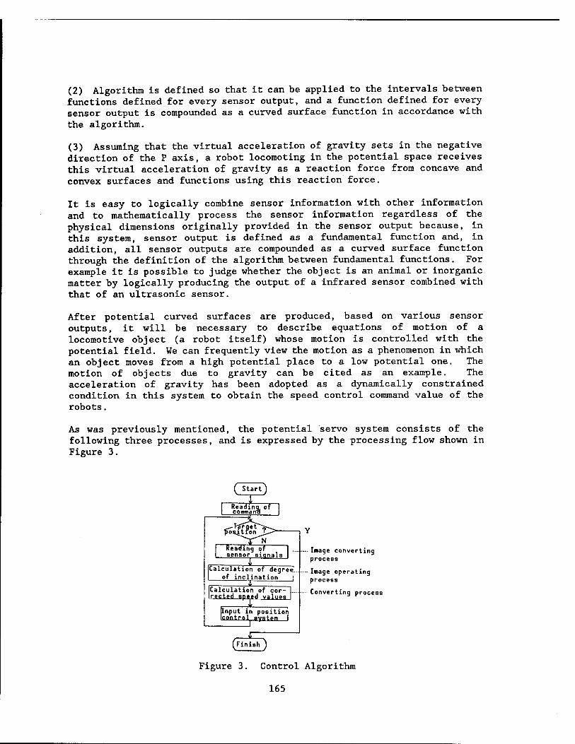
(2) Algorithm is defined so that it can be applied to the intervals between functions defined for every sensor output, and a function defined for every sensor output is compounded as a curved surface function in accordance with the algorithm.

(3) Assuming that the virtual acceleration of gravity sets in the negative direction of the P axis, a robot locomoting in the potential space receives this virtual acceleration of gravity as a reaction force from concave and convex surfaces and functions using this reaction force.

It is easy to logically combine sensor information with other information and to mathematically process the sensor information regardless of the physical dimensions originally provided in the sensor output because, in this system, sensor output is defined as a fundamental function and, in addition, all sensor outputs are compounded as a curved surface function through the definition of the algorithm between fundamental functions. For example it is possible to judge whether the object is an animal or inorganic matter by logically producing the output of a infrared sensor combined with that of an ultrasonic sensor.

After potential curved surfaces are produced, based on various sensor outputs, it will be necessary to describe equations of motion of a locomotive object (a robot itself) whose motion is controlled with the potential field. We can frequently view the motion as a phenomenon in which an object moves from a high potential place to a low potential one. The motion of objects due to gravity can be cited as an example. The acceleration of gravity has been adopted as a dynamically constrained condition in this system to obtain the speed control command value of the robots.

As was previously mentioned, the potential servo system consists of the following three processes, and is expressed by the processing flow shown in Figure 3.

sensor signals -it-

Calculation of degree of inclination I

Calculation of cor- rected speed valnn

Input in position control system I

■ Image converting process

- Image operating process

Converting process

(Finish )

Figure 3. Control Algorithm

165

(1) Image converting process: modifies fundamental functions, depending on sensor signals.

(2) Image operating process: obtains a curved surface function * by mutually functioning converted images.

(3) Operating process: calculates the inclination of potential fields and obtains speed command values by using the virtual acceleration of gravity.

3. Potential Servo Executing Process

3.1 Image converting process

This process determines the producing position and shape of the fundamental function P, defined in the potential space, on the basis of signals output by sensors.

For example, the information on the position of an obstacle, obtained through an ultrasonic sensor, merely shows a one-dimensional distance. Then, in the same way as conventional methods, it is converted into information on multidimensionally relative positions as viewed from the robot's characteristic coordinate systems. This method is the same as conventional ones up to this point.

First, the fundamental function P is defined for information on the relative position, obtained by using the above method. P becomes a nucleus for mapping sensor output in the potential space. The multidimensional normal distribution function shown in Figure 4 was used in the system. It is easy to mathematically analyze the normal distribution function based on an exponential function since the normal distribution function is continuous and can be differentiated for variables of state. Some methods of mapping sensor output on the potential space can be studied with this normal distribution function, and the following method was adopted for applicable examples of obstacle evading control using an ultrasonic distance sensor.

vsmmmm

Figure 4. Shape of Fundamental Function

Now, R is defined as shown in the following equation:

R2

where, X: Position of robot on characteristic coordinate system XA: Position of obstacle

166

The fundamental function P expressed by equation (1) is defined within the potential space as the function shown in Figure 4, which is the maximum for an obstacle's position.

P(R) - K*exp(-R2/2 a2) (1)

where K: proportional constant a: standard deviation

In addition, a potential curved-surface can be formed by successively defining such functions for every sensor output and by compounding these functions in the image operating process explained in the following paragraph.

On the other hand, if robots locomote in absolute spaces, potential spaces produced in this system will move in the same way since the potential spaces are based on the robots' characteristic coordinate systems. Also, potential values of arbitrary positions of robots on characteristic coordinate systems can be found promptly since potentially curved surfaces are defined only n sensor detecting domains.

Accordingly, this system can dynamically produce potentially curved surfaces on potential spaces in accordance with the robot's motion, and can control these robots while observing.

Robots can generate their loci autonomously and can move in environments while dynamically recognizing these environments.

3.2 Image Operating Process

This process compounds fundamental functions defined for every sensor output in the previously-mentioned image conversion process, summarizes them as a curved surface function *, equation (2), and defines potentially curved surfaces.

As mentioned previously, the mutually arithmetic sum, difference, product, and quotient among the functions can be expressed with equations (3) to (6), with all of their nuclei retained as exponential functions, and the differentiability and continuity are maintained since the nuclei of the fundamental functions are exponential functions (Figures 5 to 8).

Therefore, when fundamental functions are defined for every sensor output and are totaled, the environment surrounding a robot will be expressed as a stereoscopically potential field, as shown in Figure 1. In addition, even when the robot locomotes within this field, the field will change dynamically, and the robot can be controlled using real-time, since the field is renewed with every sensor output.

167

Figure 5. Example of Image Opera- tion (Sum)

Figure 6. Example of Image Opera- tion (Difference)

Figure 7. Example of Image Opera- tion (Product)

Figure 8. Example of Image Opera- tion (Quotient)

Operations are carried out only by using sums and differences, since only the ultrasonic sensor has been used as an environmental sensor up to now. However, considering operations among such sensors as infrared and pressure sensors, the product and quotient are promising as future operators.

* - SKi * exp(-Ri2/2ai

2)

pi + p2 - Kx * exp(-R12/2a1

z) + K2 * exp(-R22/2<72

2)

Pi " P2 = Ki * exp(-R12/2a1

2) - K2 * exp(-R22/2a2

2)

Px * P2 - Kx * K2 * exp(-R12/2a1

2 - R22/2a2

2)

V*2 - KiA2 * exp(-R12/2a1

2 + R22/2a2

2)

3.3 Conversion Process

(2)

(3)

(4)

(5)

(6)

This process obtains speed command values for robot locomotion by using the inclination of the potential surfaces produces.

Now, as a result of conducting the operations mentioned in the previous section, assuming that the potential surface is compounded in a shape like that shown in Figure 1, as shown in Figure 9, the inclination of an arbitrary point (point A shown in Figure 1 is regarded as an example of the arbitrary point) of the robots' characteristic coordinate systems is found per axis of the characteristic coordinate systems. Let's take one of the axes, axis X, as an example. As shown in Figure 9, the acceleration assigned to a robot at point A in the direction of this axis is decomposed and found in each axial direction on the assumption that the virtual acceleration of gravity is applied at point A in the negative direction (axis P).

168

p II

ü)

-G- Sin«

-*■ X

(b)

Figure 9. Calculation of Potential Grade

That is, the robot receives virtual force in the opposite direction according to the inclination of the surface. Accordingly, the robot can evade high potential sections, such as obstacles, and inductive force can be exerted so that the robot can be induced to low potential sections as a goal. Then, speed command values are made per axis by differentiating the obtained induction acceleration of the first order and by converting it into speed. When the robot can be controlled according to the speed command values, it will be possible for it to evade obstacles autonomously.

4. Applications to Practical Systems

4.1 Application to Obstacle Evasion Problems

.The application of this system to practical systems is being considered based on the methods explained previously.

The application of the system to autonomous obstacle evasion robots is being considered by using an ultrasonic sensor, a gyroscope, and an accelerometer. Such robots locomote in two-dimensional planes as moving spaces. (Figure 12 shows a system configuration of a locomotion robot.)

First, obstacles are detected by an ultrasonic sensor, which is an environmental sensor, and the position and posture of the robot itself are detected by a gyroscope and an accelerometer, which are state sensors. As shown in Figure 10, the ultrasonic sensor, gyroscope, and accelerometer are installed in the robot.

169

Ultrasonic senso<

OB)

Figure 10. Potential Space and Robot

First, obstacles are detected by an ultrasonic sensor, which is an environmental sensor, and the position and posture of the robot itself are detected by a gyroscope and an accelerometer, which are state sensors. As shown in Figure 10, the ultrasonic sensor, gyroscope, and accelerometer are installed in the robot.

Figure 11. Produced Potential Function

When the robot is positioned in an environment similar to that shown in Figure 10, the output of the ultrasonic sensor will be converted into the robot's characteristic coordinates at the coordinate conversion section shown in Figure 12, and the relative position seen from the robot is recognized, as shown in the figure. A target position is given to the robot

170

in advance, a relative position is found by using the target position while the current position is measured with a gyroscope and an accelerometer, and a concave section is formed on the relative position.

Unit vector

4- Ultrasonic

sensor

h-U Q—— transformation I "fa

Coordinate

(Transforma- tion to char acteristic coordinate)

ttm«qe protÜÜL Iduction ~

Rn

Jmaqe prof- Pt Tduciion I

J I {[mage pr tjuction

'co •H 0)

Pfl_

Target position XV,Yr "

Present .. .. acceleration *' ' *

Present speed of rotation

Target angle of rotation

iiii rpTtSJ

at a. a. x o 9t

Image conver- sion process

Virtual suctic -X 1 force K

OS

Image operat-

ing process

Mechanism for calcu- lating degree of lncllrf^tlft^ j r

Virtual gravity calculating machine

IVirtual torque Conversion section

Figure 12. Block Diagram of Potential Servo Control System

When convex sections formed in the position of recognized obstacles are piled on the concave section (image operating process), a potentially curved surface, similar to that shown in Figure 11, will be completed.

Then, the induction acceleration at the sensor installation position is found during the operation process by taking into consideration the fact that characteristic coordinates of the robot accord with coordinate systems of the potential space, except for axis P.

A position control system works in the robot. It is equipped with a gyroscope and an accelerometer independent of the above-mentioned gyroscope and accelerometer. Speed command values output by this system are corrected with the correction values output by a potential servo, and are output to the lower control system.

From the results mentioned previously, it can be said that the robot will autonomously trace evading loci against obstacles, and will be induced to approach the goal. We have confirmed the validity of this system by applying the system to an actual locomotion robot.

171

where

* - Zpq * expC-Rij2^2) (7)

Ri/ - (X, - Xj)2 + (Yi - Yj)2

(Xi( Yi); sensor installing position (Xj, Yj); position of obstacle

AVAX - SSKi/tJi2 * (Xi - Xj)

* expC-Rij2^^2) (8)

A*/AY - ESKi/CTi2 * (Yi - Yj)

* exp(-Rij2/2ai2) (9)

a - tan"1 (Atf/AX) (10)

ß - tan"1 (A*/AY) (11)

Fxi - -M * G/2 * sin(2a) (12)

Fyi = -M * G/2 * sin(2£) (13)

5. Conclusion

This system produces virtually potential curved surfaces on the basis of signals emitted from sensors, and induces the robot toward the goal by using the acceleration obtained from the inclination of the surfaces. It has been confirmed that the system is effective as an autonomous locomotion robot controlling method due to sensor feedback. However, many points remain for further study, e.g., the shape of fundamental functions, curved surface compounding methods, etc. Accordingly, in order to put the system to practical use, it is necessary to conduct further research on the system.

References

1. N. Hogan, "Mechanical Impedance Control in Assistive Devices and Manipulators," Proc. the Joint Automatic Control Conference August 1980, Vol 1. 5

2. Ibid., "Programmable Impedance Control of Industrial Manipulators," CAD/CAM Conf. in Mech. Eng., MIT, 1982.

3. Ibid., "Impedance Control of Industrial Robots," ROBOTICS AND COMPUTER-INTEGRATED MANUFACTURING, Vol 1, No 1, 1984, pp 97-113.

172

Tele-Vehicle I--Autonomous Remote Controlled Vehicle

43064062 Tokyo 4TH INTELLIGENT ROBOTS SYMPOSIUM PAPERS in Japanese 13/14 Jun 88 No 209 pp 115-120

[Article by Hideaki Ohyama and Akira Täte, Mechanical Engineering Laboratory]

[Text] 1. Introduction

The authors, et al. , have manufactured a remote controlled experimental vehicle, "Tele-Vehicle [TV]-1," have conducted research on remote control technologies, and have shown that complex work can be conducted by employing remote controlled robots, instead of humans, in their research laboratory. However, the work to be conducted by robots does not only involve complex work requiring human direction at all times. For example, the realization of autonomous control robots will relieve the human operation load in work which is relatively easy for robots to autonomously carry out, such as locomotion in familiar and unmanned environments.

This report describes an interactive environmental model-making system as an environmental model constituting method, which is one of the elemental technologies for enabling locomotion robots to autonomously carry out the work, and confirms the validity of this system. First, the TV-1 will be explained briefly and the environmental model-making system will be described.

2. Remote Control Experimental Vehicle (TV-1)

The TV-1 will be explained briefly.1 The TV-1 is a locomotion vehicle similar to that shown in Figure 1 [not reproduced]. Basically, the TV-1 is remote controlled by humans. The portion of the work previously done by humans is carried out by an autonomous vehicle, TV-1, but the TV-1 is not sufficiently autonomous to replace humans. Therefore, importance is attached to interfacing between the TV-1 and humans.

An autonomously locomotion system for the TV-1 is currently being manufactured. This system is comprised of an environmental model, interprets commands from humans on the basis of this model, makes a track plan, and transmits these commands to the TV-1 itself. The system is expected to have a configuration as shown in Figure 2.

173

■ CoHMand Interpreter

'Control 'Navigation

■a_

&—&

Host mputtr

Hunan interface

Environmental model control Track plan

Simulation

CoMiand generation Communication

Figure 2. TV-1 System

3. Model-Based Measurement System

Research involving the construction and use of environmental models is currently being conducted as an important subject for the field of robotics.2'3 Although the necessity for the use of environmental models has been advocated, the number of robotic systems using environmental models is not yet large. It is not easy to make general environmental models, which is one of the reasons that such models are not being universally employed. However, even if it is difficult to model general environments, it is easy to model specific environments, such as research laboratories, factories, and space. High-level functions can be expected in these places by making environmental models and adopting methods for taking action on the basis of these models.

Data on most basic environmental models show the three-dimensional shapes of buildings and objects, as well as their positions and attitudes. The view exists that conventional computer aided design [CAD] systems should be used to make environmental models, but conventional CAD systems are unsatisfactory since, although environmental models of buildings can be made by reading data in CAD systems, other factors in addition to building models which can be restored with design drawings are required for locomotion robots, even in relatively prepared environments, such as factories and research laboratories. Objects such as desks, chairs, and lockers exist in rooms, and objects are also placed in corridors. It is necessary to measure and register the position, attitude, and shape of these objects. Ideally, the robots would automatically carry out the measuring and registration, but it is currently very difficult for them to do so. Also, it is preferable that the human-robot system have an environmental model that can be understood by both the humans and robots.

Therefore, it will be necessary to develop a system which verbalizes environmental models by combining a conventional CAD system and a measurement system.*

Assuming that a parameter which should be estimated is x, the observed value is y, and the observation model is f(x), the measurement can generally be regarded as a process for estimating x, since the equation, y = f(x), holds. Now the following case will be considered. The shape, position, attitude, etc., of objects are to be estimated from images. Even when the same kind of observation quantity, called the "Vertex Position," exists, f(x) will change depending on the element, x and the kind of object. When identical objects are involved, the shape of f(x) will change according to which

174

object vertex is observed. However, after the shape, position, and attitude of the objects are defined with variables, if the observation model f(x) can be deduced from the definition of the object shape and that of the observation quantity, a general-purpose measurement system using images can be constructed. A system combining the measurement system and the CAD system has been called, "Model Based Measurement System." The environmental model-making system is an example of such model measurement systems.

Figure 3 shows the configuration of an environmental model-making system. This system is a subsystem of environmental model control systems which control environmental models of locomotion robots.

Observa- tion system

Inge input

Observa- tion, solving systen

Observation ■odel processing ayste»

Shane ■odel

Observa- tion nod* 1

Hunan interface

Inge . . indication

User input processing

Model editor

Figure 3. Configuration of Environmental Model-Making System

The environmental model-making system consists of a) a model editor which defines the shape model and observation model of the observed values, b) an observation system which inputs images into a computer, c) an observation equation synthetic system which deduces an observation equation from the observed values and the definition of shape and observation models, d) an observation equation solving system, and e) the human interface.

The environmental model-making system manufactured by the authors possesses the following features:

(1) The system defines the shape by using model description languages [MDLs].

(2) Variables can be used to describe models, and can be estimated by measurements. Therefore, shape variable objects, such as humans and chairs, can be defined.

(3) Even if the kinds of observation quantities change, the system can correspond to the change since the observation models of observation equations can be defined.

(4) If the system can observe, it will be able to estimate variables regardless of the observation quantities and kinds of variables which should be estimated.

(5) The known information and observation quantities can be combined by using the nonlinear least squares method.

175

(6) Environmental models are verbalized through a mouth while watching the shape models and input images. Observation equations are obtained by coordinating these shape models and input images.

(7) The three-dimensional position and attitude of objects with known shapes can be estimated from an image. Known information can be used in estimating the shape of objects. The known information can also be used to estimate the position and attitude of locomotion robots.

I I»aqt input

Renewal of envi

ronaiental aodel

End |

Figure 4. Estimation Procedure

Figure 4 shows the estimation procedure. It is necessary to make model functions of the observed values and to make models by using MDLs upon measurement.

An observation equation is obtained by reading shape models and observation models and by coordinating these models and input images. A variable which should be estimated is obtained by solving this observation equation. The estimated error is determined from the observation function and information on the errors of observed values. If the images and models overlap, the estimate will be successful, but if they do not, it will be a failure. In the case of failure, the estimate must be carried out again.

4. MDL

The MDL has been prepared to measure model-based images. The following functions are necessary for shape MDLs, which define the shapes of objects.

(1) Parametric function which can determine the shapes of objects, depending on variables.

(2) Function which exploits properties obtained from previously-defined models.

(3) Function which can define the shape of objects by using a set operation.

(4) Shape-defining function due to sweeping.

176

<*d«H»tlnltl»»>::=«w<tt-M»«> <iriuMit-blick> KJaclaratlon-tlack» «e«nilralU-»Uck» <iaaii-i"tietlatI»rrlU»»

<>r|dMnl-kl«k>: :*()! «•rtu«tnt-lUt>> <aflMtnt-IUt>::=<varlakla>

!<virUk|i><il|UMDt-lllt> !<»ri»«Bt-IIil> Ika» (<tai><varlaHt»

:<»rimnt-ll«l> »•HU»» I «variabla> <lala«ll-»alia»

cd«e\«f»l!on-bltck>:;= (itclait <4acl»r»llan-llat>) <«aelaratlan-llat>::=<Jaclaratlan>

:<dielaritl>n>«tcliratUn-llit> <daeliratl»n>::=«varlaHt> <ftf«>>

<«nttfalnti-»I«ck>::*<e«n«l»alntt <c«mtf»l»U-ll«I» <e»»itrilhU-IUt>::=<c«B«»ral»t»>

!<cen>llalnti><e»nilraliitt-ll(l> <eonitralnt>::=«eoiiitraliit-tya«> <ai|gm-ll»t-e» <«Mtfal«t-t»t>::= «!>!<(>«!<■

i nor«I ! iiiltar»

<»ri«»»nt-lltl-c>::* <f»r»> ! <lot»> <ar«iMnt-ll«t-c>

<»haaaHa»cfI»ll»n-IJit>:: = <ahaaa-daaerl»tl»a> !<ibaaa-d»icrlatl»n> <ihj»a-<latc r la t Un-I l> t>

<>hapi-4»crlprl«n>::<<tur(aca-a«ltl> !<«imr»llnJ-erllnJtr> !<tunetlo» !<«*<fal> :<centia|-tantanca>

<»grfact-Mdil>::s((v»rl»x«i <iartta-llat» Ulna» <llna-llst» (alaaai <»lana-llit»>

<H4II>: : = (<■♦<• 1 -n»nc> <ariunnt-llst>)

<funeU<m>::*(<funelar> <ari«Mnt-llit-(>) <functlor>::= »cala ! aova ! rotata ! aari»

i or <»riuiinl-liit-l>::»<vaet»l>

!<vtclor><ariumnt-IUt-f> !<*haaa-4aier l»t lan-l U l> !<tliaa*-4ticrlarl»n-lltl> <ariu»«nt-ll«t-f>

<toatn>l-niit«nce>: : = (J»r (<varlakl«> <litltlal-valu«>

<tanlnal-valut>> <ikaBa-iaicrlarleii-lltt»

<M»«ur»atnt-wdtI-<lef lalilen>:: = KMasuraannt-Mdal-naia> <ariuiaant-lltt>

<iaaatura»fRt-a»a'al»

Figure 5. Model Language Description (Essentials)

177

(5) Deformation by Euler's operation.

This system possesses (1), (2), and a portion of (4) above. The function mentioned in item (1) has been expanded over that of conventional CAD systems. The system does not process any data on numerical values, but processes functions which output shape models as data. Figure 5 shows specifications of the system. The function described with MDL does not output any data on vertex numerical values, but outputs variables which should be estimated as arguments.

(rectangular (x y) (vertexes(l (x y 0)) (2 ((-x) y 0))

(3 ((-x) <-y) 0)) (4 (x(-y) 0))) (lines(1 (1 2)) (2 (2 3) (3 (3 4)) (4 (4 1))) (planes(l (12 3 4)) (2 (1 4 3 2))))

Figure 6. Surface Model of Rectangle

Figure 6 shows the most primitive sentences. These sentences express a rectangle as a surface model. Models are defined by combining such primitive sentences. Figure 7 shows the description of a desk.

(desk (x y r h &optional(dx 0.03) (dy 0.03)) (declare(x2 (- (/ x 2) dx)) (y2 (- (/ y 2) dy))

(array leg (legl leg2 leg3 leg4)) (array legpos ((x2 y2 0) ((-x2) y2 0)

((-x2) (-y2) 0) (x2 <-y2) 0)))) (board (move (0 0 h) (rectangularxy))) (for (i 1 4)

((leg i) (move(legpos i) (cylinderr h)))))

Figure 7. Example of Description of Desk

5. Description of Observation Model

Observation quantities in images are multiform, for example, the position of the vertex, linear equation, axis of a cylinder, radius of an ellipse, etc. The measurement system must be able to define model functions of these observation quantities.

If the position of the vertex of objects on an image plane is expressed with a function, such as the Lisp function, on the assumption that the position and attitude of these objects and those of a camera are described with an absolute coordinate system, the following items can be obtained: 1) perspective transformation--lens characteristics; 2) inverse rotation-- position of camera; 3) inverse translation--attitude of camera; 4) translation--object positions; 5) rotation--attitude of objects and coordinate of vertex of objects. The inverse rotation and inverse translation refer to the inverse transformation of rotation and translation, respectively. When they are defined using MDLs, observation models are defined by combining transformation functions, such as translation,

178

rotation, perspective transformation, etc., with functions which derive vertex coordinates and coordinates of both ends of line segments from models. When all arguments are numerical values, they will be evaluated as normal Lisp functions in the observation models. When arguments include variables, they will not be evaluated. It is not until the value of these variables has been determined that the arguments will be evaluated.

6. Coordination

The position of objects on input images can be obtained by pointing the dots of these input images. When shape models are displayed by substituting appropriate values for variables, when the dot corresponding to the vertex of these shape models is pointed in the image plane and when observation models of the vertex of the shape models are combined with the vertex position of the images input observation equations will be obtained. The linear case is the same as was mentioned above.

Even if the straight lines and model vertex specifications deviate slightly, the deviation will not pose any problems since these straight lines and vertices have been selected from input values, minimizing the distance between the straight lines and the vertices. However, the specifying of such straight lines and vertices on input images must be carried out with high accuracy since this specification will directly bring about observed values. Figure 8 [not reproduced] shows an image plane at the time of coordination.

7. Observation Equation Solving System

Observation equations are solved in accordance with the following procedures. A flowchart is shown in Figure 9.

(1) Receive lists of restricted conditions, data on observation error, observation equations, and variables which should be specified.

(2) Add these restricted conditions to the list of the observation equations in accordance with the kind of restricted conditions.

(3) When variables not included in observation models exist, check for no observability.

(4) When observation equations and variables can obviously be divided into classes, carry out the division.

(5) Check to see if observation equations can be solved with a solution defined by the users. When they can be solved with the solution, start its routine.

(6) Start using the nonlinear least squares method.

(7) Estimate the accuracy from the Jacobian matrix for observation models and data on the errors of observed values.

179

Input of observi tion equipment

Processing of restricted CBndmong

.necking of )bssrv»bility

Problem division

Solution defined by u»»r» I

Figure 9. Solution of Observation Equation

Generally, it is difficult to analytically solve nonlinear simultaneous equations. Even if they can be solved analytically, it is very difficult to obtain the optimum estimate by combining information on errors of observed values with known and restricted conditions. Accordingly, this system adopts the nonlinear least squares method as a main solution.

In the case of nonlinear problems.it is difficult to analytically investigate the observability. However, when the number of variables is smaller than that of observation equations, or when the variables are not mentioned in the list of observation equations, there will be no observability. Therefore, warnings will be given to users, and the input of new observation equations will be promoted. The final determination of observability is carried out by using the nonlinear least squares method and the Jacobian matrix.

In order to solve problems by using the least squares method, it is necessary to use information on the observation model, the error distribution of the observed values, the observed values, the initial values of variables which should be specified, and these variables themselves. In the case of nonlinear problems, there is no assurance that these problems can be converged into a true solution. That is, they may be converged into a locally minimal solution. Therefore, it is necessary to provide a number of initial values.

The Marquardt method is used as an algorithm for the nonlinear least squares method.5. The Marquardt method requires Jacobian matrices for observation equations, but, except for special cases, observation equations can be found

180

using the difference approximation. The Jacobian calculation speed based on the difference approximation is low, but the accuracy is the same as that of analytical calculating methods.6

8. Handling of Restricted Conditions

In the case of monocular vision, it is difficult to estimate variables which express dimensions without any known information. Measurements can be carried out while moving a camera, but this system is used to measure fixed points. In order to measure variables expressing dimensions, it is necessary to use known information. For example, information on desks and chairs can be used, because their dimensions have already been determined. However, it is necessary to be careful when using such information. Measurement accuracy depends on the precision of known information.

The following items can be cited as expressions of known information.

(1) The probability distribution of values of expressions. (2) Equality restricting conditions. (3) Inequality restricting conditions. (4) The domain of definition of variables in the special case termed "Inequality Restricting Conditions."

It is difficult to handle the probability distribution of general expressions. Practically speaking, it is believed that the handling of uniform and normal distribution will be satisfactory. When the probability distribution of values of expressions is normal, it is easy to handle the normal distribution by using the least squares method. These expressions should be added as observation equations to observation vectors. When the probability distribution of values of expressions is uniform, or when it has inequality restricting conditions, the probability distribution must be handled with a penalty method. Domains of definitions of expressions and inequality restricting conditions are added as penalty function arguments to observation vectors. In the case of inequality restricting conditions, a variable is converted into another variable, if possible, with these conditions, while, if impossible it is added as a penalty function argument to the observation vectors.

9. Solution Defined by Users

This system can find the value of variables numerically from the value of observation quantities and the relationship between the observation quantities and variables, which should be estimated. However, if the value of these variables can be found analytically, in many cases the value can be solved stably at a high speed, and no uncertainty is caused when the value is solved numerically. As mentioned above, the value of the variables is found analytically from a relationship between the observation quantities and variables. This is a kind of mathematical expression processing method. Then, ideally, it is necessary to incorporate mathematical expression processing technologies into CAD systems for measurements. Currently, the above system does not possess any mathematical expression processing function, but when problems requiring solutions can be solved with a

181

solution defined by the users, the solution can be initiated. For example, of four points of an object having a known shape, which exists on a plane, can be coordinated, the attitude and position of the object can be estimated analytically. If those of one which does not exist on a plane can be coordinated, the approximate solution of the attitude and position of the object can be found analytically. If the nonlinear solution is used for the above estimation and approximation solution as initial values it will be possible to carry out estimates with high accuracy and high speed.

With regard to lists of variables, observation equations, initial values, etc., for initiating the nonlinear least squares methods, if a pattern obtained by matching patterns can be solved with a user's solution routine, the user's solution routine will be initiated. Finally, results obtained by starting the routine will be transferred to the nonlinear solution.

10. Specified Accuracy

It is difficult to briefly mention the measurement accuracy, since it varies depending on the object of measurement, the method of selecting the vertex and straight line, and specific variables involved. However, in individual cases, the measurement accuracy can be estimated from observation equations and observation noise. Assuming that the parameter which should be specified is x, and the observed value is y, the observation equation is

y - h(x)

H is the Jacobian matrix,the covariance matrix of observation error is ZL, and the error covariance matrix of the parameters is

2, - (H1^/1 H)'1

The observation error is not always expressed in normal distribution since, in this system, measurements are carried out by humans. Also, the distribution of errors changes depending on the situation, and it is necessary to be attentive to this change.

11. Image Measurement by Monocular Vision

The shape, attitude, and position of models are estimated from an image in this system. It is difficult to find both the shape and absolute distance, since measurements by monocular images bring only a small amount of information. However, in the following relatively useful case, it is possible to carry out measurements.

When objects with known shapes are used, and when the number of points coordinated between the interior of the model and the image is more than three, the three-dimensional attitude and position of these objects can be measured.7 Inversely, when the shape of the objects is known and when the position of these objects is known, the three-dimensional attitude and position of the objects can be estimated. Measuring the initial state of locomotion robots is relatively complex, but the state of these locomotion robots can be readily estimated by measuring using images.

182

Even if the objects are rectangles and their dimensions are unknown, the attitude and aspect ratio can be estimated by observing four points. However, the absolute distance and dimensions cannot be solved. Also, if either the longitudinal dimension or lateral dimension can be solved, the remaining dimension and the position can be measured.

It is permissible to assume that the robot is on a flat plane in environments in which the motion of robots can be specified on two- dimensional flat planes, such as inside factories. In this case, a total of variables should be estimated since the position has two degrees of freedom and the attitude has one degree of freedom. The position and the attitude can be estimated by observing two points.

12. Experimental Results

Here, estimation results will be described for some examples. The estimates have been carried out using this system, and the input images and models overlap.

(1) Example 1

Figure 10 [not reproduced] shows the results of estimating the position and attitude of a desk. Six vertices were coordinated. The estimated error of the attitude was an RSS error, and was 2.4 degrees. The positional error has not been measured.

(2) Example 2

Figure 11 [not reproduced] shows the results of estimating the three- dimensional position and attitude of a locomotive robot. The vertical line of the wall and the horizontal line of the illumination were coordinated. The attitudinal error was an RSS error, and was 3.2 degrees. The positional error was 12.5 cm.

(3) Example 3

Figure 12 [not reproduced] shows the results obtained by using a human model, by estimating the articulation angle as a variable, and by overlapping the human model and an image. The total number of variables was estimated to be 25 by adding the 19 variables showing the articulation angle to the 6 variables indicating the position and attitude of the body.

13. Conclusion

The nonlinear least squares method requires much time since the expression of the system uses the Lisp function. We are currently carrying out a study in which the Lisp function is turned into a c function, since the c function can be called from the Lisp function. We are also conducting a project in which observation models can be output as c functions by processing these observation models.

183

The system is currently being used to carry out measurements from an image, but image measurements by monocular vision involve many restrictions. It is particularly difficult to measure objects with unknown shapes. However, it is necessary for the system to be able to measure objects with unknown shapes. If the system is equipped with a distant sensor it will be easy to estimate shapes, and it is believed that the system employing a distant sensor will take a step forward toward practical use.

Restricted conditions are currently handled with a penalty method, but the use of the penalty method may cause numerically unstable states to occur. This method will be modified in the future.

This system can also be used as a system to recognize images.

References

1. Täte, et al., "The Seventh Report, Research on Tele-Existence--Remote Controlled Locomotive Robot Having Presence," The 25th Measurement Automatic Control Society Scientific Lecture Meeting Pre-Journal.

2. Shirai, "Model Based Vision," JAPAN ROBOT JOURNAL, Vol 2 No 6, 1984, pp 89-94.

3. Shirai and Inoue, "View of Intelligent Robot--Model Based Robotics," Ibid., Vol 5 No 6, 1987, pp 462-469.

4. Hasegawa, "Modeling and Monitoring of Robot," MEASUREMENT AUTOMATIC CONTROL SOCIETY PAPERS, 17-5, pp 489-595.

5. Nakagawa and Koyanagi, "Experimental Data Analysis by the Least Squares Method," Publishers' Association of the University of Tokyo, 1982.

6. K.I. Hiebert, "An Evaluation of Mathematical Software That Solves Nonlinear Least Squares Problems," ACM TRANSACTIONS ON MATHEMATICAL SOFTWARE, Vol 7 No 1, 1981, pp 1-16.

7. Koyama, "Relative Navigation System Using a Number of Camera Images," Perceptual Organization and Visual Recognition," 1985, Kulwer Academic Publishers

184

Capture Operations Involving Orbiting Space Robot Manipulators

43064062 Tokyo 4TH INTELLIGENT ROBOTS SYMPOSIUM PAPERS in Japanese 13/14 Jun 88 No 111 pp 121-126

[Article by Youji Umetani and Kazuya Yoshida, Tokyo Institute of Technology]

[Text] 1. Introduction

The age of full-scale space development has arrived, and space robot technologies are in the limelight. It has been pointed out that technologies for robots and automation will have to constitute the main keys to relieve workers (astronauts) from dangerous labor called for in the extreme environment of "Space," and to promote the effective use of space while raising the working efficiency.1,2 Specifically, the unmanned satellite system with an autonomous manipulator can be regarded as an intelligent locomotion robot which can freely fly in space, and the importance of research and development of such space-related intelligent locomotion robots is very high.

The conceptual study of robot systems for use in space environments was started in the 1970s in the United States,3 and such a robot system was first put to practical use as a manipulator system in the Space Shuttle.* Since then, other countries have conducted research on space robot manipulators, with Japan also promoting the basic research and development of space station manipulators5 and orbital servicing vehicles [OSVs]. Specifically, the latter functions as an intelligent locomotion robot for use in space, as mentioned above, and is very interesting.

Incidentally, it is necessary to be on the alert for new problems that could be caused by the difference between environmental conditions on the ground and those in space when conducting the research and development of space robots. In general, orbital environments have 1) a substantial vacuum, 2) severe thermal conditions, and 3) minute gravity. Many technical subjects must be solved, since problems peculiar to each condition will occur. Of the three items above, the following two problems caused by item 3) are important from the standpoint of robot control.

(1) It will become possible to manufacture huge structures since they will not need to support their dead loads in minute gravity environments. Also, these structures are designed so that they will be significantly lightened

185

when their rockets are launched due to the weight limit. As a result, large robot arms and large structures, such as space stations, will essentially become flexible structures with low rigidity and will require damping control.

(2) An immovable foundation, which should become a standard, cannot be obtained since all objects are in a floating state while orbiting. That is, the rotation of the manipulator arms will cause a reaction that will move the foundations fixing these arms. For example, when a manipulator is mounted on a satellite, the attitude movement of the satellite itself will be disturbed by the movement of the manipulator.

Of the above two problems, research on the first is being vigorously conducted in various fields, while this paper tackles the second problem and describes detailed movement control of rigid body manipulator systems in orbit.

The accurate operation of manipulators is interrupted by the reaction to the spaceship bases caused by the movement of these manipulators. This matter is not as serious when astronauts carry out work on the relative coordinate systems fixed on spaceships, but when an object in orbit, such as that shown in Figure 1, is caught, it is necessary to operate a manipulator along the target orbit described on the inertial coordinate system fixed in space. In this case, it is necessary to be able to control manipulators due to the reaction caused by spaceships.

Research on the modeling of some space manipulators has been conducted in the past7"9 and, as shown in Figure 1, when capturing objects is considered, it is necessary to solve an inverse kinematic problem involving floating rigid body systems. The authors, have paid attention to this problem, have formulated the kinematics of space manipulators installed on floating satellites, and have proposed a new kinematic theory for space manipulators in which reaction dynamics is taken into consideration. The basic philosophy of the new theory has already been described in the references mentioned later in items 1) and 2). Now, the authors will describe the detailed process of deducing the new theory, show a simulated result of a model of a certain robot satellite, and study problems involved in catching and controlling orbiting objects and in controlling spaceship attitude.

2. Formulation of Problems

2.1 Description of Problems

This paper tackles the task of catching a floating target, as shown in Figure 1, as important for space robots. In order to execute the catching motion, it is necessary to give a target or bit as a tool to the catching motion and to find the articulation motion necessary to realize the catching motion, i.e., it is necessary to solve so-called reverse problems. It is very interesting to solve them analytically.

Incidentally, if the position and attitude of satellites can be controlled in orbiting satellite manipulator systems so that these satellites are fixed

186

Figure 1. Schematic Illustration of a Capture Operation in Orbit

completely in inertial space, manipulators mounted on the satellites can be handled similarly to those fixed on the ground. One method is to study the control of the position and attitude of such satellites, but the authors think that this is a dynamically special case. In this paper, the authors believe that a general case would involve interference being generated between both motions without any satellite control, the entire satellite- manipulator system being formulated by regarding it as an articulated rigid body link system floating in space, and a solution to general reverse problems being studied.

2.2 Assumptions

The following assumptions have been made to clarify points of discussion.

(1) A robot satellite is mounted with a rotating articulated manipulator having n degrees of freedom. Also, all systems consist of rigid bodies.

(2) The systems are floating in inertial space, and the dynamic conservation law holds without any external force reacting. Also, the position and attitude of the satellite itself are not controlled.

(3) All states of the systems are observable, and the capture orbit necessary to solve reverse problems is given to inertial space in advance.

2.3 Establishment of Model and Variables, and Coordinate System

The model and variables are established as shown in Figure 2. The main variables are as follows:

p:i : Barycentric position vector at each articulation trG : Barycentric position vector of the entire system IPn : Position vector at the top of manipulator £L, eiL, |b±: Vectors which show length of each articulation and

barycentric position

187

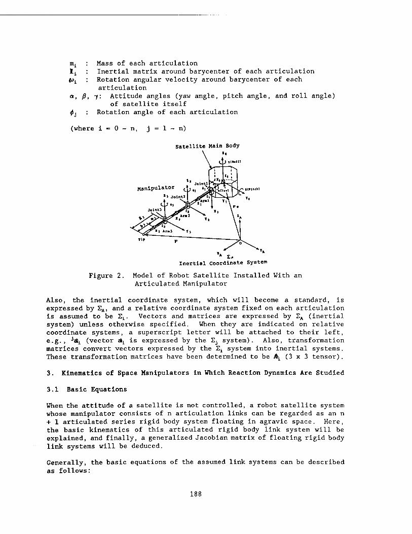
mi

ß,

*i ■

(where i

Mass of each articulation Inertial matrix around barycenter of each articulation Rotation angular velocity around barycenter of each articulation

7: Attitude angles (yaw angle, pitch angle, and roll angle) of satellite itself

Rotation angle of each articulation

0 - n, j = 1 - n)

Figure 2.

Satellite Main Body

«. J Yl»olll

Jotntl Manipulator ^ f> r

*» Joint]

Inertial Coordinate System

Model of Robot Satellite Installed With an Articulated Manipulator

Also, the inertial coordinate system, which will become a standard, is expressed by SA, and a relative coordinate system fixed on each articulation is assumed to be 2L. Vectors and matrices are expressed by EA (inertial system) unless otherwise specified. When they are indicated on relative coordinate systems, a superscript letter will be attached to their left, e.g., iäL (vector Ai is expressed by the Sj system). Also, transformation matrices convert vectors expressed by the 5^ system into inertial systems. These transformation matrices have been determined to be AL (3 x 3 tensor).

3. Kinematics of Space Manipulators in Which Reaction Dynamics Are Studied

3.1 Basic Equations

When the attitude of a satellite is not controlled, a robot satellite system whose manipulator consists of n articulation links can be regarded as an n + 1 articulated series rigid body system floating in agravic space. Here, the basic kinematics of this articulated rigid body link system will be explained, and finally, a generalized Jacobian matrix of floating rigid body link systems will be deduced.

Generally, the basic equations of the assumed link systems can be described as follows:

188

[Definition of barycentric position of the entire system]

Zmi r £ =ra Znu (1) Ml Ml

(2)

[Translational linear momentum conservation law]

n . Em* T i =const. Ml

[Angular momentum conservation law]

Z (I l tot +nw TL Xri) =const. '■*) w

[Geometric joint condition of articulations]

ri-r£.i=aj+bj-i (^)

[Characteristic equation of manipulator]

n (5) P = ro +bo + ZHi

M

Items (1) and (4) are simultaneous equations concerning barycentric position vector (Ti at each articulation. The following equation can thus be obtained:

TV

r i = ZK*j (Ai i a i + Ai-i^hi-i) +ra M (6)

where, coefficient KLi is a function of the mass ratio of each articulation. By differentiating equation (6) with respect to time, ti can eventually be solved as follows:

n ri=Evij*j+Va

M (7)

Also, VG is the initial velocity of the systems gravity, and is constant as long as external force does not act on the systems.

On the other hand, angular velocity fc^ around the gravity of each articulation can be expressed by a figure like that shown in Figure 2 on the basis of a simple geometric relationship:

n • tui =Z (Aj Juj) 0 j +oo

*• (8)

where, jUj is a unit vector which shows the axis of rotation of the jth articulation, and fc>G is the initial angular velocity of the entire system around the system gravity.

189

As mentioned previously, both iL and (^ can be expressed by a linear combination using angular velocity ^ of the articulations.

3.2 Characteristic Equation of Manipulator

Generally, the characteristic equation of conventional manipulators can be expressed as follows:

P-f<*> (9)

where P= (*>nT . 6TVT ) T

9n :

As is well known, the above relationship is linear, and its solution depends greatly on the state of the manipulators. The relationship obtained by differentiating equation (9) is as follows:

P = J(*>* (10)

However, in equation (10), the angular velocity # of the articulations and velocity IP in hand can be described by a simple algebraical relationship by using the Jacobian matrix, J (♦) =3f/9| . The angular velocity of the articulations of manipulators can be found against the velocity target value given in the working space based on equation (10). This method is known as a resolved motion rate control [RMRC]. It is also known that Jacobian matrices which appear in the method play an important role in analyses of the mechanism and operational properties of materials. Then, the kinematics of space manipulators is analyzed based on the RMRC philosophy.

Differentiating equation (5) with respect to time gives the following equation:

• • n P = ro +A (Ao °bo ) +ZA (.At iJU)

(ID

Jacobian matrices of conventional ground manipulators can be obtained immediately from the third term of the above equation, but a term concerning the attitude angular velocity and barycentric velocity of a satellite itself is added to the above equation. Also, the satellite itself is a manipulator installation foundation. These terms can be readily deduced as linear functions of i> from equations (7) and (8), and the entire right side of equation (11) can be expressed by a linear combination of • • • • • • • ♦ =a. ß, r. 0ii 0a . . . 0n.

190

P« "J (♦> **r.

■r* J» jT j4, - j*n

Atk A. i A. 1 Aik- A»k

where % P0 = (V« T , tUQ T ) T

(12)

K id, used in equation (6), is used to deduce equation (12). That is, a new Jacobian matrix J8 , defined in equation (12), is a function of the mass ratio of each link, and essentially satisfies the geometric condition, equation (1), concerning the barycentric position of the entire system. Also, equation (12) can be described as follows by dividing it into the satellite section and manipulator section:

• • • * P=/s *s + Jn 4M +PO

where t

Js (nx3 wtrix) , JM (nxn wtrlx) , **= (a, ß, r)T,

3.3 Conservation Law of Linear Momentum

(13)

Equation (13) is a basic expression important for describing the kinematics of floating rigid body link systems, and gives only n-degree independent equations against variables of ff>s (3 degrees), $M (n degrees): n + 3 degrees total. The motion of each articulation is restricted by a mutual reacting force in floating rigid body systems on which external force does not act, and j^s and f>M cannot be determined independently. In order to describe the relationship between them, it is necessary to consider the dynamics of the entire systems.

It is generally the case that the balance between force and torque is described to study dynamics, but this case becomes very complex. Incidentally, paying attention to the fact that the momentum of entire systems is conserved in those on which external force does not act, it will become possible to make arguments at dimensions of inertial term • velocity (angular velocity) = momentum (angular momentum), and it will become very easy to formulate the above momentum.

Arranging equations (2) and (3) by using the relationship between equations (7) and (8), the conservation of momentum can be summarized eventually, as shown in the following equation:

C/a /» IT /♦, /♦.] =1,0 ! i

*K

(14)

191

Inertial term 11^ which appears in the above equation is obtained by projecting the intensity of inertia against rotation <f>i in the working coordinate space. Similarly to equation (12), equation (14) can be obtained by combining the satellite section and manipulator section, and is shown as follows:

/t *t+/n ♦« =Lo (15)

where, to 13x1 vector) . initial angular momentum

/s (3x3 Mtrlx) , In (3xn utrlx)

3.4 Generalized Jacobian Matrix of Floating Rigid Body Link System

Two important basic expressions, (13) and (15), were obtained from the above-mentioned theories. They are simultaneous linear equations with three unknowns involving the n + 3 variables jj>s, jf>M. Incidentally, in order for the kinematics of manipulators to be achieved, it is necessary to explain the relationship between working space variable P and articulation space variable /H. Now, solving equation (15) with respect to ^s gives the following equation:

Substituting this equation for equation (13), the following equation can be obtained:

P = (.JH-JS /«^/M) *H+PO (17)

where, constant term, Po + «ft/t-1Lo is newly set as |P0.

Equation (17) describes the relationship between the articulation space and working space of floating multibody link systems, and implicitly includes the influence of the reacting motion on satellite sections. The intensity of the influence is shown with equation (17), with J» JS_1JM and K^ used when each term is deduced. For example, when the inertia of the satellite sections is very large, the following equation will be obtained:

That is, equation (17) will be changed to P = J*M , and will become the same equation as the kinematic equation for ground manipulators. This matter can probably be understood clearly by regarding the ground manipulator as a link system fixed on a large foundation, "Earth," which has an extremely large mass.

That is, it can be said that equation (17) is a general expression for the kinematics of floating rigid body link systems, including conventional manipulators fixed on the ground. Then, rearranging the term in equation (17) in parentheses, calling it the "Generalized Jacobian Matrix of Floating Rigid Body Link Systems," and presenting it with JH*, we obtain the following equation:

P=,r**M+Po (18)

192

When there is no redundancy between the working space and articulation space, J* will be changed to a square matrix of n x n, inverse matrices will be found in points other than singular points, and the inverse transformation of equation (18) will be given as shown in equation (19):

#M= CJ*:i-* (P-Po > (19)

Inverse kinematic problems can be found analytically, regardless of the existence or lack of a reacting motion of the satellite sections. This matter provides an important element to the motion control of space manipulators.

4. Study of Acquisition Control Problems

At this point, acquisition control problems will be studied by computer- simulating a model of a robot satellite assuming the above-mentioned formulated equations.

Basically, three degrees of freedom have been selected for the manipulator, while three degrees of freedom for the wrists have been omitted for the sake of simplicity. The values shown in Table 1 are supposed as the specifications of a realistic robot satellite. If the manipulator is operated along an orbit supposed arbitrarily from the certain initial posture shown in Figure 3(a), the speed in hand along the operation orbit at this time can be given as shown in Figure 3(b).

Table 1. Specification of the System

Satellite Manipulator link 0 link 1 link 2 link 3

nass (kg) 2,000.0 20.0 50.0 50.0 / (m) 3.5 0.25 2.5 2.5 Jx (kgm2) 1,400.0 0.10 0.25 0.25 J[y (kgm2) 1,400.0 0.10 10.4 10.4 iz (kgm2) 2,040.0 0.10 10.4 10.4

Initial Posture

X ,p Target Point

S Capture Trajectory 10.0 20.0 30.0

time ( sec ) (0.0

Figure 3(a) Figure 3(b). Motion Rate of the Tip

193

4.1 Case When Satellite Itself Is Not Controlled

First, the following case is studied. In this case, the satellite is engaged in reacting motion since it exerts no control over its position or attitude. Figure 4(a) and (b) show results of solving reverse problems by using equation (19). As is clearly shown in these drawings, the reacting motion of the satellite is unexpectedly large. The attitude is changed by about -23 degrees around the roll axis and about 14 degrees around the pitch axis during the assumed manipulator operation, with translational motion generated simultaneously during this operation. However, it can be appreciated that the top of the manipulator's hand catches the target orbit precisely, in spite of the reacting motion generated from this foundation.

The final position and attitude of the satellite itself due to reacting motion depend on the course followed by the top of the manipulator's hand. Also, when the satellite is in motion following the identical course, the identical results will be obtained regardless of the motion speed. That is, it is necessary to keep in mind that however slowly the manipulator may be operated, the change of the position and attitude due to the reacting motion is inevitable.

it-J.0(»«c)

10.0 »1.0 30.0 time ( sec )

«0.0

Figure 4(a). Course of Posture Change (Free-Flying Case)

Figure 4(b) Rotational Motion of Satellite Main Body

4.2 Attitude Control Problems

Next, the following case is studied. In this case, the attitude of the satellite itself is controlled during the operation of the manipulator. At first the formula mentioned in Chapter 3 was promoted on the assumption that the satellite itself was not controlled, but it is possible to simply apply the formula to an attitude control problem.

This problem can be treated as a case in which the angular momentum of the satellite side is controlled arbitrarily by mounting a reaction wheel on the main body of the satellite. Rearranging equation (15) on the assumption that (^ is the reaction momentum which should be added to the satellite to control its attitude, we have the following equation.

Is *s +/M *M+LC=0 ♦ s =0

(20)

194

Momentum IL^, which should be added to the satellite during manipulator operation, can be found by simultaneously realizing equations (20) and (13) and by substituting ls - 0 (attitude change of satellite - 0) for the simultaneous equation.

LC=-/M/M"1(P-P0) (21)

Also, the inverse kinematics of the manipulator at this time can be found using equation (22) by substituting /s - 0 for equation (13):

♦ ,=0 (22)

Figure 5 shows the results of solving the previously-mentioned acquisition control problem by using two equations, (21) and (22). Figure 5(a) shows the motion of the entire system at this time. The attitude of the satellite is fixed, but transitional motion occurs. Figure 5(b) shows the reacting angular momentum calculated with equation (21). Figure 5(c)shows the results obtained by differentiating the reacting angular momentum with respect to time and by finding it as a control torque. Performances required of the reaction wheels to be mounted on the satellite can be confirmed by studying such simulations.

4t-2.0(«ac)

Figure 5(a). Course of Postural Change (Attitude Control Case)

1.0 10.0 20.0 30.0 time ( sec )

(b)

u.o

Figure 5(b). Required Counter Momentum

195

i

u o

10.0 20.0 30.0 time ( sec )

(0.0

Figure 5(c). Required Counter Torque

5. Conclusion

In this paper, the solution to inversely kinematic problems was deduced analytically by modeling a satellite system, on which a manipulator was mounted, as a rigid body link system floating in inertial space.

The acquisition problem of floating targets was taken up as an example of a typical inverse problem involving space materials, and the usefulness of the methods proposed was shown through computer-simulations.

The reacting motion generated in the satellite is shown through simulations in which a realistic model is assumed. It has been confirmed that this reacting motion is of such magnitude that it cannot be ignored, and a very large capacity reaction wheel is required to control the reacting motion. The manipulator is controlled purposely while allowing the reacting motion mentioned in the paper. Therefore, it can be assumed that the manipulator controlling method is very effective for the case when the controlling capacity at the satellite side is limited.

Also, the magnitude of the influence of the reaction depends on the operating orbit of the manipulator, and one of the subjects of future research will be to study the operating orbit that will minimize this influence.

References

1. "Advancing Automation Robotics Technology for the Space Station and for the U.S. Economy," NASA-TM-87566, 1985.

2. "Report on Results of Automation Research Forum and Robotics in Space," Space Environmental Use Promotion Center, 1988.

3. Stanley Deutsch and Wald Heen, "Manipulator Systems Extend Man's Capabilities in Space," ASTRONAUTICS & AERONAUTICS, June 1972.

4. D. Gossain and P. Smith, "Structural Design and Test of the Shuttle RMS," Proc. of AGARD Conf, No 327, 1983, pp 2.1-2.10.

196

5. Yamamoto, Kuraoka, Iikura, et al. , "System Study of Japan Experimental Module Manipulator System," the Third Space Station Lecture Meeting, 1987, pp 49-50.

6. Iwata and Honma, "Requirement of Functions of OSV," the Third Space Station Lecture Meeting, 1987, pp 101-102.

7. K. Yamada, K. Tsuchiya, and S. Tadakawa, "Modeling and Control of a Space Manipulator," Proc. 13th ISTS, 1982, pp 993-998.

8. R. Lindberg, R. Longman, M. Zedd, "Satellite-Mounted Robot Manipulators--New Kinematics and Reaction Moment Compensation," ROBOTICS RESEARCH, Vol 6 No 3, 1987, pp 87-103.

9. Z. Vafa and S. Dubowsky, "On the Dynamics of Manipulators in Space Using the Virtual Manipulator Approach," Proc. IEEE Int. Conf. on Robotics & Automation, 1987, pp 579-585.

10. Umetani and Yoshida, "Acquisition of Floating Objects by Using a Satellite With a Manipulator--Part 2: Formation of Kinematics," the 25th Measurement Automatic Control Association Science Lecture Meeting Pre-Journal, 1986, pp 691-692.

11. Y. Umetani and K. Yoshida, "Continuous Path Control of Space Manipulator Mounted on OMV," ACTA ASTRONAUTICA, Vol 15 No 12, 1987, pp 981-986.

197

Development of Intelligent Robot for Nuclear Power Station

43064062 Tokyo 4TH INTELLIGENT ROBOTS SYMPOSIUM PAPERS in Japanese 13/14 Jun 88 No 112 pp 127-132

[Article by Ryouichi Nakayama, Katsuhiko Satoh, Satoshi Okada, Kazuhiro Tsumura, Hisashi Hozeki, Katsumi Kubo, and Akira Abe, Toshiba Corporation]

[Text] 1. Introduction

In recent years, the importance of nuclear power plants has increased as fundamental electric power generating facilities for the stable supply of electric power. For this reason, the maintenance of nuclear power plants has become important in stably supplying electric power. Since the 1970's, the introduction of automatic machines and robots has been promoted as a labor-saving measure for workers, minimizing the exposure of workers to radioactivity, etc., since equipment necessary to ensure a stable supply is diverse, including such things as pumps, valves, tanks, etc.1 The development of locomotion robots to inspect and monitor has been vigorously conducted, particularly since March 1979 when the accident occurred at Three Mile Island Nuclear Power Plant (TMI-2) in the United States. In Japan, the "Development of a Nuclear Power Generation Supporting System" was carried out as a complementary task promoted by MITI for 5 years beginning in FY 1980, and inspection robots for nuclear power plants were developed.2"A

The development of robots to be engaged in extremely dangerous environments, which is a large project promoted by the Agency of Industrial Science and Technology [AIST], has been carried out since FY 1983 in order to develop working robots capable of offering higher functions and intelligence. The purpose has been more closely defined since the interim evaluation which was carried out last fiscal year.5"6

In addition to the above-mentioned projects, private corporations, such as electric power companies and nuclear power plant manufacturers, have been developing inspection robots for practical use in nuclear fields to minimize the exposure of workers to radioactivity and to save more labor than ever before. Two subjects have been promoted in most of these projects. One is to develop mechanisms to make such robots carry out the locomotion and work smoothly, while the other is to develop autonomous control systems, enabling these robots to have higher intelligence as it relates to their work and behavior.

198

The manuscript describes the "Intelligent Working Robot," which is an autonomous working robot with relatively high intelligence which can replace workers in carrying out simple work, and is one of the robots for nuclear power use which has been developed by the authors.

2. Trends Involving Development of Robots for Nuclear Power Use

Working robots for nuclear power use must be capable of the following functions in order to carry out work while steadily locomoting in nuclear power plants.

(1) They must possess a multifunction corresponding to nonroutine and complex work.

(2) They must possess high functions for environmental recognition and intellectualization.2"4

(3) They must be resistant to severe environments.

Various working robots for nuclear power are being developed to achieve the above-mentioned functions.

The authors developed a system-maintaining robot, called "AMOOTY," as a locomotion working robot in FY 1983 in collaboration with a group consisting of Professor Yoshikawa, et al., of the Department of Precision Machinery Engineering, Faculty of Engineering, the University of Tokyo.1'*'7"9

This AMOOTY is a maintenance working robot which can take over for humans in carrying out inspection and simple maintenance work. It consists of a traveling section with clover-type wheels, a manipulator with nine degrees of freedom of movement, a visual section consisting of laser beams and a television camera, and a system to control them completely.

The Advanced Intelligent Maintenance Robot System [AIMARS], which is an intelligent working robot, has been newly developed by fully utilizing the results of further raising the functions of the system maintaining robot and of studying various improvements, with the aim of putting the system maintaining robot to practical use.1,9"13

This manuscript describes the outline of the new robot system and test results.

3. System Configuration of Intelligent Working Robot

The system configuration of the intelligent working robot [AIMARS] is similar to that of humans. Similarly to humans, the AIMARS consists of a traveling section, manipulator, visual section, image processing unit, comprehensive controlling section, operating input system, and indicating device. The traveling section is equivalent to legs which can be used to locomote the floor, weir, and stairs, the manipulator is equivalent to arms and hands which repair equipment, the visual section is equivalent to eyes, the image processing unit processes images and measures and recognizes the

199

position of the robot in relation to the environment, the comprehensive controlling section controls the other sections and is equivalent to the brain, the operating input system remotely controls the robot, and the indicating device can indicate the states of the robot so that operators can readily recognize these states.

Figure 1 shows a system block diagram of the AIMARS, while Figure 2 [not reproduced] is a photograph of the exterior appearance of the AIMARS.

Manipulator

Indictor and iaag* proctii- ing unit

• > * c * -4

* oo L. !_••«

o u w

Operation input •yitia

Travtling and Mani- pulator control driving circuit

Traveling section

Intelligent working robot

Figure 1. System Block Diagram of Intelligent Working Robot [AIMARS]

The AIMARS has been developed so that it can be put to practical use as a working robot, while keeping in mind the following three items gained through the experience of the previously mentioned AMOOTY.

(1) A compact and lightweight traveling section, combined with an increase in turning controllability.

(2) An increase in autonomous traveling performance resulting from combining various sensors, such as visual sensor and ultrasonic sensor.

(3) An increase in the remote controllability of the manipulator.

3.1 Traveling Section

A special mechanism has been adopted in the traveling section so that the robot can smoothly travel weirs and stairs by using its wheels without any decrease occurring in its traveling speed. This mechanism is termed a "Clover-Type Wheel," which was already devised and applied to the AMOOTY. This wheel consists of three small wheels and an arm connecting them. When traveling on the floor, the robot rotates on its axis when two small wheels come into contact with the floor, and when traveling weirs and stairs, it uses a small wheel and the rotation of the arm. Figure 3 shows the robot negotiating the stairs while using its clover-type wheel.

Also, a three-wheel structure has been developed and adopted in the new robot to raise the turning controllability. This structure has a motor driven steering mechanism at the front wheel, and is shown in Figure 4.

200

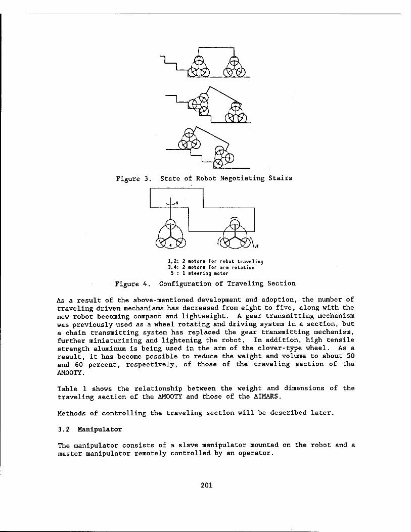
Figure 3. State of Robot Negotiating Stairs

1,2: 2 motors for robot traveling 3,4: 2 motors for arm rotation S : 1 steering motor

Figure 4. Configuration of Traveling Section

As a result of the above-mentioned development and adoption, the number of traveling driven mechanisms has decreased from eight to five, along with the new robot becoming compact and lightweight. A gear transmitting mechanism was previously used as a wheel rotating and driving system in a section, but a chain transmitting system has replaced the gear transmitting mechanism, further miniaturizing and lightening the robot. In addition, high tensile strength aluminum is being used in the arm of the clover-type wheel. As a result, it has become possible to reduce the weight and volume to about 50 and 60 percent, respectively, of those of the traveling section of the AMOOTY.

Table 1 shows the relationship between the weight and dimensions of the traveling section of the AMOOTY and those of the AIMARS.

Methods of controlling the traveling section will be described later.

3.2 Manipulator

The manipulator consists of a slave manipulator mounted on the robot and a master manipulator remotely controlled by an operator.

201

Table 1. Comparison Between Traveling Section of Intelligent Working Robot and That of System Maintaining Robot (AMOOTY)

Item Intelligent working robot

AMOOTY

Total weight (Weight of traveling section)

Overall length

Overall height

Overall width

Traveling performance Turning radius Stairs Speed Weight on board

220 kg (160 kg) 360 kg (300 kg)

1,650 mm

700 mm

700 mm

1,000 mm 30°, 150 m 1 km/hour

About 100 kg

1,600 mm

1,187 mm

740 mm

600 mm 35°, 220 mm 0.54 km/hour About 60 kg

The slave manipulator must be lightweight because it is mounted on the previously-mentioned traveling section. On the other hand, in order to carry out nonroutine and complex work, it is preferable that the robot have much freedom of movement and many articulations. It was decided that lightweight materials (for example, carbon fiber glass reinforced plastics [CFRP] is used in the external cylinder of the arm) would be used for the former, while the degree of freedom would be determined for the latter by analyzing the distribution of degrees of optimum freedom in order to satisfy the above contradictory conditions. As a result of studying this matter, it has become possible to realize a manipulator with 9 degrees of freedom of movement, an overall length of about 1.7m, and a dead load of about 61 kg. Figure 5 shows a block diagram of a manipulator consisting of an arm with 9 degrees of freedom of movement and four articulations, and a hand equipped with a force sensor. This manipulator employs a distribution system in which each articulation is equipped with a motor and a power transmitting mechanism (gear, etc.). Also, three kinds of controlling methods (mentioned later) are combined for the manipulator.

In addition, a microminiature charge coupled device [CCD] color camera is installed in the hand so that more detailed information on work targets can be given to an operator. Due to such information, the operator progress will increase. Figure 6 [not reproduced] illustrates a slave manipulator and a microminiature color CCD camera1* installed on the hand. Figure 7 [not reproduced] illustrates a master manipulator. This master manipulator is of a modified type, and has a scale of about two-thirds that of the slave manipulator.

202

Hand

2d articulation

1st articulation

4th articulation

Weight: about 61 kg Overall length: about 1,67B mm ■ Outside diameter: 13G mm (max) J Weight as a manipulator's I

capacity: about IB kg Freedom of movement: 9 ♦ hand

Figure 5. Configuration of Manipulator

3.3 Sensor Section and Control Section

Both manipulation control and traveling control, the main forms of comprehensive control, are generalized for this intelligent working robot so that various sensors can be combined and used with each other. The visual sensor for use in understanding environments, the ultrasonic sensor used mainly when the robot is traveling, the tilt angle gauge, etc., can be cited as some of the above various sensors. Figure 8 shows a block diagram of the robot's control system, and Table 2 shows specifications and the main uses of various sensors.

O Microminiature CCD color section

Manipulator

.Stereoscopic TV camera for distance Measurement

Stereoscopic TY caiera

Visual section

Universal head

Travelina section

Figure 8. Block Diagram of Control System of Intelligent Working Robot

Information for main control is input as images of the target and travel paths in an image processing unit [TOSPIX-II] by using a visual sensor. The object is recognized by processing the information, and the results of measuring the distance between the object and the robot is used.

203

Table 2. Sensors for Robot Traveling

Use

For autonomous traveling of robot

Visual sensor Otber sensors

Internal sensor External sensor

•Microminiature CCD »Traveling dis- »Ultrasonic color TV camera tance detecting sensor

sensor •Gyroscope

•Steering angle detecting sensor »Tilt angle

sensor •Arm angle detect- ing sensor »Photoelectric

sensor

•Stereoscopic TV camera for dis- tance measurement

(1) Comprehensive Control

The integrated control section comprehensively controls the entire system, makes plans for robot behavior based on the processing results obtained from the image processing unit, outputs operation commands for the traveling- section/universal head controller and a slave controller for manipulators, obtains operating states of the robot from each controller, and outputs these operating states to a display screen preparation unit. In addition to this integrated control system, the robot has operation input systems, such as an operation mode switch, joystick witch used to input data manually, etc. These operation input systems will be described in the next paragraph.

(2) Traveling Control

The autonomous traveling control perceives paths, walls, etc., with a visual sensor in accordance with the control flow shown in Figure 9, the information perceived with the visual sensor is processed with an image processing unit, TOSPIX-il, and the traveling section is autonomously induced by combining the results obtained by processing this information with information on the traveling path (map) submitted in advance. The control of the traveling section is broadly classified into two kinds, i.e. , flat traveling control and stair traveling control.

• Flat Traveling Control

When the robot travels on a straight section, it will detect a white line, which expresses the width of a path, with its microminiature CCD color camera, and will calculate the difference between the center of the robot and that of the path. That is, in such cases, it will autonomously travel on the path by using the algorithm. Figure 10 [not reproduced] shows an image example for the case in which the robot travels on a straight line processed with an image processing unit while catching a path, with a camera installed on the hand of the previously-mentioned manipulator.

204

C STAUT )

Figure 9. Flowchart of Autonomous Traveling Control

Also, when the robot traverses corners and negotiates stairs, visual information is combined with other information obtained from an ultrasonic sensor and a gyroscope. As a result, autonomous traveling control with higher reliability has been realized.

• Stair Traveling Control

As shown in Figure 3, the ascending and descending of stairs has been realized with an arm angle detecting sensor of the clover-type wheel and a tilt angle sensor of the robot and by adjusting and controlling the front and rear wheels.

(3) Manipulator Control

The following control system was adopted as a manipulator control. A work target is caught with two visual sensors, the distance between the robot and the object is measured by processing images of the object, and the manipulator is placed close to the object based on this distance-related data.

It was decided that an operator would remotely control the robot so that the robot could carry out complex and minute work, such as the final application of tools to an object, etc. For this reason, bilateral control has been realized, raising remote controllability, by installing a strain gauge and a force sensor on each section of the manipulator. The force sensor senses the gripping of an object, and transmits this sense to an operator.

As shown below, the manipulator control is classified into modes.

205

Autonomous mode: Images sent from a visual sensor (stereoscopic TV camera for measuring distance) are processed with an image processing unit, the coordinates of an object are found, and the manipulator is transferred in front of the object based on the results of the above processing and findings. (CP control)

Automatic mode: When there is no change in the relationship between the relative position of an object and that of the robot, even when the robot travels on a road, etc., (for example, tools on the robot), a task is instructed to the robot in advance, and the instruction is regenerated as necessary. (Teaching playback control)

Remote mode: An operator controls the master manipulator while monitoring the robot by using a TV camera for manipulators on the operation table and a stereoscopic TV camera, and makes the robot carry out work while driving the slave manipulator. (Master slave control)

The autonomous and automatic control of the manipulator with 9 degrees of freedoms of movement is divided into 3 degrees of freedom (SI, R2, P3) at the base side and 6 (R4, P5, P6, R7, P8, and R9) at the arm side,'a robot controller is installed in each side, mutual timing is secured, and the base and arm are driven simultaneously. The use of this method enables an operator to reduce the time involved and to make the robot carry out work smoothly. Figure 11 shows the autonomous control flow of the manipulator's work.

Top coordinate at the base side is calculated from coordinate values of an object obtained at the com- prehensive control section by using an image processing unit.

I

Top coordinate value at the base side and coordinate values of the object are transmitted to the base and arm controller.

I

Starting commands are sent, and base and arm are driven simultaneously.

Figure 11. Flowchart of Autonomous Control of Manipulator

3.4 Operation Input System and Indicator

This robot is designed so that simple work is autonomously or automatically controlled and complex work is remotely controlled by an operator on the basis of the operator's judgments. Therefore, the robot is configured so that the operator can readily handle the operation input system and indicator, and easily understood information is transmitted to the operator.

206

Three joystick switches are adopted in the remote controlled operation input system of the traveling section, and a master manipulator is used for manipulative work.

Figure 12 [not reproduced] shows the exterior of the operation input system and that of the manipulator. Even an operator can conduct operation input work. This operation input system is equipped with an image indicating section for a microminiature CCD color stereoscopic TV camera mounted on the robot so that the operator can handle the manipulator while watching images. In addition, a three-dimensional color graphic indicator is adopted in the system to clearly transmit states of the robot to the operator. This indicator shows such states as three-dimensional animations at real time. Figure 13 [not reproduced] shows an example of a three-dimensional animation indicated by combining the tested unit and the robot.

4. System Test and Result

The tester shown in Figure 14 was made, and tests of the following two items were conducted to grasp the performance of the intelligent working robot we developed:

1) Autonomous traveling test 2) Manipulation test

(1) Autonomous Traveling Test

A traveling test was conducted on a traveling path with an overall length of about 14 m, as shown in Figure 14. It was confirmed that the robot could autonomously travel on the traveling sections, such as straight sections, corners, and stairs (tilt angle of 30 degrees and step height of 150 mm), in accordance with the control flow shown in Figure 9, by combining such sensors as visual sensors, ultrasonic sensors, gyroscopes, and tilt angle gauges. Also, no problems occurred when handling a flange bolt of a tank after the robot stopped at the end point of a traveling section because the stop position accuracy of the robot was very high.

(2) Manipulation Test

It was confirmed that the operator could remotely control the work involved in increasingly tightening the flange bolt (M 24) about 1 m in front of the end point from the master manipulator by using a ratchet-type tool, as shown in Figure 15 [not reproduced], while watching the color stereoscopic TV screen. Figure 16 [not reproduced] shows the remote control in progress.

When the operator remotely controls all of the manipulative work, his burden will be extremely heavy. Accordingly, as previously mentioned,this robot employs a method in which the manipulator is automatically or autonomously controlled and placed close to an object based on the distance information obtained from image information sent from the visual sensor.

As a result of conducting the above tests, it has been confirmed that the use of this method will decrease the burden on the operators.

207

Traveling * path (white .2 line)

Wall

Stairs

J^End point

Working floor

Figure 14. Tester Configuration for Intelligent Working Robot

5. Conclusion

As mentioned previously, we have developed the AIMARS, and have grasped its basic performance. We are currently continuing tests and studies of a cableless robot, and are planning to improve the AIMARS functions further.

Also, the AIMARS is somewhat limited by environmental conditions when use of the visual sensor is involved. On the other hand, however, with regard to "Robot Engaged in Very Dangerous Environments" being developed as a significant project by the AIST, we have developed a visual information processing technology which can be used to recognize object, such as valves and pumps, in very complex environments in nuclear power plants.1,15"16 The AIST is scheduled to complete this project by FY 1990. We are scheduled to fully utilize the above technology in the AIMARS, to expand the locomotion and working ranges of the robot, and to put the robot close to practical use in the future.

References

1. Tatsuo Miyazawa, et al., "Development of Robot in Nuclear Power--New Stage of Intelligent Robot," NUCLEAR INDUSTRY, Vol 34 No 4, 1988, pp 7-33.

2. Ryouichi Nakayama, et al., "Development of Half-Moon Type Crawler Vehicle Used in Nuclear Inspection Robots," JAPAN ROBOT ASSOCIATION JOURNAL, Vol 2 No 3, 1984, pp 238-243.

3. Ibid., "Development of System for Automatically Inspecting Inside of Reactor Containers," Japan Machinery Association Lecture Papers No 860-1 (The 14th Technical Lecture Meeting/Up-to-Date Application Technology for Factory Automation [FA] and Robot), 1986, pp 33-36.

4. Ibid., "Development of Nuclear Inspecting Robot--Application of Floor Traveling Vehicle," Japan Robot Association, et al., the 3d Intelligent Locomotive Robot Symposium, 1986, pp 115-120.

208

5. Hiroaki Andoh, "Research and Development of Working Robot in Practical Nuclear Power Generating Facilities," ENERGY AND RESOURCE, Vol 8 No 2, 1986, pp 165-170.

6. Shinobu Sagisawa, "Tendency for Research and Development of Robots Engaged in Very Dangerous Environments," TECHNOLOGY FOR AUTOMATION, Vol 20 No 1, 1988, pp 15-1.

7. Tatsuo Miyazawa, et al. , "Intelligence of Nuclear Power Plant Inspecting and Monitoring Robot," JOURNAL OF ATOMIC ENERGY SOCIETY OF JAPAN [JAES], Vol 28 No 11, 1986, pp 994-1002.

8. Katsuhiko Satoh, et al., "Development of System Maintaining Robot, AMOOTY," Japan Machinery Association Lecture Papers, No 860-1 (The 14th Technical Lecture Meeting/Up-to-Date Application Technology for FA and Robot), 1986, pp 37-40.

9. Tatsuo Miyazawa, et al. , "Intelligent Working Robot in Nuclear Field," Japan Radioisotope Association [JRIA], ISOTOPE NEWS, July 1987, PP 2-7.

10. Ryouichi Nakayama, etal., "Development of Intelligent Working Robot, " JAPAN ROBOT ASSOCIATION JOURNAL, Vol 5 No 5, 1987, pp 81-86.

11. Ibid., "Robot Technology for Nuclear Power," TOSHIBA REVIEW, Vol 43 No 1, 1988, pp 27-30.

12. Ibid., "Robot for Toshiba Corporation's Nuclear Power," Toshiba Japan Machinery Association Lecture Papers, 1987, No 870-10, pp 226-229.

13. Hideharu Okano, et al., "Locomotive Intelligent Robot for Inspection and Maintenance of Nuclear Power Plants," ELECTRIC ASSOCIATION JOURNAL, 1987, pp 22-26.

14. Hiroo Takemura, et al., "Microminiature CCD Camera," TOSHIBA REVIEW, Vol 41 No 6, 1986, pp 539-542.

15. Yoshitoku Kuno, et al., "Application of Robot Vision to Nuclear Power Plants," Ibid., Vol 41 No 1, 1986, pp 75-78.

16. Hiroshi Hoshino, "Visual Sense of Robot for Nuclear Power Generating Plants," TELEVISION ASSOCIATION JOURNAL, Vol 41 No 10, 1987, pp 954-958.

- END -

209