1 physical principles of evolution

1

Physical principles of evolution

Peter Schuster

Institut fur Theoretische Chemie der Universitat Wien, Wahringerstraße 17,1090 Wien, Austria, pks @ tbi.univie.ac.at

Abstract. Theoretical biology without a comprehensive theory of evolution is in-complete, since evolution is in the core of biological thought. Evolution is visualizedas a migration process in genotype or sequence space that is either an adaptivewalk driven by some fitness gradient or a random walk in absence of (sufficientlylarge) fitness differences. The Darwinian concept of natural selection consisting inthe interplay of variation and selection is based on a dichotomy: All variations occuron genotypes whereas selection is operating on phenotypes and relations betweengenotypes and phenotypes as encapsulated in a mapping form genotype space intophenotype space are central for an understanding of evolution. Fitness is conceived asa function of the phenotype represented by a second map from phenotype space intononnegative real numbers. In the biology of organisms, genotype-phenotype mapsare enormously complex and relevant information on them is exceedingly scarce. Thesituation is better in the case of viruses but so far only one example of a genotype-phenotype map, the mapping of RNA sequences into RNA secondary structures,has been investigated in sufficient detail. It provides direct information of RNAselection in vitro and test-tube evolution, and it is a basis for testing in silico evo-lution on a realistic fitness landscape. Most of the modeling efforts in theoreticaland mathematical biology of today are done by means of differential equations butstochastic effects are of undeniably great importance for evolution. Population sizesare much smaller than the numbers of genotypes constituting sequence space. Everymutant, after all, has to begin with a single copy. Evolution can be modeled by achemical master equation, which (in principle) can be approximated by a stochas-tic differential equation. In addition, simulation tools are available that computetrajectories for master equations. The accessible population sizes in the range of107 ≤ N ≤ 108 molecules are commonly too small for problems in chemistry butsufficient for biology.

1.1 Mathematics and biology

The beginning of modern science in the sixteenth century has been initi-ated by the extremely fruitful marriage between physics and mathematics.Nobody has expressed the close relation between mathematics and physics

2 Peter Schuster

clearer than Galileo Galilei in his famous statement [1]: Philosophy (science)is written in this grand book, the universe, .... . It is written in the languageof mathematics, and its characters are triangles, circles and other geometricfeatures. ... . Indeed, physics and mathematics have cross-fertilized each otherfrom the beginnings of modern science until present day. Theoretical physicsand mathematical physics are highly respected disciplines and no physics jour-nal will accept empirical observations without an attempt to bring it into acontext that allows for quantification and interpretation by theory. Generalconcepts and successful abstractions have a high reputation in physics and thereductionists’ program1 is the accepted scientific approach towards complexsystems. This view is common in almost all subdisciplines of contemporaryphysics and, in essence, is shared with chemistry and molecular biology.

Conventional biology, in this context, is very different: Great works ofbiology like Charles Darwin’s Origin of Species [2] or in recent years ErnstMayr’s Growth of Biological Thought [3] do not contain a single mathemat-ical expression, theoretical and mathematical biology had and still have abad reputation among macroscopic biologists, special cases are preferred overgeneralizations, which are looked upon with scepticism, and holistic viewsare commonly more appreciated than reductionists’ explanations no matterwhether they are in a position to provide insight into problems or not. Afamous and unique exception among others is Charles Darwin’s theory of nat-ural selection by reproduction and variation in finite populations. Althoughnot cast into mathematical equations, the theory is based on a general conceptwhose plausibility is erected upon a wealth of collected and carefully inter-preted empirical observations. Darwin’s strategy has something in commonwith the conventional mathematical approach based on observation, abstrac-tion, conjecture, and proof: On different islands of the Galapagos archipelagoDarwin observed similar looking species in different habitats and concludedcorrectly that these different species are closely related and owe their existenceto histories of adaptation to different environments on the individual islands.The occurrence of adaptations has been attributed to natural selection as acommon mechanism through abstraction from specific cases. Darwin’s conjec-ture combines three facts known at his times:

(i) Multiplication: All organisms multiply by cell division, parthenogenesisor sexual reproduction, multiplication is accompanied by inheritance –

1 The reductionist program, also called methodological reductionism, aims at anexploration of complex objects through breaking them up into modular, preferen-tially molecular parts and studying the parts in isolation before reassembling theobject. Emergent properties are assumed to be describable in terms of the phe-nomena from and the processes by which they emerge. The reductionist programis different from ontological reductionism, which denies the idea of ontologicalemergence by the claim that emergence is merely a result of the system’s descrip-tion and does not exist on a fundamental level.

1 Physics of evolution 3

’progeny resembles parents’, and under the condition of unlimited re-sources multiplication results in exponential growth of population size.

(ii) Variation: All natural populations show variance in phenotypic proper-ties either continuously varying features like body size or discontinuouslyvarying features like the number of limbs, the number of digits, color offlowers, skin patterns or seeds shapes, and it is straightforward to relatevariation to inheritance.2

(iii) Selection: Exponential growth results in overpopulation of habitats,3

only a small fraction of offspring can survive and have progeny of theirown, and this stringent competition prevents less efficient variants fromreproduction.

Taking together the three items and introducing the notion of fitness for thenumber of offspring, which reach the age of fertility, the conjecture could beformulated in the following way:

Natural selection: In nonhomogeneous populations the frequenciesof variants with fitness values below the population average are de-creasing, those with fitness values above average are increasing andconsequently the population average itself will increase until it reachesthe maximum value corresponding to a homogeneous population of thebest adapted or fittest variant.

Darwin’s Origin of Species is an overwhelming collection of observations fromnature, from animal breeders and from nursery gardens that provide strongevidence for the correctness of Darwin’s conjecture. This enormous collectionin a way is the empirical substitute for a mathematical proof.

Although Gregor Mendel analyzed his experiments on inheritance in peasby mathematical statistics and found thereby the explanatory regularities,mathematics did not become popular in biology. In contrary, Mendel’s workhas been largely ignored by the biological community for more than thirtyyears. Then, Mendel has been rediscovered and genetics became an impor-tant discipline of biology. Population genetics has been founded by the threescholars Ronald Fisher [8], J.B.S. Haldane [9] and Sewall Wright [10]. In thenineteen thirties they succeeded to unite Mendelian genetics and Darwin’snatural selection, and to cast evolution into a rigorous mathematical framebut conventional geneticists and evolutionary biologists continued to fight un-til the completion of the synthetic theory almost twenty years later [3].

2 Gregor Mendel was the first to investigate such relations experimentally [4–6] anddiscovered the transmittance of properties in discrete packages from the parentsto offspring. His research objects were the pea (pisum) from where he derived hisrules of inheritance and the hawkweed (hieracium), which was rather confusingfor him, because it is apomictic, i.e. it reproduces asexually. Charles Darwin,on the other hand, had a mechanism of inheritance in mind, which was entirelywrong. It was based on the idea of blending of the parents’ properties,

3 According to his own records Charles Darwin has been influenced strongly byRobert Malthus and his demographic theory of [7].

4 Peter Schuster

Modeling in biology became an important tool for understanding com-plex dynamical phenomena. Representative for many other approaches wemention here only three: (i) Modeling of coevolution in a predator-prey sys-tem was introduced by Alfred Lotka [11] and Vito Volterra [12] by meansof differential equations that were borrowed from chemical kinetics. In a way,they were the pioneers of theoretical ecology, which has been developed by thebrothers Howard and Eugene Odum [13] and became a respectable field of ap-plied mathematics later [14]. (ii) A model for pattern formation based on thereaction-diffusion (partial differential) equation with a special chemical mech-anism has been suggested and analyzed by Alan Turing [15]. Twenty yearslater the Turing model was applied to biological morphogenesis [16, 17] andprovided explanations for patterns formed during development [18, 19]. (iii)Based on experimental studies of nerve pulse propagation in the squid giantaxon Alan Hodgkin and Andrew Huxley formulated a mathematical model fornerve excitation and pulse propagation [20] that became the standard modelfor single nerve dynamics in neurobiology. They both were awarded the NobelPrize in Medicine in 1963. A second breakthrough in understanding neuralsystems came from modeling networks of neurons. John Hopfield conceivedan exceedingly simple model of neurons in networks [21] that initiated a wholenew area of scientific computing: computation with neural networks , in partic-ular modeling and optimization of complex systems. Despite these undeniableand apparent successes, the scepticism of biologists with respect to theoryand mathematics, nevertheless, continued for almost the entire rest of thetwentieth century.

The advent of molecular biology in the nineteen fifties brought biologycloser to chemistry and physics, and changed the general understanding ofnature in a dramatic way [22]. Inheritance got a profound basis in molecu-lar genetics and reconstruction of phylogenies became possible through com-parison of biopolymer sequences from present day organisms. Structures ofbiomolecules at atomic resolution were determined by refined techniques fromphysical chemistry and they gave deep insights into biomolecular functions.Spectroscopic techniques, in particular nuclear magnetic resonance, require asolid background in mathematics and physics for conceiving and analyzingconclusive experiments. A novel era of biology was initiated in the nineteenseventieth when the highly efficient new methods for DNA sequencing de-veloped by Walter Gilbert and Frederick Sanger became available [23, 24].Sequencing whole genomes became technically within reach and financiallyaffordable. The first two complete bacterial genomes were published in 1995[25] and the following years saw a true explosion of sequencing data. High-throughput techniques using chip technology for genome wide analysis oftranslation and transcription products known as proteomics and transcrip-tomics followed and an amount of data was created that has never been seenbefore. In this context it is worth to cite the Nobel laureate Sydney Bren-ner [26] who made the following statement in 2002 to characterize the situationin molecular biology:


“I was taught in the pre-genomic era to be a hunter. I learnt how toidentify the wild beasts and how to go out, hunt them down and killthem. We are now, however, being urged to be gatherer. To collecteverything lying about and and put it into storehouses. Someday, it isassumed someone will come and sort through the storehouses, discardthe junk and keep the rare finds. The only difficulty is how to recognizethem.”

Who else but a theorist should be this “someone”? The current developmentseems to indicate that “someday” is not too far away. The flood of data andthe urgent need for a comprehensive theory have driven back the aversionfor computer science and mathematics of the biologists. Modern genetics andgenome analysis without bioinformatics are unthinkable and understandingnetwork dynamics without mathematics and computer modeling is impossible.

The new discipline of systems biology has the ambitious goal to find holisticdescriptions for cells and organisms without giving up the roots in chemistryand physics. Although still in its infancy and falling into one trap after an-other, modeling in systems biology progresses slowly towards larger and moredetailed models for regulatory modules in cell biology. New techniques are de-veloped and applied, examples are flux-balance analysis [27] and applicationof inverse methods [28], whereby the primary challenge is up-scaling to largersystems like whole organisms. Recent advances in experimental evolution al-low for an extension of detailed models to questions of evolution, which is ofcentral importance of biology as Theodosius Dobzhansky has encapsulated inhis famous sentence: “Nothing in biology makes sense except in the light ofevolution” [29]. From a conceptional point of view, theoretical biology is in abetter position than theoretical physics where the attempts of unification ofthe two fundamental theories, quantum mechanics and relativity theory, havenot been successful so far. Biology has one comprehensive theory, the the-ory of evolution, and present day molecular biology is building the bridge tochemistry and physics. Missing are a proper language and efficient techniquesto handle the enormous complexity and to build proper models.

1.2 Darwin’s theory in mathematical language

If Charles Darwin would have been a mathematician, how might he haveformulated his theory of natural selection? Application of mathematics toproblems in biology has a long history. The first example that is relevant forevolution dates back to medieval times. In the famous Liber Abaci written inthe year 1202 by Leonardo Pisano also known as Fibonacci (filius Bonacci)we find a counting example of the numbers of pairs of rabbits in subsequenttime spans. Every adult pair is assumed to give birth to another pair, newborn rabbits have to wait one time interval before they become fertile adults.Starting from a single couple yields the following series:

(0) 1 1 2 3 5 8 13 21 34 55 89 . . . .

6 Peter Schuster

Time t

Popula

tion v

ariable

( )

,x

ty

t( )

Fig. 1.1. Fibonacci series, exponential functions, and limited resources.The Fibonacci series (black; upper plot) is embedded between two exponentialfunctions in the range 0 < i ≤ 10: nupper(t) = exp

(

0.4453 · (t − 1))

(red) andnlower(t) = exp

(

0.5009 · (t− 2))

(blue), wherein the time t is the continuous equiv-alent to the discrete (generation) index i. The lower plot compares the exponentialfunction, y(t) = y0 exp(r t) for unlimited growth (red; y0 = 0.02, r = 0.1) with thenormalized solution of the Verhulst equation (x(t), black; x0 = 0.02, r = 0.1, andC = 1 by definition)

Every number is the sum of its two precursors and the Fibonacci series isdefined by the recursion

Fi+1 = Fi + Fi−1 with F0 = 0 and F1 = 1 . (1.1)

It is straight forward to show that the Fibonacci series can be approximatedwell by exponential functions as upper and lower limits (Fig. 1.1). The expo-nential function, however, was not known before the middle of the eighteenth


century, it was introduced in the fundamental work of the Swiss mathemati-cian Leonhard Euler [30]. Robert Malthus – although living fifty years later– still uses a geometric progression, 2, 4, 8, 16, . . . , for the unlimited growthof populations [7]. The consequences of unlimited growth for demography aredisastrous and, as said, Malthus’ work was influential on Darwin’s thoughts.

A contemporary of Charles Darwin, the mathematician Pierre-FrancoisVerhulst [31], formulated a model based on differential equations combiningexponential growth and limited resources (Fig. 1.1):

dN

dt= N = r N

(

1 − N

C

)

(1.2)

with N(t) describing the number of individuals at time t, r being the Malthu-sian parameter and C the carrying capacity of the ecosystem. Equ. (1.2) con-sists of two terms: (i) the exponential growth term, rN , and (ii) the constraintto finite population size expressed by the term −rN2/C. In other words, theecosystem can only support N = C individuals and limt→∞N(t) = C. Thesolution of the differential equation (1.2) is of the form

N(t) =N0 C

N0 + (C −N0) exp(−rt) . (1.3)

Herein N0 = N(0) is the initial number of individuals. It its straightforwardto normalize the variable to the carrying capacity, x(t) = N(t)/C yielding

x(t) =x0

x0 + (1 − x0) exp(−rt) (1.3’)

with x0 = N0/C. It will turn out to be useful to cast the term representing theconstraint into the form N φ(t)/C = xφ(t). Then, we obtain for the Verhulstequation

dx

dt= x = x

(

r − φ(t))

with φ(t) = x r (1.2’)

being the (mean) reproduction rate of the population.Eventually, we generalize to the evolution of n species or variants4 in

the population Ξ = {X1, X2, . . . , Xn}. The numbers of individuals are nowdenoted by [Xi] = Ni with

∑ni=1Ni = N and the normalized variables

xi = Ni/N with∑n

i=1 xi = 1. Each variant has its individual Malthus param-eter of fitness value fi, and for the selection constraint leading to constantpopulation size we find now φ(t) =

∑ni=1 xi fi, which is the mean reproduc-

tion rate of the entire population. The selection constraint φ(t) can be usedfor modeling much more general situations than constant population size by

4 In this chapter we shall not consider sexual reproduction or other forms of re-combination. In asexual reproduction a strict distinction between variants andspecies is neither required nor possible. We shall briefly come back to the prob-lem of bacterial or viral species in section 1.7.

8 Peter Schuster

means of the mean reproduction rate. As we shall see in section 1.5, the prooffor the occurrence of selection can be extended to very general selection con-straints φ(t) as long as the population size does not become zero, N > 0.

The kinetic differential equation in the multi-species case, denoted as se-lection equation,

xj = xj

(

fj − xj

n∑

i=1

xi fi

)

= xj

(

fj − xj φ(t))

, j = 1, 2, . . . , n , (1.4)

can be solved exactly by the integrating factors transform ([32], p.322ff.)

zj(t) = xj(t) · exp

(∫ t

0

φ(τ)dτ

)

. (1.5)

Insertion into (1.4) yields

zj = fjzj and zj(t) = zj(0) · exp(fjt) ,

xj(t) = xj(0) · exp(fjt) · exp

(

−∫ t

0

φ(τ)dτ

)

with

exp

(∫ t

0

φ(τ)dτ

)

=

n∑

i=1

xi(0) · exp(fit) ,

where we have used zj(0) = xj(0) and the condition∑n

i=1 xi = 1. The solutionfinally is of the form

xj(t) =xj(0) · exp(fjt)

∑ni=1 xi(0) · exp(fit)

; j = 1, 2, . . . , n . (1.6)

The interpretation is straightforward. The term with the largest fitness value,fm = max{f1, f2, . . . , fn}, dominates the sum in the denominator after suffi-ciently long time:5

n∑

i=1

xi(0) · exp(fit) → xm(0) · exp(fmt) for large t and xm(t) → 1 .

Optimization in the sense of Charles Darwin’s principle of selection of thefittest variant, Xm, takes place.

The occurrence of selection in equ.(1.4) can be verified also without know-ing the solution (1.6). For this goal we consider the time dependence of theconstraint φ, which is given by

5 We assume here that the largest fitness value fm is non-degenerate, i.e. there isno second species having the same (largest) fitness value. In section 1.5 we shalldrop this restriction.


0

421 8 16

10

19

9

14

6

13

5

11

3

7

12

21

17

22

18

25

20

26

24

28

272315 29 30

31

Mutant class

0

1

2

3

4

5

Fig. 1.2. Sequence space of binary sequences of chain length ℓ = 5. Thesequence space Q{0,1}

5 comprises 32 sequences. Every sequence is represented bya point. The numbers in the yellow balls are the decimal equivalents of the bi-nary sequences and can be interpreted as sequences of two nucleotides, “0”≡ “C”and “1”≡ “G”. Examples are 0≡ 00000≡CCCCC, 14≡01110≡CGGGC or 29≡11101≡GGGCG. All positions of a (binary) sequence space are equivalent in thesense that each sequence has ℓ nearest neighbors, ℓ(ℓ − 1)/2 next nearest neigh-bors, etc. Accordingly, sequences are properly grouped in mutant classes around thereference sequence, here 0.

dφ

dt=

n∑

i=1

fixi =

n∑

i=1

fi

(

fixi − xi

n∑

j=1

fjxj

)

=

=n∑

i=1

f2i xi −

n∑

i=1

fixi

n∑

j=1

fjxj =

= f2 −(

f)2

= var{f} ≥ 0 . (1.7)

Since a variance is always nonnegative, equ.(1.7) implies that φ(t) is a non-decreasing function of time. The value var{f} = 0 implies a (local) maximumof φ and hence, φ is optimized during selection. Zero variance is tantamountto a homogeneous population containing only one variant. Since φ is at amaximum, this is the fittest variant Xm.

10 Peter Schuster

1.3 Evolution in genotype space

Evolution can be visualized as a process in an abstract genotype or sequencespace, Q. At constant chain lengths ℓ of polynucleotides the sequence space isspecified as QA

ℓ were A is the alphabet, for example A = {0, 1} or A = {G,C}is the binary alphabet and A = {A,U,G,C} the natural nucleotide alphabet.The gain of such a comprehensive view of genotypes is generality and the framefor reduction to the essential features, the shortcomings, obviously, are lack ofdetail. Building a model for evolution upon a space that fulfils all requirementsrequired for the molecular view of biology and which may, eventually, bridgemicroscopic and macroscopic views, is precisely what we are aiming for here.The genotypes are DNA or RNA sequences and the proper genotype spaceis sequence space. The concept of a static sequence space [33, 34] has beeninvented in the early nineteen seventieth in order to bring some ordering cri-teria into the enormous diversity of possible biopolymer sequences. Sequencespace QA

ℓ as long we are only dealing with reproduction and mutation is ametric space with the Hamming distance6 serving as the most useful metricfor all practical purposes. Every possible sequence is a point in the discretesequence space and in order to illustrate the space by a graph, sequencesare represented by nodes and all pairs of sequences with Hamming distanceone by edges (Fig. 1.2 shows a space of binary sequences as an example. Bi-nary sequence spaces are hypercubes of dimension ℓ being the length of thesequences).

Two properties of sequence spaces are important: (i) All nodes in a se-quence space are equivalent in the sense that every sequence has the samenumber of nearest neighbors with Hamming distance dH = 1, next nearestneighbors with Hamming distance dH = 2, and so on, which are grouped prop-erly in mutant classes. (ii) All nodes of a sequence space are at the boundary ofthe space or, in other words, there is no interior. Both features are visualizedeasily by means of hypercubes:7 All points are positioned at equal distancesfrom the origin of the (Cartesian) coordinate system. What makes sequencespaces difficult to handle are neither internal structures nor construction prin-

6 The Hamming distance dH(Xi, Xj) [35] counts the number of positions at whichtwo aligned sequences Xi and Xj differ. It fulfils the four criteria for a metric insequence space: (i) dH(Xi, Xj) ≥ 0 (non-negativity), (ii) dH(Xi, Xji) = 0 if anonly if Xi = Xj (identity of indiscernibles), (iii) dH(Xi, Xj) = dH(Xi, Xj) (sym-metry), and (iv) dH(Xi, Xj) ≤ dH(Xi, Xk)+dH(Xi, Xk) (triangle inequality). Forsequences of equal chain length ℓ end-to-end alignment is the most straightfor-ward alignment, although it may miss close relatedness that is a consequence ofdeletions and insertions, which are mutations that alter sequence length.

7 An ℓ-dimensional hypercube in the Cartesian space of dimension ℓ is the analogueof a (three-dimensional) cube. The ℓ-dimensional hypercube is constructed bydrawing 2ℓ (hyper)planes of dimension (ℓ − 1) perpendicular to the coordinateaxes at the positions ±a. The corners of the hypercubes are the 2ℓ points whereℓ planes cross.


ciples but the hyper-astronomically large numbers of points: |QAℓ | = κℓ for

the sequences of length ℓ over an alphabet of size κ with κ = |A|.The population Ξ = {X1, X2, . . . , Xn} is represented by a vector with the

numbers of species as elements N = (N1, N2, . . . , Nn), the population size isthe L1-norm:

N = ‖N‖1 =n∑

i=1

|Ni| =n∑

i=1

Ni ,

where absolute values are dispensable since particle numbers are real and non-negative by definition. Normalization of the variables yields x = N/‖N‖ orxi = Ni/N and

∑ni=1 xi = 1, respectively. A population is thus represented

by an L1-normalized vector x and the population size N . An important prop-erty of a population is its consensus sequence, X, consisting of a nucleotidedistribution at each position of the sequence. This consensus sequence can bevisualized as the center of the population in sequence space.

A sequence is conventionally understood as a string of ℓ symbols chosenfrom some predefined alphabet with κ letters, which can be written as

Xj =(

b(j)1 , b

(j)2 , . . . , b

(j)ℓ

)

with b(j)i ∈ A = {α1, . . . , ακ} .

The natural nucleotide alphabet contains four letters: A = {A,U,G,C}, butRNA molecules with catalytic functions have been derived also from three- andtwo-letter alphabets [36,37]. For the forthcoming considerations it is straight-forward to adopt slightly different definitions: A sequence Xj results from themultiplication of the alphabet vector α = (α1, . . . , ακ) with a κ× ℓ matrix Xj

having only 0 and 1 as entries:

Xj = α · Xj = α ·(

β(j)1 ,β

(j)2 , . . . ,β

(j)ℓ

)

with

β(j)i ∈

{

10...0

,

01...0

, . . . ,

00...1

}

.(1.8)

In other words, the individual nucleotides in the sequence Xj are replaced by

products of two vectors, b(j)i = α · β(j)

i .With the definition (1.8) it is straightforward to compute the consensus

sequence of a population Ξk:

Ξk = α ·n∑

j=1

x(k)j Xj , (1.9)

and the distribution of nucleotides at position “i” is given by

b(k)i = α ·

n∑

j=1

x(k)j β

(j)i . (1.9’)

12 Peter Schuster

It is important to note the difference between b(j)i and b

(k)i : The former refers

to the nucleotide at position “i” in a given sequence whereas the latter de-scribes the nucleotide distribution at position “i” in the population. In caseone nucleotide is dominating at every position the distribution can be col-lapsed to a single sequence, the consensus sequence.

The internal structure of every sequence space QAℓ is induced by point

mutation and this is essential for inheritance because it creates a hierarchy inthe accessability of genotypes. Suppose we have a probability p to make oneerror in the reproduction of a sequence then, provided mutation at differentpositions is assumed to be independent, the probability to make two errorsis p2, to make three errors is p3, etc. Inheritance requires sufficient accuracyof reproduction – otherwise children would not resemble their parents – andthis implies p has to be sufficiently small. Then, p2 is smaller and the powerseries p dH decreases further with increasing distance from the reference se-quence. This ordering of sequences according to a probability criterion thatis intimately related to the Hamming metric (see section 1.5). As a matter offact mutation is indeed a fairly rare event in evolution and populations arecommonly dominated by a well-defined single consensus sequence since singlenucleotide exchanges that occur at many different positions do not contributesignificantly to the average.

Evolutionary dynamics is understood as change of the population vectorsin time: N(t) or x(t). This change can be modeled by means of differentialequations (section 1.5) or stochastic processes (section 1.6). A practical prob-lem concerns the representation of genotype space. Complete sequence space,QA

ℓ has the advantage to cover all possible genotypes but its extension ishuge and, since the numbers of possible genotypes exceed all even the largestpopulations by far we are confronted with the problem that most degrees offreedom are empty and very likely will never be populated during the evo-lutionary process described. Alternatively the description could be restrictedto those genotypes, which are actually present in the population and whichconstitute the population support Φ(t) that is defined by

Φ(t).= {Xj |Nj(t) ≥ 1} . (1.10)

The obvious advantage is a drastic reduction in the degrees of freedom to atractable size but one has to pay the price for the simplification: The pop-ulation support is time dependent and changes whenever a new genotype isproduced by mutation or an existing one goes extinct [38]. Depending on pop-ulation size population dynamics on the support can be described either bydifferential equations or modeled as a stochastic process. Support dynamics,on the other hand, is intrinsically stochastic since every mutant starts from asingle copy.

Finally, it is important to mention that recombination without mutationcan be modeled successfully as a process in an abstract recombination space[39–41] and plays a major role in the theory of genetic algorithms [42, 43].A great challenge for theorists is the development of a genotype space for


both, mutation and recombination. Similarly, convenient sequence spaces forgenotypes with variable chain lengths are not at hand.

1.4 Modeling genotype-phenotype mappings

Unfolding genotypes to yield phenotypes is studied in developmental biologyand provides the key to understanding evolution and, in particular, the originof species. For a long time it has been common knowledge already that thesame genotype can develop into different phenotypes depending on differencesin the environmental conditions and epigenetic effects.8 Current molecularbiology provides explanations for several epigenetic observations and revealsmechanisms for the inheritance of properties that are not encoded by the DNAof the individual. Still, genetics is shaping the phenotypes – otherwise progenywould not resemble parents – but epigenetics and environmental influencesprovide additional effects that are indispensable for understanding and mod-eling the relations between genotypes and phenotypes. Here we shall adoptthe conventional strategy of physicists and consider simple cases in whichthe genotypes unfolds unambiguously into a unique phenotype. This condi-tion is fulfilled, for example, in evolution in vitro when biopolymer sequencesform (the uniquely defined) minimum free energy structures as phenotypes.Bacteria in constant environments provide other cases of simple genotype-phenotype mappings (the long-term experiments of Richard Lenski [44–46]may serve as examples; see section 1.6). Under this simplifying assumptiongenotype-phenotype relations can be modeled as mappings from an abstractgenotype space into a space of phenotypes or shapes. A counter example ina simple system is provided by biopolymers with metastable suboptimal con-formations, which can serve a models where a single genotype – a sequence –can give rise to several phenotypes being molecular structures [47].

Since only point mutations shall be considered here, the choice of an appro-priate genotype space is straightforward. It is the sequence space QA

ℓ with theHamming distance dH as metric. The phenotype space or shape space Sℓ is thespace of all phenotypes formed by all genotypes of chain length ℓ. Althoughthe definition of a physically or biologically meaningful distance between phe-notypes is not at all straightforward, some kind of metric can always be found.Accordingly the genotype-phenotype mapping ψ can be characterized by

ψ :{

Q(A)ℓ ; dH(Xi, Xj)

} mfe===⇒ {Sℓ; dS(Si, Sj)} or Sk = ψ(Xk) . (1.11)

The map ψ need not be invertible. In other words, several genotypes canbe mapped onto the same phenotype when we are dealing with a case ofneutrality.

8 Epigenetics was used as a term subsuming phenomena that could not be explainedby conventional genetics.

14 Peter Schuster

-26.0

-24.0

-22.0

-20.0

-18.0

-16.0

-14.0

-12.0

-10.0

- 8.0

- 6.0

DG

[k

ca

l.m

ole

]-1

S0

S2

S3

S7,8

S9

2

3

87

9S10

S6S4,5

456

10

Kinetic structuresSuboptimal structuresMinimum free energy structure

S0

S1

S0S1

GGCCCCUUUGGGGGCCAGACCCCUAAAGGGGUC

Fig. 1.3. Secondary structures of ribonucleic acid molecules (RNAs). Con-ventional RNA folding algorithms compute the minimum free energy (mfe) struc-ture for a given sequence [48,49]. Hairpin formation is shown as an example on thel.h.s. of the figure. In addition, the sequence can fold also into a large number ofsuboptimal conformations (diagram in the middle of the figure), which are readilycomputed by efficient computer programs [50,51]. In case a suboptimal structure isseparated from the mfe-structure by a sufficiently high activation barrier, the struc-ture is metastable. The metastable structure in the example shown here is a doublehairpin (r.h.s. of the figure). The activation energy of more than 20 kcal/mole doesnot allow for interconversion of the two structures at room temperature (For thecalculation of kinetic structures see, for example, [52,53]).

An example of a genotype-phenotype mapping that can be handledstraightforwardly by analytical tools is provided by in vitro evolution of RNAmolecules [54–56]. RNA molecules are transferred to a solution containingactivated monomers as well as a virus-specific RNA replicase. The materialconsumed by the replication reaction is replenished by serial transfer of asmall sample into fresh solution. The replicating ensemble of RNA moleculesoptimizes the mean RNA replication rate of the population in the sense ofDarwinian evolution (see equ. 1.6). The interpretation of RNA evolution invitro identifies the RNA sequence with the genotype. The RNA structure, thephenotype, is responsible for binding to the enzyme and for the progress ofreproduction, since the structure of the template molecules has to opened inorder to allow for replication [57–59]. In case of RNA aptamer selection9 thebinding affinity is a function of molecular structure and sequence-structuremapping is an excellent model for the relation between genotype and pheno-type.

9 An aptamer is a molecule that binds to a predefined target molecule. Aptamersare commonly produced by an evolutionary selection process [60].


GGCCCCUUUGGGGGCCAGACCCCUAAAGGGGUCCCCA

GGCCCCUUUGGGGGCCAGACCCCUAAAGGGGUCCCCA

((((((((((((((.....))))))))))))))....

((((((....)))))).((((((....))))))....

5 -end‘

3 -end‘

5 -end‘

3 -end‘

Fig. 1.4. Symbolic notation of RNA secondary structures. RNA moleculeshave two chemically different ends, the 5’- and the 3’-end. A general conventiondetermines that all strings corresponding to RNA molecules (sequences, symbolicnotation, etc) start from the 5’-end and have the 3’-end at the r.h.s. The symbolicnotation is equivalent to graphical representation of secondary structures. Base pairsare denoted by parentheses where the opening parenthesis corresponds to the nu-cleotide closer to the 5’-end and the closing parenthesis to the nucleotide closer tothe 3’-end of the sequence. In the figure we compare the symbolic notations withthe conventional graphic representations for two structures formed by the same se-quence.

RNA sequences fold spontaneously into secondary structures consisting ofdouble helical stacks and single stranded stretches. Within a stack nucleotidesform base pairs that are elements of a pairing logic B, which consists of six al-lowed base pairs in case of RNA structures: B = {AU,UA,GC,CG,GU,UG}.Further structure formation, very often initiated by the addition of two-valentcations mostly Mg2+, folds secondary structure into three-dimensional struc-tures by means of sequence specific tertiary interactions of nucleotide basescalled motifs [61, 62]. Secondary structures have the advantage of computa-tional and conceptional simplicity allowing for the application of combina-torics to global analysis of sequence-structure mappings [47, 63]. A conven-tional RNA secondary structure consists exclusively of base pairs and unpairednucleotides and can be represented in a formal three-letter alphabet with thesymbols ‘·’, ‘(’, ‘)’ for unpaired nucleotides, downstream bound and upstreambound nucleotides, respectively (Fig.1.4). A straightforward way to annotate

16 Peter Schuster

Sequence space Structure space

Neutral network

Sequence space Structure space

Stable (sub)optimal structures

Fig. 1.5. Mappings from sequence space onto shape space and back. In theupper part of the figure we sketch a mapping from sequence space onto structureor shape space.a One structure is uniquely assigned to every sequence. The draw-ing shows the case of a mapping, which is many-to-one and non-invertible: Manysequences fold into the same secondary structure and build a neutral network. Thelower part of the figure sketches the set of stable (sub)optimal structures that areformed by a single sequence. The mfe structure is indicated by a larger circle.a Both sequence space and shape space are high-dimensional. The two-dimensionalrepresentation is used for the purpose of illustration only.

pairs in structures is given by the base pair count Si = [γ(i)1 , . . . , γ

(i)ℓ ], which

we illustrate here by means of the lower (blue) structure in the figure as anexample:10

10 The base pair count is another equivalent representation of RNA secondary struc-tures. In case of conventional secondary structures the symbolic notation is con-verted into the base pair count by an exceedingly simple algorithm: Starting withzero at the 5’-end and proceeding from left to right a positive integer counting the


Si = [1,2,3,4,5,6,0,0,0,0,6,5,4,3,2,1,0,7,8,9,10,11,12,0,0,0,0,12,11,10,9,8,7,0,0,0,0]

Consecutive numbers are assigned to first nucleotides of base pairs corre-sponding to an opening parenthesis in the sequence, in which they appearin the structure, and the same number is assigned to the corresponding clos-ing parenthesis lying downstream. Unpaired nucleotides are denoted by ‘0’.In total the structure contains np base pairs and ns single nucleotides with2np + ns = ℓ.

Molecular physics provides an excellent tool for modeling folding of moleculesinto structures, the concept of conformation space: A free energy is assigned toor calculated for each conformation of the molecule. Commonly, the variablesof conformation space are continuous, bond lengths, valence angles or torsionangles may serve as examples. The free energy (hyper)surface or free energylandscape of a molecule presents the free energy as a function of the conforma-tional variables. The mfe structure corresponds to the global minimum of thelandscape, metastable states to local minima. In the case of RNA secondarystructures conformation space and shape space are identical, and they are dis-crete spaces, since a nucleotide is either paired or unpaired. Whether a givenconformation, a given base pairing pattern, is a local minimum or not dependsalso on the set of allowed moves in shape space S. The move set defines thedistance between structures, the metric dS(Si, Sj) in equation (1.11). An ap-propriate move set for RNA secondary structures comprises three moves: (i)base pair closure, (ii) base pair opening, and (iii) base pair shift [47, 52]. Thefirst two moves need no further explanation, the shift move combines base pairopening and base pair formation with neighboring unpaired nucleotides. Thisset of three moves corresponds to a metric dS(Si, Sj), which is the Hammingdistance between the symbolic notations of the two structures Si and Sj.

Conventional structure prediction is dealing with single structures derivedfrom single sequence inputs. Structure formation depends on external condi-tions like temperature, pH-value, ionic strength or the nature of the counter-ions and in order to obtain a unique solution these conditions have to bespecified. Commonly the search goes for the most stable structure, the mini-mum free energy (mfe) structure, which corresponds to the global minimumof the conformational free energy landscape of the RNA molecule. In fig.1.3the mfe structure S0 = ψ(X) is a single long hairpin shown (in red) at thel.h.s. of the picture. A sequence that forms a stable mfe structure S0 (freeenergy of folding:11 ∆Gfold(S0) < 0) commonly forms almost always a setof suboptimal conformations {S1, S2, . . . , Sm} with higher free energies offormation, ∆Gfold(Si) > ∆Gfold(S0) for i 6= 0. In fig.1.3 (middle) the tenlowest suboptimal structures are listed; together with S0 they represent the

number of open parenthesis is assigned to every position along the sequence. Thebase pair count is not only more convenient for base pair assignments but alsomore general. It is, for example, applicable to RNA structures with pseudoknots.

11 The free energy of folding is the difference in free energy between the structureSi and the unfolded (open) chain O: ∆Gfold(Si) = G(Si) − G(O).

18 Peter Schuster

eleven lowest states of the spectrum of structures associated with the se-quence X . Low-lying suboptimal conformations may have influence on themolecular properties in particular when conformational changes are involved.The Boltzmann-weighted contributions of all suboptimal structures at tem-perature T are readily calculated by means of the partition function of RNAsecondary structures [49, 64]. Instead of base pairs the analysis of the parti-tion function yields base pairing probabilities that tell how likely it is to findtwo specific nucleotides forming a base pair in the ensemble of structures atthermal equilibrium.

Although folding RNA sequences into secondary structures is, presumably,the simplest conceivable case of a genotype-phenotype map, it is at the sametime an example for the origin of complexity at the molecular level. The basepairing interaction is essentially non-local since a nucleotide can pair withanother nucleotide from almost any position of the sequence.12 The strongeststabilizing contributions to the free energy of structure formation come fromneighboring base pairs and are therfore local. The combination of local andnon-local effects is one of the most common sources of complex relations inmappings.

The relation of an RNA sequences and its suboptimal structures is sketchedin fig.1.5 (lower part). A single sequence X gives rise to a whole set of struc-tures spread all over shape space. In principle, all structures that are compati-ble with the sequence appear in the spectrum of suboptimals but only a subsetis stable in the sense that the structure Si (i = 1, . . .) corresponds to a localminimum of the conformational energy surface and the free energy of foldingis negative (∆Gfold(Si) < 0). Using the base pair count the set of all structuresthat are compatible with the sequence Xh can be defined straightforwardly:

Si ∈ C(Xh) iff {γ(i)j = γ

(i)k =⇒ b

(h)j b

(h)k ∈ B ∀ γj 6= 0, j = 1, . . . , ℓ} (1.12)

In other words, a structure Si is compatible with a sequence Xh if, and onlyif, two nucleotides that can form a base pair, appear in the sequence at allpairs of positions, which are joined by a base pair in the structure. For an arbi-trary sequence the number of compatible structures is extremely large but themajority of them has either positive free energies of folding (∆Gfold(Si) > 0)and/or represent saddle points rather than local minima of the conformationalenergy surface. Fig.1.5 indicates the relation between an RNA sequence, itsmfe structure, and its stable suboptimal conformations.

Studies of mfe structures or suboptimal structures refer to a certain set ofconditions – for example, temperature T , pH, ionic strength – but time is miss-ing since free energy differences (∆G) or partition functions are equilibriumproperties. The structures that are determined and investigated experimen-tally, however, refer always to some time window – we are not dealing with

12 Pairing with nearest neighbors is excluded for geometrical reasons. In other words,base pairs of two adjacent nucleotides have such a high positive free energy offormation that they are never observed.


equilibrium ensembles but with metastable states. The finite time structuresof RNA are obtained by kinetic folding (see, e.g., [52,53]). The RNA exampleshown in fig.1.3 represents the case of a bistable molecule: The most stablesuboptimal structure S1, a double hairpin conformation (blue), is the moststable representative of a whole family of double hairpin structures forming abroad basin of the free energy landscape of the molecule. This basin is sepa-rated from the basin of the single hairpin structure S0 by a high energy barrierof about 20 kcal/mole and this implies that practically no interconversion ofthe two structures will take place at room temperature. We are dealing with anRNA molecule with one stable and one metastable conformation, a so calledRNA switch. RNA switches are frequent regulatory elements in procaryoticregulation of translation [65].

1.5 Chemical kinetics of evolution

Provided population sizes N are sufficiently large, mutation rates are highenough, and stochastic effects are reduced by statistical compensation, evolu-tion can be described properly by means of differential equations. In essence,we proceed as described in section 1.2 and find for replication and mutationas an extension of the selection equation (1.4)

dxj

dt=

n∑

i=1

Qji fi xi − φ(t)xj , j = 1, . . . , n with φ(t) =

n∑

i=1

fixi

ordx

dt=(

Q · F − φ(t))

x =(

W − φ(t))

x ,

(1.13)

where x is an n-dimensional column vector; Q and F are n× n matrices. Thematrix Q contains the mutation probabilities – Qji referring to the productionof Xj as an error copy of template Xi – and F is a diagonal matrix whoseelements are the replication rate parameters or fitness values fi.

Solutions of the mutation-selection equation (1.13) can be obtained in twosteps: (i) integrating factor transformation allows for an elimination of thenonlinear term φ(t) and (ii) the remaining linear equation is solved in termsof an eigenvalue problem [66–69].

xj(t) =

∑nk=1 bjk

∑ni=1 hki xi(0) exp(λk t)

∑nl=1

∑nk=1 blk

∑ni=1 hki xi(0) exp(λk t)

, j = 1, . . . , n . (1.14)

The new quantities in this equation, bjk and hkj , are the elements of twotransformation matrices:

B = {bjk; j = 1, . . . , n; k = 1, . . . , n} and

B−1 = {hkj ; k = 1, . . . , n; j = 1, . . . , n}

20 Peter Schuster

The columns of B and the rows of B−1 represent the right hand and left handeigenvectors of the matrix W = Q · F with B−1 · WB = Λ being a diagonalmatrix containing the eigenvalues of W. The elements of the matrix W arenon-negative by definition since they are the product of a fitness value orreplication rate parameter fi and a mutation probability Qji, which both arenon-negative. If, in addition, W is a non-negative primitive matrix13 – imply-ing that every sequence can be reached from every sequence by a finite chainof consecutive mutations – the conditions for the validity of Perron-Frobeniustheorem [70] are fulfilled. Two (out of six) properties of the eigenvalues andeigenvectors of W are important for replication-mutation dynamics:(i) The largest eigenvalue λ1 is non-degenerate, λ1 > λ2 ≥ λ3 ≥ . . . ≥ λn, and(ii) the unique eigenvector belonging to λ1 denoted by ξ1 has only positive

elements, ξ(1)j > 0 ∀ j = 1, . . . , n.

After sufficiently long time the population converges to the largest eigen-vector ξ1 which is, therefore, the stationary state of equ. (1.13). Since ξ1 rep-resents the genetic reservoir of an asexually replicating species it was calledthe quasispecies [68]. A quasispecies commonly consists of a fittest genotype,the master sequence, and a mutant distribution surrounding the master se-quence in sequence space. Although the solution of the mutation-selection isstraightforward, an experimental proof for the existence of a stationary mu-tant distribution and its analysis are quite involved [71]. The work has beenconducted with relatively short RNA molecules (chain length: ℓ = 87). Geno-typic heterogeneity in virus populations was detected already in the nineteenseventies [72]. Later, the existence of quasispecies in nature has been demon-strated for virus populations (For an overview and a collection of reviewssee [73, 74]). Since it is very hard if not impossible to prove that a naturalpopulation is in a steady state, the notion virus quasispecies was coined forvirus populations observed in vitro and in vivo.

In order to explore quasispecies as a function of the mutation rate p a crudeor zeroth order approximation consisting of neglect of backward mutations hasbeen adopted [33]. The differential equation for the master sequence is thenof the form

dx(0)m

dt= Qmmfm x(0)

m − x(0)m φ(t) = x(0)

m

(

Qmmfm− f−m − x(0)m (fm− f−m)

)

,

with f−m =(∑n

j=1,j 6=m fjxj

)

/(1 − xm). We apply the uniform error approx-imation and assume that the mutation rate per nucleotide and replicationevent, p, is independent of the nature of the nucleotide (A, U, G or C) andthe position along the sequence and find for the elements of the mutationmatrix Q

13 A square non-negative matrix W = {wij ; i, j = 1, . . . , n; wij ≥ 0} is called primi-

tive if there exists a positive integer m such that Wm is strictly positive: Wm > 0which implies Wm = {w(m)

ij ; i, j = 1, . . . , n; w(m)ij > 0}.


0.01 0.02 0.03 0.04 0.05

0.2

0.4

0.6

0.8

1.0

0

error threshold

frequency of mutants

stationary mutant distribution

accuracy limit of replication

migratingpopulations

mutation rate p

frequency of master sequence

rela

tive c

oncentr

ation x

m

mutation rate p

concentr

ation x

m

Fig. 1.6. The error threshold in RNA replication. The stationary fre-quency of the master sequence Xm is shown as a function of the mutation ratep. In the zeroth order approximation neglecting mutational backflow the functionx

(0)m (p) is almost linear in the particular example shown here. In the insert the ze-

roth order approximation (black) is shown together with the exact function (red)and an approximation applying the uniform distribution to the mutational cloud(xj = (1 − xm)/(n − 1) ∀ j 6= m; blue), which is exact at the mutation rate p = 0.5for binary sequences. The error rate p has two natural limitations: (i) the physicalaccuracy limit of the replication process provides a lower bound for the mutationrate and (ii) the error threshold defines a minimum accuracy of replication thatis required to sustain inheritance and sets an upper bound for the mutation rate.Parameters used in the calculations: binary sequences, ℓ = 6, σ = 1.4131.

Qjj = (1 − p)ℓ and Qji = (1 − p)ℓ

(

p

1 − p

)dH(Xi,Xj)

, (1.15)

and obtain for the stationary concentration of the master sequence

x(0)m =

Qmm − σ−1m

1 − σ−1m

=1

σm − 1

(

σm (1 − p)ℓ − 1)

,

where σm = fm/f−m > 1 is the superiority of the master sequence and f−m

is defined by

f−m =1

1 − xm

n∑

i=1,i6=m

xi fi .

In this zeroth order approximation the stationary concentration x(0)m (p) van-

ishes at the critical value

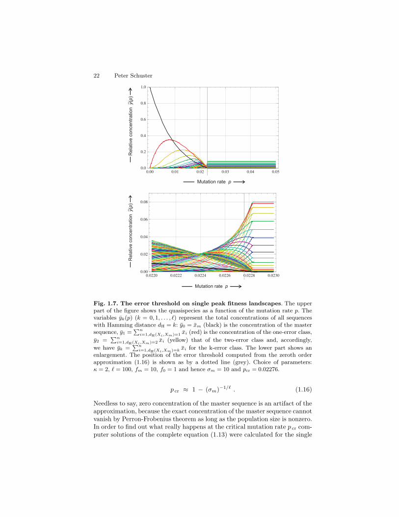
22 Peter Schuster

Fig. 1.7. The error threshold on single peak fitness landscapes. The upperpart of the figure shows the quasispecies as a function of the mutation rate p. Thevariables yk(p) (k = 0, 1, . . . , ℓ) represent the total concentrations of all sequenceswith Hamming distance dH = k: y0 = xm (black) is the concentration of the mastersequence, y1 =

∑n

i=1,dH(Xi,Xm)=1 xi (red) is the concentration of the one-error class,

y2 =∑n

i=1,dH(Xi,Xm)=2 xi (yellow) that of the two-error class and, accordingly,

we have yk =∑n

i=1,dH(Xi,Xm)=kxi for the k-error class. The lower part shows an

enlargement. The position of the error threshold computed from the zeroth orderapproximation (1.16) is shown as by a dotted line (grey). Choice of parameters:κ = 2, ℓ = 100, fm = 10, f0 = 1 and hence σm = 10 and pcr = 0.02276.

p cr ≈ 1 − (σm)−1/ℓ . (1.16)

Needless to say, zero concentration of the master sequence is an artifact of theapproximation, because the exact concentration of the master sequence cannotvanish by Perron-Frobenius theorem as long as the population size is nonzero.In order to find out what really happens at the critical mutation rate p cr com-puter solutions of the complete equation (1.13) were calculated for the single


peak fitness landscape.14 These calculations [75] show a sharp transition fromthe ordered quasispecies to the uniform distribution, xj = κ−ℓ ∀ j = 1, . . . , κℓ.At the critical mutation rate p cr replication errors accumulate and (indepen-dently of initial conditions) all sequences are present at the same frequency inthe long time limit as is reflected by the uniform distribution. The uniform dis-tribution is the exact solution of the eigenvalue problem at equal probabilitiesfor all nucleotide incorporations (A→A, A→U, A→G, and A→C) occurringat p = κ−1. The interesting aspect of the error threshold phenomenon consistsin the fact that the quasispecies approaches the uniform distribution at a thecritical mutation rate p cr, which is far below the random mutation value p.As a matter of fact the appearance of an error threshold and its shape dependon details of the fitness landscape [76, pp.51-60]. Some landscapes show noerror threshold at all but a smooth transition to the uniform distribution [77].More realistic fitness landscapes with a distribution of fitness values reveal amuch more complex situation: For constant superiority the value of p cr be-comes smaller with increasing variance of fitness values. The error thresholdphenomenon can be split into three different observations that coincide onthe single peak landscape: (i) vanishing of the master sequence xm, (ii) phasetransition like behavior, and (iii) transition to the uniform distribution. Onsuitable model landscapes the three observations do not coincide and thus canbe separated [78, 79].

How do populations behave at mutation rates above the error threshold?In reality a uniform distribution of variants as requested for the stationarystate can’t be realized. In RNA selection experiments population sizes hardlyexceed 1015 molecules, the smallest aptamers have chain lengths of ℓ = 27nucleotides [80] and this implies 427 ≈ 18 × 1015 different sequences. Even inthis most favorable case we are dealing with more sequences than moleculesin the population: a uniform distribution cannot exist. Although the origin ofthe lack of selective power is completely different – high mutation rates wipingout the differences in fitness values versus fitness differences being zero or toosmall for selection, the most likely scenarios to occur are migrating populationssimilar to evolution on a flat landscape [81]. Bernard Derrida and Luca Pelitifind that the populations break up into clones, which migrate into differentdirections in sequence space. Migrating populations are unable to conserve agenotype over generations, and unless a large degree of neutrality allows formaintenance of a phenotype despite changing genotypes, evolution becomesimpossible because inheritance breaks down.

Because of high selection pressure resulting from the hosts’ defense sys-tems virus population operate at mutations rates as high as possible in order

14 The single peak fitness landscape is a kind of mean field approximation: A fitnessvalue fm is assigned to the master sequence, whereas all other variants have thesame fitness f0. For this particular landscape the position x

(0)m = 0 calculated

within the zeroth-order approximation almost coincides with the position of thecritical change in the population structure (Fig.1.7).

24 Peter Schuster

to allow for fast evolution, and this is just below the error threshold [82]. In-creasing the mutation rate should drive the virus population beyond thresh-old where sufficiently accurate replication is no more possible. Therefore viruspopulations are doomed to die out at mutation rates above threshold andthis suggested a novel antiviral strategy that has led to the development ofnew drugs [83]. A more recent discussion of the error threshold phenomenontries to separate the error accumulation phenomenon from mutation causedfitness effects leading to virus extinction called lethal mutagenesis [84,85]. Asa matter of fact lethal mutagenesis describes the error threshold phenomenonfor variable population size N as required for limN → 0, but an analysisof population dynamics without and with stochastic effects at the onset ofmigration of populations is still missing. In addition, more detailed kineticstudies on replication in vitro near the error threshold are required before themechanism of virus extinction at high mutation rates will be understood.

Sequence-structure mappings of nucleic acid molecules (1.4) and proteinsprovide ample evidence for neutrality in the sense that many genotypes giverise to the same phenotype and identical or almost identical fitness valuesthat cannot be discriminated by natural selection. The possible occurrence ofneutral variants has been discussed already by Charles Darwin [2, chapter iv].Based on the results of the first sequence data from molecular biology MotooKimura formulated his neutral theory of evolution [86,87]. In absence of fitnessdifferences between variants random selection occurs because of stochastic en-hancement through autocatalytic processes: More frequent variants are morelikely to be replicated than less frequent ones. Ultimately a single genotypebecomes fixated in the population. The average time of replacement for adominant genotype is the reciprocal mutation rate, ν−1 = (ℓp)−1, which, in-terestingly, is independent of the population size. Are Kimura’s results validalso for large population sizes and high mutation rates as they occur, forexample, with viruses? Mathematical analysis [88] together with recent com-puter studies [78] yields the answer: Random selection in the sense of Kimuraoccurs only for sufficiently distant (master) sequences. In full agreement withthe exact result in the limit p→ 0 we find that two fittest sequences of Ham-ming distance dH = 1, two nearest neighbors in sequence space, are selectedas a strongly coupled pair with equal frequency of both members. Numeri-cal results demonstrate that this strong coupling occurs not only for smallmutation rates but extends over the whole range of p-values from p = 0 tothe error threshold p = pcr. For clusters of more than two Hamming distanceone sequences the frequencies of the individual members of the cluster is de-termined by the largest eigenvector of the adjacency matrix. Pairs of fittestsequences with Hamming distance dH = 2, i.e. two next nearest neighborswith two sequences in between, are also selected together but the ratio ofthe two frequencies is different from one. Again coupling extends from zeromutation rates to the error threshold. Strong coupling of fittest sequencesmanifests itself in virology as systematic deviations from consensus sequencesof populations as indeed observed in nature. For two fittest sequences with


dH ≥ 3 random selection chooses arbitrarily one of both and eliminates theother one as predicted by the neutral theory.

The function φ(t) was introduced as the mean fitness of a population inorder to allow for straightforward normalization of the population variables.A more general interpretation considers φ(t) as a flux out of the system. Thenthe equation describing evolution of the column vector of particle numbersN = (N1, . . . , Nn) is of the form [89]

dNj

dt= Fj(N) − Nj

C(t)φ(t) , i = 1, . . . , n ,

where Fj(N) is the function of unconstrained reproduction. An example isprovided by equation (1.13): Fj(N) =

∑ni=1QjifiNi. Explicit insertion of

the total concentration C(t) =∑n

i=1Ni(t) yields

φ(t) =

n∑

i=1

Fi(N) − dC

dtor C(t) = C0 +

∫ t

0

(

n∑

i=1

Fi(N) − φ(τ)

)

dτ .

Either C(t) or φ(t) can be chosen freely, the second function is then determinedby the equation given above. For normalized variables we find

dxj

dt=

1

C(t)

(

Fj(N) − xj

n∑

i=1

Fj(N)

)

.

For a large number of examples and for the most cases important in evolutionthe functions Fj(N) are homogeneous functions in N . For homogeneity ofdegree γ we have Fj(N) = Fj(C · N) = CγFj(x) and find

dxj

dt= Cγ−1

(

Fj(x) − xj

n∑

i=1

Fj(x)

)

, j = 1, . . . , n . (1.17)

Two conclusions can be drawn from this equation: (i) For γ = 1, e.g. theselection equation (1.4) or the replication-mutation equation (1.13), the de-pendence on the total concentration C vanishes and the solution curves innormalized variables xj(t) are the same in stationary (C = const) and non-stationary systems as long as C(t) remains finite and does not vanish, and (ii)if γ 6= 1 the long term behavior determined by x = 0 is identical for station-ary and non-stationary systems unless the population dies out C(t) → 0 orexplodes C(t) → ∞.

26 Peter Schuster

1.6 Evolution as a stochastic process

Stochastic phenomena are essential for evolution – each mutant after all startsout from a single copy and a large number of studies have been conductedon stochastic effects in population genetics [90]. Not too much work, however,has been devoted so far to the development of a general stochastic theoryof molecular evolution. We mention two examples representative for others[91, 92]. In the latter case the reaction network for replication and mutationwas analyzed as a multi-type branching process and it was proven that thestochastic process converges to the deterministic equation (1.13) in the limitof large populations. What is still missing is a comprehensive treatment, forexample by means of chemical master equations [93]. Then the deterministicpopulation variables xj(t) are replaced by stochastic variables Xj(t) and thecorresponding probabilities

P(j)k (t) = Prob{Xj = k} , k = 0, 1, . . . , N ; j = 1, . . . , n . (1.18)

The chemical master equation translates a mechanism into a set of differentialequation for the probabilities. The pendant of equation (1.13), for example,is the master equation

dP(j)k

dt=

(

n∑

i=1

Qjifi

n∑

s=1

s P (i)s

)

P(j)k−1 − φ(t)P

(j)k −

−(

n∑

i=1

Qjifi

n∑

s=1

s P (i)s

)

P(j)k + φ(t)P

(j)k+1 .

(1.19)

The only quantity that has to be specified further in this equation is theflux term φ(t). For the stochastic description it is not sufficient to have aterm that is just compensating the increase in population size due to replica-tion, a detailed model of the process is required. Examples are (i) the Moranprocess [94–96] with strictly constant population size and (ii) the flow reac-tor (CSTR) with a population size fluctuating within the limits of a

√N -

law [97, 98].15 The Moran process assumes that for every newborn moleculeone molecule is instantaneously eliminated. Strong coupling of otherwise com-pletely independent processes has the advantage of mathematical simplicitybut it is lacking a physical background. The flowreactor, on the other hand, isharder to treat in the mathematical analysis but it is based on solid physicalgrounds and can be easily implemented experimentally. In computer simula-tion both models require comparable efforts and for molecular systems pref-erence is given therefore to the flowreactor.

15 All thermodynamically admissible processes obey a so-called√

N law: For a meanpopulation size of N the actual population size fluctuates with a standard devi-ation proportional to

√N .


initial state

target

extinction

replication, mutation

and dilution

stock solution reaction mixture

a r0 * r•

10 12 14 16 18 20 22

population size N

0.2

0.0

0.4

0.6

0.8

1.0

pro

ba

bili

ty to

re

ach

ta

rge

t str

uctu

re

AUGC

GC

Fig. 1.8. Survival in the flowreactor. Replication and mutation in the flowreac-tor is implemented according to the mechanism (1.20). The stochastic process hastwo absorbing states: (i) extinction, Xj = 0∀ j = 1, . . . , n, and (ii) a predefinedtarget state – here the structure of tRNAphe. A rather sharp transition in the longtime behavior of the population is shown in the lower plot: Populations of naturalsequences (AUGC) switch from almost certain extinction to almost certain survivalin the range 13 ≤ N ≤ 18 and for binary sequences (GC) the transition is evensharper but requires slightly larger population sizes.

28 Peter Schuster

For evolution of RNA molecules through replication and mutation in theflowreactor, the following reaction mechanism has been implemented:

∗a0 r

−−−−→ A ,

A + Xi

Qjifi

−−−−→ Xi + Xj ; i, j = 1, . . . , n ,

Ar

−−−−→ ∅ , and

Xj

r

−−−−→ ∅ ; j = 1, . . . , n .

(1.20)

Stock solution is flowing into the reactor with a flow rate r and it feeds the re-actor with the material required for polynucleotide synthesis – schematicallydenoted by A and consisting, for example, of activated nucleotides, ATP,UTP, GTP and CTP as well as a replicating enzyme – into the system. Theconcentration of A in the stock solution is denoted by a0. The molecules Xj

are produced by the second reaction either by correct copying or by muta-tion. The third and the fourth reaction describe the outflux of material andcompensate the increase in volume caused by the influx of stock solution.The reactor is assumed to be perfectly mixed at every instant (continuousstirred-tank reactor = CSTR). For target search the stochastic process in thereactor is constructed to have two absorbing states (Fig.1.8): (i) extinction –all RNA molecules are diluted out of the reaction vessel, and (ii) survival – thepredefined target structure has been produced in the reactor. The populationsize determines the outcome of the computer experiment: Below populationsizes of N = 13 the reaction in the CSTR goes almost certainly extinct but itreaches the target with a probability close to one for N > 20. The probabilityof extinction is very small for sufficiently large populations and for populationsizes, N ≥ 1000, as reported here, extinction has been never observed.

In order to simulate the interplay between mutation acting on the RNAsequence and selection operating on RNA structures, the sequence-structuremap has to be turned into an integral part of the model [97, 98, 103]. Thesimulation tool starts from a population of RNA molecules and simulateschemical reactions corresponding to replication and mutation in a CSTR ac-cording to (1.20) by using Gillespie’s algorithm [99–101]. Molecules replicatein the reactor and produce both correct copies and mutants, the materialsto be consumed are supplied by the continuous influx of stock solution intothe reactor, and excess volume is removed by means of the outflux of reactorsolution. Two kinds of computer experiments were performed: Optimizationsof properties on a landscape derived from the sequence-structure map andtarget searches in shape space where the target is some predefined structure.

Early simulations optimizing replication rates in populations of binary GC-sequences yielded two general results:(i) The progress in evolution is stepwise rather than continuous as short adap-tive phases are interrupted by long quasistationary epochs [97, 98].


Fig. 1.9. A trajectory of evolutionary optimization. The topmost plot presents themean distance to the target structure of a population of 1000 molecules. The plotin the middle shows the width of the population in Hamming distance between se-quences and the plot at the bottom is a measure of the velocity with which the centerof the population migrates through sequence space. Diffusion on neutral networkscauses spreading on the population in the sense of neutral evolution [102]). A re-markable synchronization is observed: At the end of each quasistationary plateau anew adaptive phase in the approach towards the target is initiated, which is accom-panied by a drastic reduction in the population width and a jump in the populationcenter (The top of the peak at the end of the second long plateau is marked bya black arrow). A mutation rate of p = 0.001 was chosen, the replication rate pa-rameter is defined in equation (1.21), and initial and target structures are shown intable 1.1.

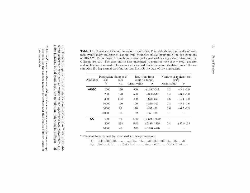
30

Peter

Sch

uster

Table 1.1. Statistics of the optimization trajectories. The table shows the results of sam-pled evolutionary trajectories leading from a random initial structure SI to the structureof tRNAphe, ST as target. a Simulations were performed with an algorithm introduced byGillespie [99–101]. The time unit is here undefined. A mutation rate of p = 0.001 per siteand replication was used. The mean and standard deviation were calculated under the as-sumption if a log-normal distribution that fits well the data of the simulations.

Population Number of Real time from Number of replicationsAlphabet size runs start to target [107]

N nR Mean value σ Mean value σ

AUGC 1000 120 900 +1380 -542 1.2 +3.1 -0.9

2000 120 530 +880 -330 1.4 +3.6 -1.0

3000 1199 400 +670 -250 1.6 +4.4 -1.2

10000 120 190 +230 -100 2.3 +5.3 -1.6

30000 63 110 +97 -52 3.6 +6.7 -2.3

100000 18 62 +50 -28 – –

GC 1000 46 5160 +15700 -3890 – –

3000 278 1910 +5180 -1460 7.4 +35.8 -6.1

10000 40 560 +1620 -420 – –

a The structures SI and ST were used in the optimization:

SI : ((.(((((((((((((............(((....)))......)))))).))))))).))...(((......)))

ST : ((((((...((((........)))).(((((.......))))).....(((((.......))))).))))))....

(ii)D

ifferen

tco

mputer

runs

with

iden

ticalin

itialco

nditio

ns16

resulted

indif-

ferent

structu

resw

ithsim

ilar

valu

esfo

rth

eoptim

izedra

tepara

meters.

De-

spite

iden

tical

initia

lco

nditio

ns,

the

popula

tions

mig

rated

indiff

erent

–al-

16

Identica

lm

eans

here

that

every

thin

gin

the

com

puter

runs

was

the

sam

eex

cept

the

seeds

for

the

random

num

ber

gen

erato

rsand

this

implies

diff

erent

seriesof

random

even

ts.


most orthogonal – directions in sequence space and gave rise to contingencyin evolution thereby [98].

In target search problems the replication rate of a sequence Xk, repre-senting its fitness fk, is chosen to be a function of the Hamming distance17

between the structure formed by the sequence, Sk = f(Xk) and the targetstructure ST ,

fk(Sk, ST ) =1

α + dH(Sk, ST )/ℓ, (1.21)

which increases when Sk approaches the target (α is an empirically adjustableparameter that was commonly chosen to be 0.1). A trajectory is completedwhen the population reaches a sequence that folds into the target structure –appearance of the target structure in the population is defined as an absorb-ing state of the stochastic process. A typical trajectory is shown in fig.1.9. Inthis simulation a homogenous population consisting on N molecules with thesame random sequence and structure is chosen as initial condition. The tar-get structure is the well-known secondary structure of phenylalanyl-transferRNA (tRNAphe). The mean distance to target of the population decreases insteps until the target is reached [103–105] and, again the approach to targetis stepwise rather than continuous: Short adaptive phases are interrupted bylong quasistationary epochs. In order to reconstruct optimization dynamics,a time ordered series of structures was determined that leads from an initialstructure SI to the target structure ST . This series, called relay series, is auniquely defined and uninterrupted sequence of shapes. It is retrieved throughbacktracking, that is in opposite direction from the final structure to the ini-tial shape. The procedure starts by highlighting the final structure and tracesit back during its uninterrupted presence in the flow reactor until the time ofits first appearance. At this point we search for the parent shape from whichit descended by mutation. Now we record time and structure, highlight theparent shape, and repeat the procedure. Recording further backwards yieldsa series of shapes and times of first appearance which ultimately ends in theinitial population.18 Usage of the relay series and its theoretical backgroundallows for classification of transitions [103, 104, 106]. Inspection of the relayseries together with the sequence record on the quasistationary plateaus pro-vides strong hints for the distinction of two scenarios:(i) The structure is constant and we observe neutral evolution in the sense ofKimura’s theory of neutral evolution [87]. In particular, the numbers of neu-tral mutations accumulated are proportional to the number of replications inthe population, and the evolution of the population can be understood as a

17 The distance between two structures is defined here as the Hamming distancebetween the two symbolic notations of the structures.

18 It is important to stress two facts about relay series: (i) The same shape may ap-pear two or more times in a given relay series series. Then, it was extinct betweentwo consecutive appearances. (ii) A relay series is not a genealogy which is thefull recording of parent-offspring relations in a time-ordered series of genotypes.

32 Peter Schuster

diffusion process on the corresponding neutral network [102].(ii) The process during the quasistationary epoch involves several closely re-lated structures with identical replication rates and the relay series reveals akind of random walk in the space of these neutral structures.The diffusion of the population on the neutral network is illustrated by theplot in the middle of fig.1.9 that shows the width of the population as a func-tion of time [105]. The population width increases during the quasistationaryepoch and sharpens almost instantaneously after a sequence had been createdby mutation that allows for the start of a new adaptive phase in the optimiza-tion process. The scenario at the end of the plateau corresponds to a bottleneck of evolution. The lower part of the figure shows a plot of the migrationrate or drift of the population center and confirms this interpretation: Mi-gration of the population center is almost always very slow unless the center‘jumps’ from one point in sequence space to a possibly distant point wherethe molecule initiating the new adaptive phase is located. A closer look atthe three curves in fig.1.9 reveals coincidence of three events: (i) collapse-likenarrowing of the population spread, (ii) jump-like migration of the populationcenter, and (iii) beginning of a new adaptive phase.

It is worth mentioning that the optimization behavior observed in a long-term evolution experiment with Escherichia coli [46] can be readily inter-preted in terms of random searches on a neutral network. Starting with twelvecolonies in 1988, Lenski and his coworkers observed after 31 500 generation ortwenty years a great adaptive innovation in one colony [45]: This colony de-veloped a kind of membrane channel that allows for uptake of citrate, which isused as buffer in the medium. The colony thus conquered a new resource thatled to a substantial increase in colonial growth. The mutation providing cit-rate import into the cell is reproducible when earlier isolates of this particularcolony are used for a restart of the evolutionary process. Apparently this par-ticular colony has traveled through sequence space to a position from wherethe adaptive mutation allowing for citrate uptake is within reach. All othereleven colonies did not give rise to mutations with a similar function. Theexperiment is a nice demonstration of contingency in evolution: The conquestof the citrate resource does not happen through a single highly improbablemutation but by means of a mutation with standard probability from a par-ticular region of sequence space where the population had traveled in one caseout of twelve – history matters, or repeating Theodosius Dobzhansky’s famousquote: “Nothing makes sense in biology except in the light of evolution” [29].

Table 1.1 collects some numerical data sampled from evolutionary trajecto-ries of simulations repeated under identical conditions. Individual trajectoriesshow enormous scatter in the time or the number of replications required toreach the target. The mean values and the standard deviations were obtainedfrom statistics of trajectories under the assumption of log-normal distribu-tions. Despite the scatter three features are unambiguously detectable:(i) The search in GC sequence space takes about five time as long as the cor-responding process in AUGC sequence space in agreement with the difference


in neutral network structure.(ii) The time to target decreases with increasing population size.(iii) The number of replications required to reach target increases with pop-ulation size.Combination of the results (ii) and (iii) allows for a clear conclusion concerningtime and material requirements of the optimization process: Fast optimizationrequires large populations whereas economic use of material suggests to workwith small population sizes just sufficient to avoid extinction.

A study of parameter dependence of RNA evolution was reported in arecent simulation [107]. Increase in mutation rate leads to an error thresholdphenomenon that is closely related to one observed with quasispecies on asingle-peak landscape as described above [69, 75]. Evolutionary optimizationbecomes more efficient19 with increasing error rate until the error thresholdis reached. Further increase in error rates leads to a breakdown of the opti-mization process. As expected the distribution of replication rates or fitnessvalues fk in sequence space is highly relevant too: Steep decrease of fitnesswith the distance to the master structure represented by the target, whichhas the highest fitness value, leads to sharp threshold behavior as observedon single-peak landscapes, whereas flat landscapes show a broad maximum ofoptimization efficiency without an indication of threshold-like behavior.

1.7 Concluding remarks

Biology developed differently from physics because it refrained from usingmathematics as a tool to analyze and unfold theoretical concepts. Applica-tion of mathematics enforces clear definitions and reduction of observationsto problems that can be managed. Over the years physics became the sci-ence of abstractions and generalizations, biology the science of encyclopediasof special cases with all their beauties and peculiarities. Among others thereis one exception of the rule: Charles Darwin presented a grand generaliza-tion derived from a wealth of personal and reported observations togetherwith knowledge from economics concerning population dynamics. In the sec-ond half of the twentieth century the appearance of molecular biology onthe stage changed the situation entirely. A bridge was built from physics andchemistry to biology and mathematical models from biochemical kinetics orpopulation genetics became presentable in biology. Nevertheless, the vast ma-jority of biologists still smiled at the works of theorists. Molecular genetics bythe end of the twentieth century created such a wealth of data that almosteverybody feels nowadays that progress cannot be made without a compre-hensive theoretical foundation and a rich box of suitable computational tools.Nothing like this is at hand but indications for attempts in the right direction

19 Efficiency of evolutionary optimization is measured by average and best fitnessvalues obtained in populations after a predefined number of generations.

34 Peter Schuster

are already visible. Biology is going to enter the grand union of science thatstarted with physics and chemistry and is progressing fast. Molecular biologystarted out with biomolecules in isolation and deals now with cells, organs,and organisms. Hopefully, this spectacular success will end the so far fruitlessreductionism versus holism debate.

Insight into the mechanisms of evolution reduced to the conceivablymost simple systems was provided here. These systems deal with evolvablemolecules in cell-free assays and are accessible by rigorous mathematical anal-ysis and physical experimentation. An extension to asexual species, in partic-ular viruses and bacteria, is within reach. The molecular approach providesa simple explanation why we have species for this organisms despite the factthat there is neither restricted recombination nor reproductive isolation. Thesequence spaces are so large that populations, colonies or clones can migratefor the age of the universe without coming close to another asexual species.We can give an answer to the question of the origin of complexity: Complexityin evolution results primarily from genotype-phenotype relations and from theinfluences of the environment. Evolutionary dynamics may be complicated insome cases but it is not complex at all. This has been reflected already by thesequence-structure map of our toy example. Conformation spaces dependingon the internal folding kinetics as well as on environmental conditions andcompatible sets are metaphors for more complex features in evolution proper.

Stochasticity is still an unsolved problem in molecular evolution. Themathematics of stochastic processes encounters difficulties in handling theequations of evolution in detail. A comprehensive stochastic theory is still notat hand and the simulations are lacking more systematic approaches sincecomputer simulations of chemical kinetics of evolution are in an early statetoo. Another fundamental problem concerns the spatial dimensions: Almostall treatments are assuming spatial homogeneity but we have evidence for thesolid particle like structure of the chemical factories of the cell. In the future,any comprehensive theory of the cell will have to deal with these structurallyrich supramolecular structures too.

References

1. G. Galilei, Il Saggiatore, vol. 6, p.232 (Edition Nationale, Florence, IT, 1896).English Translation from Italian Original

2. C. Darwin, On the Origin of Species by Means of Natural Selection or the

Preservation of Favoured Races in the Struggle for Life (John Murray, London,1859)

3. E. Mayr, The Growth of Biological Thought. Diversity, Evolution, and Inher-

tiance (The Belknap Press of Harvard University Press, 1982)4. G. Mendel, Verhandlungen des naturforschenden Vereins in Brunn 4, 3 (1866)5. G. Mendel, Verhandlungen des naturforschenden Vereins in Brunn 8, 26 (1870)6. G.A. Nogler, Genetics 172, 1 (2006)


7. T.R. Malthus, An Essay of the Principle of Population as it Affects the Future

Improvement of Society (J. Johnson, London, 1798)8. R.A. Fisher, The Genetical Theory of Natural Selection (Oxford University

Press, Oxford, UK, 1930)9. J.B.S. Haldane, The Causes of Evolution (Longmans Green, London, 1932).

Reprinted 1990 in the Princeton Science Library by Princeton University Press,Princeton, NJ

10. S. Wright, Evolution and the Genetics of Populations, vol. 1-4 (University ofChicago Press, Chicago, IL, 1968, 1969, 1977, 1978)

11. A.J. Lotka, Elements of Physical Biology (Williams & Wilkins, Baltimore, MD,1925)

12. V. Volterra, Mem.R.Accad.Naz. dei Lincei Ser.VI/2, 31 (1926)13. E.P. Odum, Fundamentals of Ecology (W. B. Saunders Company, Philadelphia,

PA, 1953)14. R.M. May (ed.), Theoretical Ecology. Principles and Applications (Blackwell

Scientific Publications, Oxford, UK, 1976)15. A.M. Turing, Phil. Trans. Roy. Soc. London Ser. B 237, 37 (1952)16. A.G. und Hans Meinhardt, Kybernetik 12, 30 (1972)17. H. Meinhardt, Models of Biological Pattern Formation (Academic Press, Lon-

don, 1982)18. J.D. Murray, Scientific American 258(3), 62 (1988)19. J.D. Murray, Mathematical Biology II: Spatial Models and Biomedical Appli-

cations, 3rd edn. (Springer-Verlag, New York, 2003)20. A.L. Hodgkin, A.F. Huxley, J. Physiology 117, 500 (1952)21. J.J. Hopfield, Proc. Natl. Acad. Sci. USA 79, 2554 (1982)22. H. Judson, The Eighth Day of Creation. The Makers of the Revolution in Bi-

ology (Jonathan Cape, London, 1979)23. A. Maxam, W. Gilbert, Proc. Natl. Acad. Sci. USA 74, 560 (1977)24. F. Sanger, S. Nicklen, A. Coulson, Proc. Natl. Acad. Sci. USA 74, 5463 (1977)25. J. Dale, M. von Schantz, Form Genes to Genomes: Concepts and Applications

of DNA Technology (Wiley-VCh, New York, 2007)26. S. Brenner, The Scientist 16(4), 14 (2002)27. J.S. Edwards, M. Covert, B.O. Palsson, Environ.Microbiol. 4, 133 (2002)28. H.W. Engl, C. Flamm, P. Kugler, J. Lu, S. Muller, P. Schuster, Inverse Prob-

lems 25, 123014 (2009)29. T. Dobzhansky, F.J. Ayala, G.L. Stebbins, J.W. Valentine, Evolution (W. H.

Freeman & Co., San Francisco, CA, 1977)30. L. Euler, Introductio in Analysin Infinitorum, 1748. English Translation: John

Blanton, Introduction to Analysis of the Infinite, vol. I and II (Springer-Verlag,Berlin, 1988)

31. P. Verhulst, Corresp. Math. Phys. 10, 113 (1838)32. D. Zwillinger, Handbook of Differential Equations, 3rd edn. (Academic Press,

San Diego, CA, 1998)33. M. Eigen, Naturwissenschaften 58, 465 (1971)34. J. Maynard-Smith, Nature 225, 563 (1970)35. R.W. Hamming, Coding and Information Theory, 2nd edn. (Prentice-Hall, En-

glewood Cliffs, NJ, 1986)36. J. Rogers, G. Joyce, Nature 402, 323 (1999)37. J.S. Reader, G.F. Joyce, Nature 420, 841 (2002)

36 Peter Schuster

38. P. Schuster, Physica D 107, 351 (1997)39. P. Gitchoff, G.P. Wagner, Complexity 2(1), 37 (1998)40. P.F. Stadler, R. Seitz, G.P. Wagner, Bull. Math. Biol. 62, 399 (2000)41. B.R.M. Stadler, P.F. Stadler, M. Shpak, G.P. Wagner, Z. Phys.Chem. 216,

217 (2002)42. D.E. Goldberg, Genetic Algorithms in Search, Optimization, and Machine

Learning (Addison-Wesley, Reading, MA, 1989)43. L.M. Schmitt, Theoret. Computer Science 259, 1 (2001)44. J.E. Barrick, D.S. Yu, H. Jeong, T.K. Oh, D. Schneider, R.E. Lenski, J.F. Kim,

Nature 441, 1243 (2009)45. Z.D. Blount, C. Z., R.E. Lenski, Proc. Natl. Acad. Sci. USA 105, 7898 (2008)46. R.E. Lenski, M.R. Rose, S.C. Simpson, S.C. Tadler, The American Naturalist

38, 1315 (1991)47. P. Schuster, Reports on Progress in Physics 69, 1419 (2006)48. M. Zuker, P. Stiegler, Nucleic Acids Research 9, 133 (1981)49. I.L. Hofacker, W. Fontana, P.F. Stadler, L.S. Bonhoeffer, M. Tacker, P. Schus-

ter, Mh.Chemie 125, 167 (1994)50. M. Zuker, Science 244, 48 (1989)51. S. Wuchty, W. Fontana, I.L. Hofacker, P. Schuster, Biopolymers 49, 145 (1999)52. C. Flamm, W. Fontana, I.L. Hofacker, P. Schuster, RNA 6, 325 (1999)53. M.T. Wolfinger, W.A. Svrcek-Seiler, C. Flamm, I.L. Hofacker, P.F. Stadler,

J. Phys.A: Math.Gen. 37, 4731 (2004)54. D.R. Mills, R.L. Peterson, S. Spiegelman, Proc. Natl. Acad. Sci. USA 58, 217

(1967)55. S. Spiegelman, Quart. Rev.Biophys. 4, 213 (1971)56. G.F. Joyce, Angew. Chem. Internat. Ed. 46, 6420 (2007)57. C.K. Biebricher, M. Eigen, J. William C. Gardiner, Biochemistry 22, 2544

(1983)58. C.K. Biebricher, M. Eigen, J. William C. Gardiner, Biochemistry 23, 3186

(1984)59. C.K. Biebricher, M. Eigen, J. William C. Gardiner, Biochemistry 24, 6550

(1985)60. S. Klussmann (ed.), The Aptamer Handbook. Functional Oligonucleotides and

Their Applications (Wiley-VCh Verlag, Weinheim, DE, 2006)61. A. Lescoute, N.B. Leontis, C. Massire, E. Westhof, Nucleic Acids Res. 33, 2395

(2005)62. N.B. Leontis, A. Lescoute, E. Westhof, Curr.Opinion Struct.Biol. 16, 279

(2006)63. I.L. Hofacker, P. Schuster, P.F. Stadler, Discr. Appl.Math. 89, 177 (1998)64. J.S. McCaskill, Biopolymers 29, 1105 (1990)65. M. Mandal, B. Boese, J.E. Barrick, W.C. Winkler, R.R. Breaker, Cell 113,

577 (2003)66. C.J. Thompson, J.L. McBride, Math. Biosci. 21, 127 (1974)67. B.L. Jones, R.H. Enns, S.S. Rangnekar, Bull. Math.Biol. 38, 15 (1976)68. M. Eigen, P. Schuster, Naturwissenschaften 64, 541 (1977)69. M. Eigen, J. McCaskill, P. Schuster, Adv.Chem. Phys. 75, 149 (1989)70. E. Seneta, Non-negative Matrices and Markov Chains, 2nd edn. (Springer-

Verlag, New York, 1981)71. N. Rohde, H. Daum, C.K. Biebricher, J. Mol. Biol. 249, 754 (1995)


72. E. Domingo, D. Szabo, T. Taniguchi, C. Weissmann, Cell 13, 735 (1978)73. E. Domingo, J. Holland, in RNA Genetics. Vol.III: Variability of Virus

Genomes, vol. III, ed. by E. Domingo, J. Holland, P. Ahlquist (CRC Press,Boca Raton, FL, 1988), pp. 3–36

74. E. Domingo (ed.), Quasispecies: Concepts and Implications for Virology

(Springer-Verlag, Berlin, 2006)75. J. Swetina, P. Schuster, Biophys. Chem. 16, 329 (1982)76. P.E. Phillipson, P. Schuster, Modeling by Nonlinear Differential Equations. Dis-

sipative and Conservative Processes, World Scientific Series on Nonlinear Sci-

ence A, vol. 69 (World Scientific, Singapore, 2009)77. T. Wiehe, Genet. Res. Camb. 69, 127 (1997)78. P. Schuster, Theory in Biosciences 129 (2010). Submitted79. P. Schuster. Quasispecies and error thresholds on realistic fitness landscapes

(2010). Preprint80. L. Jiang, A.K. Suri, R. Fiala, D.J. Patel, Chemistry &Biology 4, 35 (1997)81. B. Derrida, L. Peliti, Bull. Math. Biol. 53, 355 (1991)82. J.W. Drake, Proc. Natl. Acad. Sci. USA 90, 4171 (1993)83. E. Domingo, ed., Virus Research 107(2), 115 (2005)84. J.J. Bull, L. Ancel Myers, M. Lachmann, PLoS Comp. Biol. 1, 450 (2005)85. J.J. Bull, R. Sanjuan, C.O. Wilke, J.Virology 81, 2930 (2007)86. M. Kimura, Nature 217, 624 (1968)87. M. Kimura, The Neutral Theory of Molecular Evolution (Cambridge University

Press, Cambridge, UK, 1983)88. P. Schuster, J. Swetina, Bull.Math. Biol. 50, 635 (1988)89. M. Eigen, P. Schuster, Naturwissenschaften 65, 7 (1978)90. R.A. Blythe, A. McKane, J. Stat.Mech.: Theor. Exp. p. P07018 (2007). DOI

10.1088/1742-5468/2007/07/P0701891. B.L. Jones, H.K. Leung, Bull. Math.Biol. 43, 665 (1981)92. L. Demetrius, P. Schuster, K. Sigmund, Bull. Math.Biol. 47, 239 (1985)93. C.W. Gardiner, Stochastic Methods. A Handbook for the Natural and Social

Sciences, 4th edn. Springer Series in Synergetics (Springer-Verlag, Berlin, 2009)94. P. Moran, Proc. Cambridge Philos. Soc. 54, 60 (1958)95. P. Moran, The Statistical Processes of Evolutionary Theory (Clarendon Press,

Oxford, UK, 1962)96. M.A. Nowak, Evolutionary Dynamics: Exploring the Equations of Life (The

Belknap Press of Harvard University Press, Cambridge, MA, 2006)97. W. Fontana, P. Schuster, Biophys. Chem. 26, 123 (1987)98. W. Fontana, W. Schnabl, P. Schuster, Phys.Rev.A 40, 3301 (1989)99. D.T. Gillespie, J. Comp.Phys. 22, 403 (1976)

100. D.T. Gillespie, J. Phys.Chem. 81, 2340 (1977)101. D.T. Gillespie, Annu.Rev.Phys. Chem. 58, 35 (2007)102. M.A. Huynen, P.F. Stadler, W. Fontana, Proc. Natl. Acad. Sci. USA 93, 397

(1996)103. W. Fontana, P. Schuster, Science 280, 1451 (1998)104. W. Fontana, P. Schuster, J.Theor.Biol. 194, 491 (1998)105. P. Schuster, in Evolutionary Dynamics – Exploring the Interplay of Accident,

Selection, Neutrality, and Function, ed. by J.P. Crutchfield, P. Schuster (OxfordUniversity Press, New York, 2003), pp. 163–215

106. B.R.M. Stadler, P.F. Stadler, G.P. Wagner, W. Fontana, J. Theor. Biol. 213,241 (2001)

107. A. Kupczok, P. Dittrich, J. Theor. Biol. 238, 726 (2006)

Index

adaptation, 2, 32

biologymolecular, 4

Brenner, Sydney, 4

complex systems, 2contingency, 31, 32

DarwinCharles, 2, 3, 5, 7, 8, 24, 33evolution, see optimization principleoptimization principle, 2, 8, 14Origin of Species, 2, 3

distanceHamming, 10, 12, 13, 24structure, 17

DNA sequencing, 4Dobzhansky, Theodosius, 5, 32

ecology, theoretical, 4Eigen, Manfred, 10, 20, 25, 33emergence, ontological, 2equation

mutation-selection, 19selection, 8Verhulst, 7

error class, see mutant classEuler, Leonhard, 7evolution

adaptive, see adaptationneutral, 24, 29

Fibonacci, 5

Liber abaci, 5Fisher, Ronald, 3fitness value, 7flow rate, 28flowreactor, 27, 28

Galilei, Galileo, 2growth, exponential, 3, 7

Haldane, J.B.S., 3Hodgkin

-Huxley model, 4Alan, 4

holism, 2Hopfield, John, 4Huxley, Andrew, 4hypercube, 10

Kimura, Motoo, 24, 31

landscapefitness, 23flat, 23, 28, 33free energy, 17, 19single peak, 22, 23, 33

Lenski, Richard, 13, 32lethal mutagenesis, 24Lotka-Volterra model, 4

Malthus, Robert, 3, 7mapping

genotype-phenotype, 13sequence-structure, 14, 16, 24, 28

Mayr, Ernst, 2, 3Mendel, Gregor, 3

40 Index

metric, 10, 13, 17multiplication, 2mutant class, 9, 10mutation, 10, 12, 13, 19, 20, 23, 26–28,

31, 32adaptive, 32neutral, 31point, 12, 13

mutation rate, 19–24, 29, 30, 33

networksneural, 4neutral, 16, 29, 32, 33

Perron-Frobenius theorem, 20, 22phase

adaptive, 28, 29, 31, 32quasistationary, 31, 32

population support, 12

quasispecies, 20, 22, 23, 33

recombination, 7, 12, 13, 34reductionists’ program, 2replication, 14, 19–21, 24, 26–28, 30–33replication error, see mutationreplication rate, 14, 19, 20, 28, 29, 31,

32reproduction, 2, 7, 10, 12, 14RNA switch, 19

selection, 3, 8, 9, 14, 23, 28

constraint, 7, 8natural, 2, 3, 5, 24pressure, 23random, 24, 25

sequenceconsensus, 11, 12

spacebinary sequence, 9, 10conformation, 17genotype, see sequence spacemetric, 10phenotype, see shape spacerecombination, 12sequence, 10, 12, 13, 16, 29, 31, 32shape, 13, 16

structureRNA secondary, 14

thresholderror, 21, 23, 24, 33mutation, see error threshold

transformintergrating factors, 8

TuringAlan, 4model, 4

variation, 2, 3Verhulst, Pierre-Francois, 7

Wright, Sewall, 3

1 physical principles of evolution

Documents