1

Peter Fox

Data Analytics – ITWS-4963/ITWS-6965

Week 7a, March 10, 2015

Labs: more data, models, prediction, deciding with trees

Assignment 6 on Website• Your term projects should fall within the scope of a data analytics

problem of the type you have worked with in class/ labs, or know of yourself – the bigger the data the better. This means that the work must go beyond just making lots of figures. You should develop the project to indicate you are thinking of and exploring the relationships and distributions within your data. Start with a hypothesis, think of a way to model and use the hypothesis, find or collect the necessary data, and do both preliminary analysis, detailed modeling and summary (interpretation). Grad students must develop two types of models.– Note: You do not have to come up with a positive result, i.e. disproving the hypothesis

is just as good.

• Introduction (2%)• Data Description (3%)• Analysis (5%)• Model Development (12%)• Conclusions and Discussion (3%)• Oral presentation (5%) (~5 mins)

2

Titanic – Bayes (from last week)

> data(Titanic)

> mdl <- naiveBayes(Survived ~ ., data = Titanic)

> mdl

3

Naive Bayes Classifier for Discrete PredictorsCall: naiveBayes.formula(formula = Survived ~ ., data = Titanic)A-priori probabilities:Survived No Yes 0.676965 0.323035 Conditional probabilities: ClassSurvived 1st 2nd 3rd Crew No 0.08187919 0.11208054 0.35436242 0.45167785 Yes 0.28551336 0.16596343 0.25035162 0.29817159 SexSurvived Male Female No 0.91543624 0.08456376 Yes 0.51617440 0.48382560 AgeSurvived Child Adult No 0.03489933 0.96510067 Yes 0.08016878 0.91983122 Try Lab6b_9_2014.R

Classification Bayes (last week)

• Retrieve the abalone.csv dataset• Predicting the age of abalone from physical

measurements. • Perform naivebayes classification to get

predictors for Age (Rings). Interpret.• Compare to what you got from kknn (weighted

nearest neighbors) in class 4b

4

http://www.ugrad.stat.ubc.ca/R/library/mlbench/html/HouseVotes84.

html > require(mlbench)

> data(HouseVotes84)

> model <- naiveBayes(Class ~ ., data = HouseVotes84)

> predict(model, HouseVotes84[1:10,-1])

[1] republican republican republican democrat democrat democrat republican republican republican

[10] democrat

Levels: democrat republican 5

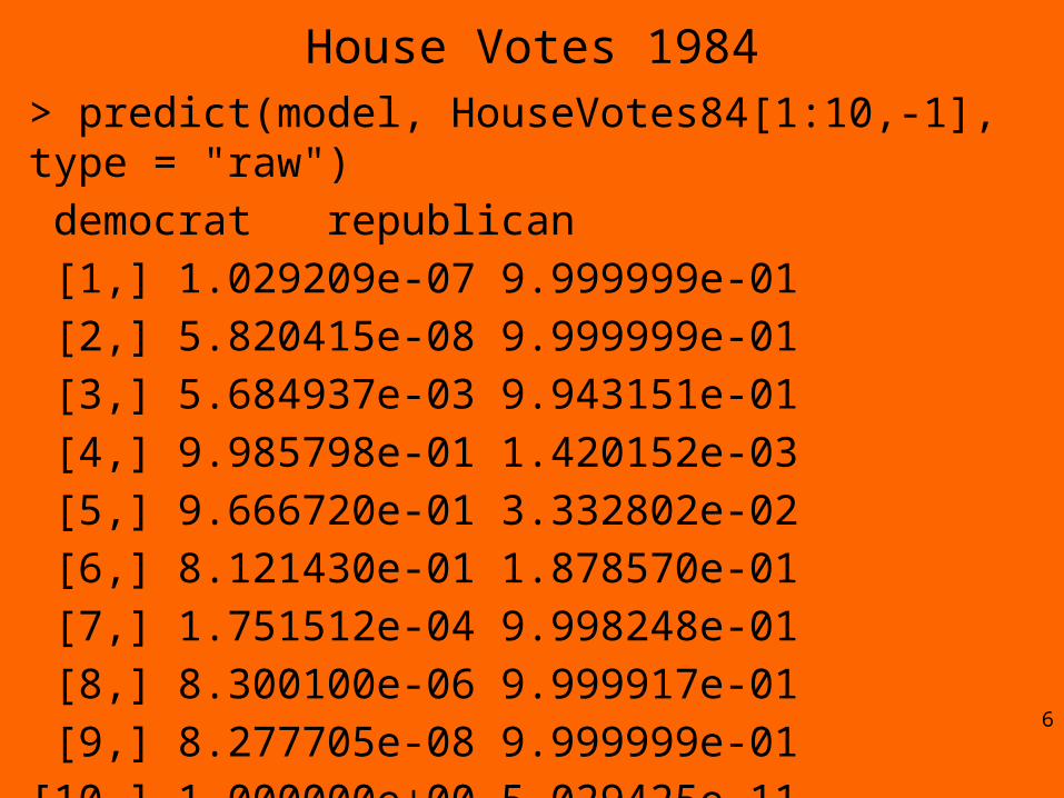
House Votes 1984> predict(model, HouseVotes84[1:10,-1], type = "raw")

democrat republican

[1,] 1.029209e-07 9.999999e-01

[2,] 5.820415e-08 9.999999e-01

[3,] 5.684937e-03 9.943151e-01

[4,] 9.985798e-01 1.420152e-03

[5,] 9.666720e-01 3.332802e-02

[6,] 8.121430e-01 1.878570e-01

[7,] 1.751512e-04 9.998248e-01

[8,] 8.300100e-06 9.999917e-01

[9,] 8.277705e-08 9.999999e-01

[10,] 1.000000e+00 5.029425e-116

House Votes 1984

> pred <- predict(model, HouseVotes84[,-1])

> table(pred, HouseVotes84$Class)

pred democrat republican

democrat 238 13

republican 29 155

7

Hair, eye color> data(HairEyeColor)

> mosaicplot(HairEyeColor)

> margin.table(HairEyeColor,3)

Sex

Male Female

279 313

> margin.table(HairEyeColor,c(1,3))

Sex

Hair Male Female

Black 56 52

Brown 143 143

Red 34 37

Blond 46 81

Construct a naïve Bayes classifier and test it! 8

Another example> A = c(1, 2.5); B = c(5, 10); C = c(23, 34)

> D = c(45, 47); E = c(4, 17); F = c(18, 4)

> df <- data.frame(rbind(A,B,C,D,E,F))

> colnames(df) <- c("x","y")

> hc <- hclust(dist(df))

> plot(hc)

> df$cluster <- cutree(hc,k=2) # 2 clusters

> plot(y~x,df,col=cluster)9

See also• Lab5a_ctree_1_2015.R

– Try clustergram instead– Try hclust

• Lab3b_kmeans1_2015.R– Try clustergram instead– Try hclust

10

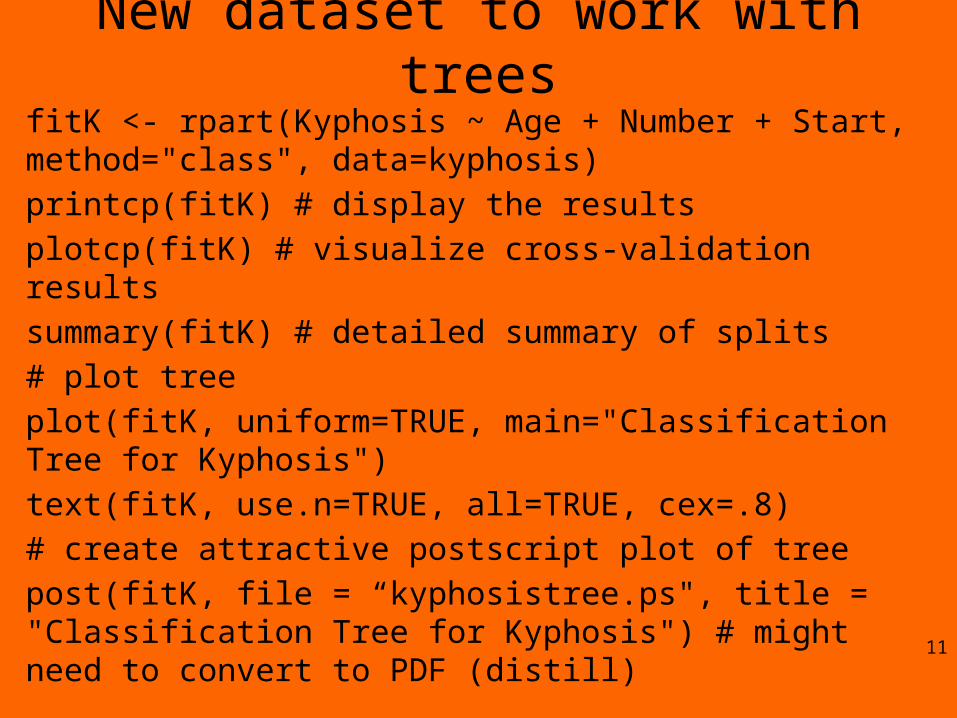
New dataset to work with treesfitK <- rpart(Kyphosis ~ Age + Number + Start, method="class", data=kyphosis)

printcp(fitK) # display the results

plotcp(fitK) # visualize cross-validation results

summary(fitK) # detailed summary of splits

# plot tree

plot(fitK, uniform=TRUE, main="Classification Tree for Kyphosis")

text(fitK, use.n=TRUE, all=TRUE, cex=.8)

# create attractive postscript plot of tree

post(fitK, file = “kyphosistree.ps", title = "Classification Tree for Kyphosis") # might need to convert to PDF (distill)

11

12

13

> pfitK<- prune(fitK, cp= fitK$cptable[which.min(fitK$cptable[,"xerror"]),"CP"])> plot(pfitK, uniform=TRUE, main="Pruned Classification Tree for Kyphosis")> text(pfitK, use.n=TRUE, all=TRUE, cex=.8)> post(pfitK, file = “ptree.ps", title = "Pruned Classification Tree for Kyphosis”)

14

> fitK <- ctree(Kyphosis ~ Age + Number + Start, data=kyphosis)> plot(fitK, main="Conditional Inference Tree for Kyphosis”)

15

> plot(fitK, main="Conditional Inference Tree for Kyphosis",type="simple")

Swiss - scatterplotMatrix

16

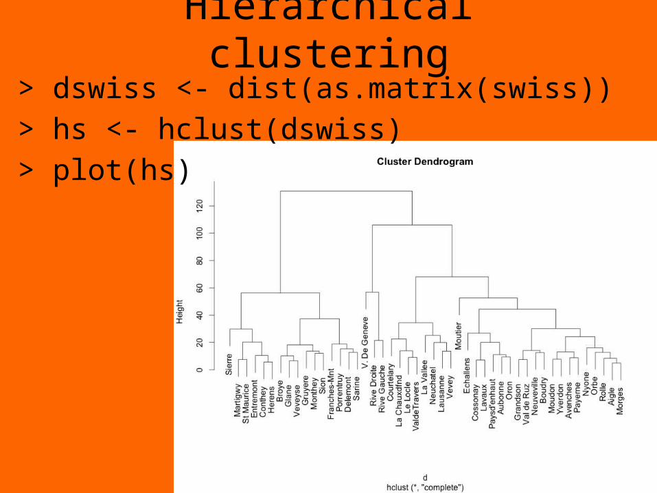
Hierarchical clustering

17

> dswiss <- dist(as.matrix(swiss))

> hs <- hclust(dswiss)

> plot(hs)

ctree

18

require(party)

swiss_ctree <- ctree(Fertility ~ Agriculture + Education + Catholic, data = swiss)

plot(swiss_ctree)

19

How could you get this?

Rpart – recursive partitioning

20

require(rpart)

Swiss_rpart <- rpart(Fertility ~ Agriculture + Education + Catholic, data = swiss)

plot(swiss_rpart) # try some different plot options

text(swiss_rpart) # try some different text options

# try other data

Rpart – recursive partitioning

21

Try this for “Rings” on the Abalone dataset

Try ctree – compare – we’ll discuss these Friday

But if you do the ctree you may want to “try pruning”

Mileage dataset.# Regression Tree Example

require(rpart)

# build the tree

fitM <- rpart(Mileage~Price + Country + Reliability + Type, method="anova", data=cu.summary)

printcp(fitM) # display the results….

Root node error: 1354.6/60 = 22.576

n=60 (57 observations deleted due to missingness)

CP nsplit rel error xerror xstd

1 0.622885 0 1.00000 1.03165 0.176920

2 0.132061 1 0.37711 0.51693 0.102454

3 0.025441 2 0.24505 0.36063 0.079819

4 0.011604 3 0.21961 0.34878 0.080273

5 0.010000 4 0.20801 0.36392 0.075650 22

Mileage…plotcp(fitM) # visualize cross-validation results

summary(fitM) # detailed summary of splits

<we will leave this for Friday to look at> 23

24

par(mfrow=c(1,2)) rsq.rpart(fitM) # visualize cross-validation results

# plot tree

plot(fitM, uniform=TRUE, main="Regression Tree for Mileage ")

text(fitM, use.n=TRUE, all=TRUE, cex=.8)

# prune the tree

pfitM<- prune(fitM, cp=0.01160389) # from cptable

# plot the pruned tree

plot(pfitM, uniform=TRUE, main="Pruned Regression Tree for Mileage")

text(pfitM, use.n=TRUE, all=TRUE, cex=.8)

post(pfitM, file = ”ptree2.ps", title = "Pruned Regression Tree for Mileage”)

25

26

# Conditional Inference Tree for Mileage

fit2M <- ctree(Mileage~Price + Country + Reliability + Type, data=na.omit(cu.summary))

27

There are many other datasets• Try as many as you can

• Titanic?

28

Enough of trees!

29

Coming weeks• Your project proposals (Assignment 5) are on

March 17/20. Come prepared.• On March 20 you will likely also have a lab –

attendance will be taken. • Spring break - March 23 – 27

• On March 31/April 3 you will have lectures on support vector machines = SVM

• Back to ~ regular schedule in April

30