1 overview and background
TRANSCRIPT

P1: OTA/XYZ P2: ABCJWST209-c01 JWST209-Shynk September 3, 2012 9:36 Printer Name: Yet to Come Trim: 7.5in × 9.75in
1 Overview and Background
1.1 INTRODUCTION
A physical process, either natural or synthetic (human-made), can be viewed as a signal with time-varyingfeatures and properties that can be modeled as a random process. The term signal implies that some type ofinformation is represented by the physical process, and random means that future outcomes of the process areunpredictable to some degree. Examples of natural random signals include: ultraviolet radiation impinging on atree, a planet revolving around a star, and a tornado moving across an open field. Synthetic examples of randomsignals include: a microwave signal transmitted from a cell phone to a base station, an automobile travelingfrom Los Angeles to San Francisco, and a baseball thrown by a pitcher to a catcher. These examples could bemodeled using a function g(x, y, z, t) that describes a trajectory in the three spatial dimensions {x, y, z} as itvaries over continuous time t. Obviously, these “signals” have different physical mechanisms, different levelsof predictability, and contain different amounts of information. Figure 1.1 shows possible trajectories (calledrealizations) of a tornado in the x-direction as a function of time. In this single spatial dimension, we see thateven the trajectories of a complicated natural process resembles our notion of a signal.
It is important to note that an observed trajectory of the tornado is one possible realization of its motionin the x-direction, which might be defined relative to a particular line of longitude. That is, before observingthe actual trajectory, many realizations (even an infinite number) could occur over some region. Alternatively,if we were able to “restart” the process and allow the tornado to proceed again (repeat the “experiment”) andwith different atmospheric conditions, then we would expect a different trajectory, which might be only slightlydifferent from the first realization. We denote a random process by X(t) (uppercase letter) and a realization ofthe process by x(t) (lowercase letter). The outcome at a specific time to is also random: it is a random variableX (to), and a particular outcome at that time is x(to). A random process is a collection of random variables thatare indexed by time, as depicted in Figure 1.2 for one realization x(t) and for one outcome x(to) at t = to.
Clearly, we cannot predict the trajectory of a tornado with certainty, even if we have numerous measurementsabout its velocity, the ground temperature, time of day, geographic location, terrain, and so on. This is discussedfurther for the following simple example: a single toss of a fair coin as depicted in Figure 1.3. Excluding the“very unlikely” event that the coin lands on its edge, this experiment has, of course, only two outcomes: heads(H) and tails (T). Since we are interested only in how the coin lands (H or T) at a particular time (and notits trajectory), a single toss of the coin is modeled as a random variable and not as a random process. Givenmeasurements such as the velocity of the coin just before impact, the angle of approach φ with respect to thetable top, the mass of the coin, atmospheric conditions (temperature, humidity, and so on), and other relevantphysical parameters, it might be possible to predict the outcome just before the coin lands. It would appear thatan infinity of such measurements with high accuracy would be needed to reliably predict the outcome. However,it is not possible to simultaneously know the precise velocity and position of an object; taking measurements ofthe position changes the velocity (though very slightly) and vice versa. We can never have sufficient physicalmeasurements about most random events in order to predict an outcome without error (unless, of course, thereis trivially only one outcome).
From the previous discussion, randomness can be viewed as a lack of complete information about a physicalprocess, such that we cannot predict exactly an outcome or realization before it occurs. Thus, it would be useful
Probability, Random Variables, and Random Processes: Theory and Signal Processing Applications, First Edition. John J. Shynk.C© 2013 John Wiley & Sons, Inc. Published 2013 by John Wiley & Sons, Inc.
1
COPYRIG
HTED M
ATERIAL

P1: OTA/XYZ P2: ABCJWST209-c01 JWST209-Shynk September 3, 2012 9:36 Printer Name: Yet to Come Trim: 7.5in × 9.75in
2 OVERVIEW AND BACKGROUND
example realizations(trajectories) ofrandom process X(t)
x(t )
t
FIGURE 1.1 Three possible trajectories of a random process measured along the x-direction as a function of time t.
to develop a model of randomness that does not depend directly on physical attributes of a particular process,and can be applied generally to different types of signals and random experiments. For the coin-toss exampleusing a fair coin, we expect from intuition that with an increasing number of tosses, an equal number of H’sand T’s will occur. This viewpoint involving repeated experiments is known as the frequency interpretationof a probability model: the frequency with which an event occurs for a large number of repeated experimentsdetermines its probability. If the coin is tossed N times and NH heads are observed, then we can expect forM tosses of the coin that approximately (NH /N ) · M heads will occur. The ratio NH /N is the frequency ofoccurrence for H. Likewise, the frequency of occurrence for T is NT /N (since NT + NH = N ), and we wouldexpect to see approximately (NT /N ) · M tails for M tosses of the coin.
The frequency approach to developing a probability model is consistent with our notion of the likelihoodof observing the various outcomes in repeated experiments. It turns out that this interpretation is the intuitivebasis for developing a probability model based on three axioms. Observe that 0 ≤ NH /N ≤ 1: the frequencyof occurrence lies in the interval [0, 1]. Let us denote the probability of some event E by P(E). One axiomof probability is P(E) ≥ 0. This lower bound is appealing not only from the frequency interpretation, butalso as a mathematical representation. Another axiom states that the probability of “something happening”in an experiment is 1. Combining these two axioms gives 0 ≤ P(E) ≤ 1, which are the same bounds for thefrequency interpretation of a random experiment.
The third axiom is more complicated: it is concerned with combinations of events, and is crucial to assigningprobabilities to any event of interest in an experiment. For example, in the coin-toss experiment, consider thetrivial probability P(E = H or T ). Obviously, these are the only outcomes (again, excluding the possibility thatthe coin lands on its edge). Moreover, they are mutually exclusive because either H or T occurs: both cannothappen on the same toss. We find that the frequency of occurrence of either heads or tails is (NH + NT )/N ;the frequencies simply add because the outcomes are “nonoverlapping” (they are disjoint). In addition, sinceno other outcomes are possible in this example, we must have NH + NT = N (the total number of tosses)and (NH + NT )/N = 1 as expected. This last result also implies that the probabilities of mutually exclusiveevents add. This is the motivation for the third axiom. Based on these three axioms, a probability modelcan be developed for a random variable, which can be extended to a random vector and then to a randomprocess.
x (t )
to
x (to)
t
random process X(t )is a collection ofwaveforms fora duration of time
random variable X(to) is
a collection of outcomes
at a particular time
instant
FIGURE 1.2 Realization x(t) of random process X(t) and outcome x(to) of random variable X (to) at time t = to.

P1: OTA/XYZ P2: ABCJWST209-c01 JWST209-Shynk September 3, 2012 9:36 Printer Name: Yet to Come Trim: 7.5in × 9.75in
INTRODUCTION 3
physical parameters:velocity and mass of coin,density of table material,atmospheric conditions, etc.
table topφ
spin
angle of approach
coinH
FIGURE 1.3 Physical approach to predicting whether a coin will land heads (H) or tails (T).
This book is divided into three main parts:
I. Probability, random variables, and expectation.II. Random processes, systems, and parameter estimation.
III. Applications in signal processing and communications.
In the rest of this introductory chapter, we provide an overview of the material in the book. The notationused is summarized after the preface and in the glossary, and will be defined again in subsequent chapters.This introduction shows roughly how to proceed from a simple random experiment, like a coin toss, to morecomplicated random processes and systems in engineering that exploit or modify properties of random signals.
1.1.1 Signals, Signal Processing, and Communications
We are interested in random signals and various techniques for processing signal realizations to achieve somegoal. The following broad definition is used for a signal.
Definition: Signal A signal is a physical quantity propagating through space and time that “contains”information about an event. It propagates from one physical location to another through some medium.
There are many signals in the modern world, such as those used in commercial radio and cable television.However, one can argue that nearly everything in the universe is a type of signal. For example, the light from anexploding star is certainly a type of signal that provides information about an extraordinary event. But a signalneed not be restricted to electromagnetic radiation, which is perhaps the most familiar type of signal. A meteorpassing through Earth’s atmosphere could also be viewed as a signal, possibly providing information about thecurrent location of Earth with respect to the Sun (such as the month of the year). An earthquake generates asignal that provides information about an event in the Earth’s crust, and a volcanic eruption likewise impartsinformation caused by events far below the Earth’s surface.
Figure 1.4 shows a block diagram of the three components of a signal model: (i) the source of the signal, (ii)the signal itself and the medium through which it propagates and, perhaps most importantly, (iii) one or moresensors that perceive (observe or measure) the signal. Natural signals are due to events in the physical world,such as the examples mentioned above. Other examples include the rise and fall of the tide, the movement ofclouds, or a tree falling in a forest. The last example is often cited in the famous question “If a tree falls in theforest and no one is there to hear it, does it make a sound?” The falling tree and the disturbance it creates in thesurrounding air can be viewed as a type of signal, and it may signify another physical event that just occurred(such as lightning striking the tree). The question above is obviously concerned with the sensor component ofthe signal model in Figure 1.4. Sound is the perceived vibrations in the ear drum, and thus if no one is present,then no sound will be heard. But it can be argued that the air has been disturbed by the falling tree, so a signalhas been generated; moreover, additional signals (vibrations) are produced by the tree’s impact with the ground.

P1: OTA/XYZ P2: ABCJWST209-c01 JWST209-Shynk September 3, 2012 9:36 Printer Name: Yet to Come Trim: 7.5in × 9.75in
4 OVERVIEW AND BACKGROUND
general model of signal transmission:
specific model of a communication system:
(a)
(b)
natural:
synthetic:
light from the Sun retinafree space
ear drumatmospheresound of thunder
signal sensorsignal source medium
laser sensorcompact discmusic
free spaceradar antenna
channel receivertransmitter
FIGURE 1.4 Signals and communications. (a) Components of a signal model. (b) Corresponding elements of a commu-nication system.
Consider the trajectory of a jet aircraft traversing an ocean, which is moving through three-dimensional spaceand time. Its path contains “random” fluctuations due to turbulence that cause it to deviate from a “predictable”trajectory. If the trajectory is viewed from above (ignoring the z-axis of depth), its two-dimensional path in thex–y-plane can be traced as a function of time t. Furthermore, if the trajectory is viewed only along the x-axis,then we would see a realization of a one-dimensional signal (similar to the tornado example mentioned earlier).Thus, even an aircraft in flight can be viewed as a type of signal. If this “experiment” could be repeated, thenthe next realization would be different due to turbulence and course adjustments. Although random fluctuationsof a signal itself might be small, we would also need to take into account the fact that perfect measurements ofa signal are not possible because sensors have limited accuracy and are generally exposed to noise.
This leads us to the sensor component of the signal model which is of particular interest because weintend to (i) develop a probabilistic model for signals based on observations from one or more sensors, and(ii) derive techniques for modifying signals to achieve some desired goal. A probabilistic model is requiredbecause it is not possible to obtain enough measurements to predict exactly how a signal will evolve. Forthe coin-toss experiment, although it might be possible to predict its outcome (H or T) reasonably well fromnumerous physical measurements, this approach is not practical. It is better that we accept the fact that anexperiment/signal is random, develop a probabilistic model for the outcomes/realizations, and then exploitthat model for a particular application. Randomness at the sensor end of the signal model can be viewed as ameasure of the uncertainty in a received signal because it is not possible to identify all the underlying physicalmechanisms responsible for generating and modifying the signal. We cannot quantify exactly all disturbancesthat interfere with the signal as it propagates through some medium.
Figure 1.4 also shows a communication system model that is relevant to signals. It consists of (i) a transmitterfor generating and sending the signal, (ii) a channel that includes the medium of propagation as well as anyimpairments encountered before reception, and (iii) a receiver consisting of one or more sensors for detectingthe signal. The communication model explicitly assumes that some type of information is transmitted andreceived. Consider a synthetic signal such as that transmitted by a cell phone. Obviously, the speaker knowsthe information contained in the transmitted signal. Randomness can be viewed as a property of the receiverbecause the listener does not know what the speaker intends to say, and also due to signal distortions caused bychannel impairments. The receiver has incomplete information. The same interpretation also holds for naturalsignals. For example, suppose that the intensity of solar radiation changes for a duration of time because of

P1: OTA/XYZ P2: ABCJWST209-c01 JWST209-Shynk September 3, 2012 9:36 Printer Name: Yet to Come Trim: 7.5in × 9.75in
INTRODUCTION 5
an explosion in the Sun’s atmosphere. A satellite orbiting the Earth “views” the received signal as random(due to incomplete information), from which it might be possible with signal processing to derive informationrepresented by the radiation (a solar event has occurred).
As shown in Chapter 10 where information theory is introduced, the amount of information contained ina signal is related to its degree of randomness: signals with “greater randomness” contain more information.For example, if a small planet suddenly has extreme orbital fluctuations due to an impact with a comet, thatrandomness provides more information than when the orbit is close to being perfectly elliptical with smallvariation. The same can be said for synthetic signals as depicted in Figure 1.5 (which are plotted versus thenumber of samples k). A sinusoidal signal with fixed amplitude a, frequency fo, and phase φ is at one extreme:it is deterministic and thus perfectly predictable. As such, it contains essentially no useful information. Apassband binary phase-shift keying (BPSK) signal is obtained by multiplying the sinusoidal carrier in thefigure with a random sequence of ±1s, called baseband binary pulse amplitude modulation (PAM). The BPSKwaveform is also shown in Figure 1.5, which we see appears to be “more random” than the purely sinusoidalwaveform.
The speech signal in Figure 1.6 exhibits even more randomness and thus contains greater information thanthe previous synthetic signals. The figure also shows a realization of sound caused by wind, which appears tohave less structure and seems to be more random than the speech waveform. At the other extreme is “whitenoise” which is not predictable (and is defined precisely later); this type of signal is the “most random.” Wealso include an example of an image that is a single snapshot from a video signal, and is a two-dimensionalrandom process: it has two spatial coordinates {x, y} and evolves in time t. Because the image in Figure 1.7 hasbeen collected at a particular time instant of the video signal, it is modeled as a random field. A noisy version ofthe image is also shown, visually illustrating the type of effect that channel disturbances can introduce duringtransmission. Signal-processing techniques can be used to improve the quality of a signal by removing theadditive noise to some extent.
There is a difference between information, which is related to randomness as described above, and themeaning of a signal. Meaning is more complex because it depends on how the signal is interpreted at thereceiver end. For the speech example, the meaning of the signal depends on the language used in transmission,the primary language of the listener at the receiver, and many other factors such as the relationship of the speakerand listener, past experiences of the listener, the tone of voice of the speaker and so on. In this book, we are notconcerned with the meaning of a signal, though we are interested in its information content as measured by itsrandomness. We are also interested in various types of processing of a received signal to extract and enhancethis information.
Figure 1.8 illustrates the two basic types of signal processing that we will consider, though numerousvariations and applications are discussed. The first is estimation of the parameters of some underlying modelof the signal. The received signal is manipulated to derive estimators of the parameters. Perhaps the mostwell-known estimator is the sample mean:
X̄ = 1
N
N∑
k=1
X [k], (1.1)
where N samples of X(t) (denoted by random sequence X [k]) are averaged to estimate the true mean μX of thesignal. The second type of processing is filtering where the goal is to transform the signal, usually such that ithas “better” properties. This is achieved by convolving the signal with filter coefficients {h[k]}:
Y [k] =∞∑
n=0
h[n]X [k − n]. (1.2)
An example of signal processing is sound design where the signal can be manipulated so that the personspeaking appears to be in a large auditorium instead of the studio where the sound was actually recorded. Acombination of the two types of processing is also possible: we might want to transform the signal beforeparameter estimation, perhaps by filtering out some of the background noise.

P1: OTA/XYZ P2: ABCJWST209-c01 JWST209-Shynk September 3, 2012 9:36 Printer Name: Yet to Come Trim: 7.5in × 9.75in
6 OVERVIEW AND BACKGROUND
0.5 1 1.5 2x 104
x 104
x 104
–1
–0.8
–0.6
–0.4
–0.2
0
0.2
0.4
0.6
0.8
1
k
x[k
]
Sinusoid(a)
(b)
(c)
0.5 1 1.5 2
–1
–0.8
–0.6
–0.4
–0.2
0
0.2
0.4
0.6
0.8
1
k
x[k
]
Baseband Binary PAM
0.5 1 1.5 2
–1
–0.8
–0.6
–0.4
–0.2
0
0.2
0.4
0.6
0.8
1
k
x[k
]
Passband BPSK
FIGURE 1.5 Examples of synthetic signals. (a) Sinusoid with fixed amplitude, phase, and frequency (nonrandom).(b) Baseband binary pulse amplitude modulation (PAM) (random). (c) Passband BPSK, obtained as the product of the signalsin (a) and (b) (random).

P1: OTA/XYZ P2: ABCJWST209-c01 JWST209-Shynk September 3, 2012 9:36 Printer Name: Yet to Come Trim: 7.5in × 9.75in
INTRODUCTION 7
0.5 1 1.5 2
–0.2
–0.1
0
0.1
0.2
0.3
k
Speech(a)
(b)
(c)
0.5 1 1.5 2–0.5
–0.4
–0.3
–0.2
–0.1
0
0.1
0.2
0.3
0.4
0.5
k
Wind
0.5 1 1.5 2–0.5
–0.4
–0.3
–0.2
–0.1
0
0.1
0.2
0.3
0.4
0.5
k
White Noise
x 104
x 104
x 104
x[k
]x
[k]
x[k
]
FIGURE 1.6 Examples of natural random signals. (a) Speech (Hu and Loizou, 2007). (b) Wind. (c) White Gaussian noise(though created using a pseudorandom noise generator in MATLAB).

P1: OTA/XYZ P2: ABCJWST209-c01 JWST209-Shynk September 3, 2012 9:36 Printer Name: Yet to Come Trim: 7.5in × 9.75in
8 OVERVIEW AND BACKGROUND
(a)
(b)
FIGURE 1.7 Random field. (a) Image from a video signal (single snapshot). (b) Image corrupted spatially with zero-meanGaussian noise added to each pixel (picture element).
A random process can be viewed as a time-indexed collection of random variables: at each instant oftime there is an underlying distribution of possible outcomes. Later, we give a precise description for aprobability model and show how it is extended to random variables. This allows us to use various techniquesfrom calculus and discrete mathematics to characterize random phenomena. These techniques are extended torandom processes by including time variations. When time is included in the problem, we are usually interestedin how the signal is correlated from one time instant to the next. Correlation is a measure of the predictabilityof future outcomes of a random signal, and is perhaps the most important property of a random process, whichcan be exploited using signal-processing techniques.
randomprocess
parameterestimation
filtering
θ
Y(t )
X(t )
parameterestimate
modifiedsignal
FIGURE 1.8 Two basic types of signal processing.

P1: OTA/XYZ P2: ABCJWST209-c01 JWST209-Shynk September 3, 2012 9:36 Printer Name: Yet to Come Trim: 7.5in × 9.75in
INTRODUCTION 9
Finally, we discuss the spatial dimensions of random signals. As mentioned earlier, any signal can beviewed as a three-dimensional quantity (with {x, y, z} spatial coordinates) that varies with time (continuoust ∈ R = (−∞, ∞) or discrete k ∈ Z = {. . . , −1, 0, 1, . . .}). However, in many cases it may be necessary toconsider the signal only in one or two spatial dimensions. For the previous example of a planet orbiting astar, it may be convenient to view the process only on its elliptical plane, which is similar to watching a (two-dimensional) video signal. A single snapshot of the process corresponds to a single frame of the signal, which isbasically equivalent to viewing a photograph. A hologram is a three-dimensional synthetic signal; viewed fromany one angle (planar view) it is a two-dimensional video, and collapsing that down to a single dimension, wewould see only light intensity changing with time. The vast majority of synthetic signals are one-dimensionalsuch as those used in telecommunications. They may be propagating through three-dimensional space, but theycan be represented by realizations similar to the example waveforms shown in Figure 1.5. In this book, althoughwe focus on one-dimensional signals and present mostly synthetic examples, the techniques can be extendedto any type of signal.
1.1.2 Probability, Random Variables, and Random Vectors
Next, we summarize the approach that will be taken to develop a consistent probability space. The readermight find it useful to return to this section when studying the early chapters of the book in order to review theoverall framework:
� Outcomes of an “experiment” are defined. Outcomes are the observable (measurable) results or objects ofa random experiment. There are basically three types depending on the number of outcomes: (i) finite, (ii)countably infinite, and (iii) uncountable. The first two cases are discrete and the third case is continuous.All outcomes of an experiment form the sample space �.
� Events of the experiment are defined. Event E corresponds to a feature or property that multiple outcomesshare. An event coinciding with a single outcome is called an elementary event. Events are subsets of thesample space �.
� An algebra for events called a sigma field is defined. Since set operations on events and outcomes arise inmany problems, it will be necessary to define a σ -field, which places a restriction on the allowable eventsthat are assigned probabilities. The sample space and the σ -field F together comprise the event space{�,F}.
� Probabilities are assigned to events according to three axioms. These axioms allow for any probabilityof an event in the event space to be calculated in a consistent manner. The sample space, σ -field, andprobability measure P together comprise the probability space {�,F, P}.
This framework is pictorially shown in Figure 1.9. A rectangle is used to denote the sample space �, andthe events {En} are depicted by circles. This is the so-called Venn diagram. Events that have some commonoutcomes {ωn} are shown to be overlapping. A σ -field F is defined so that all operations of events in F yieldan event that is also in F . Event operations include ∪ (or), ∩ (and), c (complement), − (difference), and ⊕(exclusive or). A σ -field and the three axioms allow us to define a consistent probability measure P with valuesin the closed interval [0, 1].
The previous description is suitable for relatively small sample spaces. For more complicated situations,which basically comprise most problems of interest, it is necessary that the probability space be mappedto a random variable defined on the real line R. This allows us to perform complicated operations on therandom variable, such as transformations from one random variable to another. We can also compute variousquantities that characterize a random experiment such as moments (mean, variance, and so on). This mappingis summarized below:
� Outcomes in the sample space � are mapped to numbers on the real line R, generating random variableX. Since engineering problems are formulated using variables and numbers, it will be necessary to mapoutcomes in the original sample space � to R (or integers Z or complex numbers C). The original

P1: OTA/XYZ P2: ABCJWST209-c01 JWST209-Shynk September 3, 2012 9:36 Printer Name: Yet to Come Trim: 7.5in × 9.75in
10 OVERVIEW AND BACKGROUND
E1
E3
E2
Ωsample space Ω
event En consists
of outcomes {ωn}
field: closure under setoperations, allowing fora consistent mappingof each event toa probabilitymappings to
the interval [0,1]
probability measure
10
FIGURE 1.9 Pictorial representation of sample space �, events {En} in �, and mappings to probabilities in the interval[0, 1]. A σ -field F is specified for � to describe events for which probabilities are assigned.
probability space carries over to the real line and, provided the mapping is measurable, the resultingrandom variable also has a consistent probability space.
� Random variables can be defined directly without resorting to an underlying abstract probability space.The probability space for random variable X is {R,B(R), PX }, where B(R) is the Borel σ -field definedby all open intervals on R. With this probability framework, we can utilize standard families of randomvariables, such as Gaussian, binomial and so on to model various physical phenomena.
The mapping of events to intervals of random variable X is pictorially shown in Figure 1.10. The goal is todescribe events in a problem of interest using the real line R. For discrete random variables, a probability massfunction (pmf) describes the probability of each possible outcome, which are usually denoted by some subsetof the integers Z . The probability of an event is obtained by summing over the integer values corresponding tothe event:
P(a ≤ X ≤ b) =b∑
x=a
pX [x], (1.3)
where pX [x] = P(X = x) is the pmf, and is represented by the solid circles in Figure 1.10.For continuous random variables, a probability density function (pdf) describes the probability density on
R; probabilities are obtained by integrating the pdf over an interval of interest:
P(a ≤ X ≤ b) =∫ b
afX (x)dx, (1.4)
where fX (x) is the pdf and has a continuous form as shown in Figure 1.10. It is also possible to have a mixedrandom variable with discrete and continuous components. As mentioned above in the last item, once we arefamiliar with random variables, there is usually no need to consider the underlying abstract sample space �;we can operate directly on the pmf (discrete) or the pdf (continuous).
The next important generalization is the extension of mappings from � to a vector of random variables:
� The approach used to define the probability space for a random variable is extended to define two or morerelated random variables comprising a random vector. The extension to random vectors is important inmost applications because the cross-correlation of random variables can be exploited.

P1: OTA/XYZ P2: ABCJWST209-c01 JWST209-Shynk September 3, 2012 9:36 Printer Name: Yet to Come Trim: 7.5in × 9.75in
INTRODUCTION 11
events map to points (discrete)or intervals (continuous) onthe real line
points (discrete) or intervals(continuous) map to probabilitiesvia a probability mass function(pmf) or a probability densityfunction (pdf)
x
pmf
x
fX(x)
pX[x ]
E1 E2
E3
Ω
[ ][ ]x
10probability measure
probabilities are computedby summing over the pmfor integrating over the pdf
random variables allow for variouscomputations such as moments:mean, variance, skewness, kurtosis
FIGURE 1.10 Pictorial representation of the mapping of events in the sample space � to random variable X. The probabilitymeasure of a random variable is defined by a probability mass function (pmf) (for discrete outcomes) or a probability densityfunction (pdf) (for continuous outcomes).
This is pictorially represented in Figure 1.11 for the case of two joint random variables X and Y . This is asignificant generalization of the probability model because it allows us to examine multiple features of outcomes(e.g., in the single toss of a die, whether the outcome is greater than three and if it is even). From joint probabilitymeasures, given by the pmf pX,Y [x, y] and pdf fX,Y (x, y), we can predict with varying degrees of accuracy theoutcome of one random variable based on the outcome of another random variable.
Finally, we mention that when some information is known about an experiment, it can change the probabilityof events. With prior knowledge of some event E, the corresponding probability of another event F is calleda conditional probability because it is conditioned on this information: the probability of F given E changesto reflect this knowledge. Conditional probabilities arise frequently in practice, either as a problem of interestor as a mechanism for computing more complicated probabilities. In the extreme case when “everything” isknown about an experiment (as mentioned previously about having an infinity of physical measurements for acoin toss), we should be able to predict with probability one which outcome will occur. Thus, prior informationis important in probability theory; its influence on the probabilities of events can be quantified by an extensionof the three axioms of probability to include conditioning on that information.
1.1.3 Random Sequences and Random Processes
An example of a random sequence is several consecutive tosses of a fair coin. Each possible sequence ofoutcomes is called a realization. For example, if a fair coin is tossed 10 times, {H, H, H, H, H, H, H, H, H, H}

P1: OTA/XYZ P2: ABCJWST209-c01 JWST209-Shynk September 3, 2012 9:36 Printer Name: Yet to Come Trim: 7.5in × 9.75in
12 OVERVIEW AND BACKGROUND
events map to points(discrete) or rectangles (continuous) on thereal plane
points (discrete) andrectangles (continuous) mapto probabilities via a joint pmfor a joint pdf
probabilities are computedby summing over the joint pmfor integrating over the joint pdf
joint random variables allowfor examination of joint properties,in particular their cross-correlation
y
x
joint pdffX,Y (x,y)
y
x
joint pmfpX,Y[x,y ]
E1
E2
E3
Ω
x
10probability measure
y
FIGURE 1.11 Pictorial representation of a mapping of events in the sample space � to random variables X and Y . Jointmoments can be examined, and we are usually interested in the cross-correlation of X and Y .
is one possible realization; in fact, there are 210 realizations for this experiment. We summarize the approachthat will be taken to describe random sequences and random processes:
� A collection of random variables indexed by discrete time k is defined. A random sequence X [k] isspecified for integers k ∈ Z representing discrete time. There may be two kinds of outcomes at a timeinstant: either discrete where there is a finite or countable number of values, or continuous where acontinuum of values (uncountable) are possible.
� The probability measure of the collection of random variables extends to the random sequence. Since aσ -field has been defined for joint random variables, the corresponding probability measure is well definedfor any N-tuple of random variables in the sequence, even as N → ∞.
� A collection of random variables indexed by continuous time is defined. A random process X(t) is specifiedon the real line R representing continuous time t. As is the case for a random sequence, the outcome atany time instant might be discrete or continuous.
� The probability measure of a collection of random variables extends to the random process. Unlikea random sequence, the collection of random variables comprising a random process is uncountable.The extension of the probability measure to a random process requires consistency, which is defined inChapter 6.

P1: OTA/XYZ P2: ABCJWST209-c01 JWST209-Shynk September 3, 2012 9:36 Printer Name: Yet to Come Trim: 7.5in × 9.75in
INTRODUCTION 13
TABLE 1.1 Types of Random Processes with Examples
Random Sequence X [k] Random Process X(t)
Discrete time, discrete outcomes Continuous time, discrete outcomes(Bernoulli sequence) (Poisson process)
Discrete time, continuous outcomes Continuous time, continuous outcomes(Gaussian sequence) (Wiener process)
There are four basic types of random sequences and random processes, as summarized in Table 1.1. It is alsopossible to have “mixed” versions where some outcomes are continuous and others are discrete, similar to amixed random variable. In order not to be cumbersome, we use random “process” to denote either a continuous-time process or a discrete-time sequence when the discussion applies to both. We specifically refer to a randomsequence if the discussion focuses only on discrete time. For a random sequence, k ∈ Z is used to index time,whereas for a random process, t ∈ R is used. A pictorial representation of the mapping from a continuousrandom variable to a discrete time-indexed collection of random variables (a random sequence) is illustrated inFigure 1.12. The other types of random processes are viewed in a similar manner for repeated experiments.
Example 1.1. Consider the sinusoidal signal x(t) = sin(ωt) for t ∈ R. One of the simplest types of ran-domization that can be introduced is a random phase � ∈ [0, 2π ] such that we have the following randomprocess:
X (t) = sin(ωt + �). (1.5)
The shape of the waveform is unchanged, but different outcomes of � modify the zero crossings. Since � is acontinuous quantity with an infinity of outcomes (uncountable), each possible realization x(t) could be plotted,yielding a family of curves called an ensemble, some of which are shown in Figure 1.13(a). Alternatively, thesinusoid might have a random amplitude A ∈ [0, 1] such that
X (t) = A sin(ωt) (1.6)
or have a random phase and a random amplitude:
X (t) = A sin(ωt + �). (1.7)
Example realizations for the last case are illustrated in Figure 1.13(b).
k
x[k]
fX(x )
in repeated experiments,an outcome of the random variableis observed at each time instant
if the pdf does not change with time,the random sequence is stationary
a particular sequenceof outcomes is calleda realization
xrandom variable
FIGURE 1.12 Pictorial representation of the connection between a random variable and a random sequence for repeatedexperiments (discrete time, continuous outcomes).

P1: OTA/XYZ P2: ABCJWST209-c01 JWST209-Shynk September 3, 2012 9:36 Printer Name: Yet to Come Trim: 7.5in × 9.75in
14 OVERVIEW AND BACKGROUND
0 1 2 3 4 5 6
–1
–0.8
–0.6
–0.4
–0.2
0
0.2
0.4
0.6
0.8
1
t
x(t)
x(t)
Sinusoid with Random Phase(a)
(b)
0 1 2 3 4 5 6
–1
–0.8
–0.6
–0.4
–0.2
0
0.2
0.4
0.6
0.8
1
t
Sinusoid with Random Amplitude/Phase
FIGURE 1.13 Sinusoidal signal realizations of X (t) = A sin(ωt + �) with ω = 1. (a) Random phase � (with A = 1).(b) Random phase � and random amplitude A.
The quantities A and � are random variables: the probability that they take on some range of values ischaracterized by their pdfs. An example of the pdf f�(φ) for � ∈ [0, 2π ] is shown in Figure 1.14; it is uniformlydistributed (flat), meaning that the probability P(� ∈ [a, a + ε]) with ε > 0 is the same for any a (providedthat [a, a + ε] is a subset of [0, 2π ]). Each value of random variable � yields a different shifted version ofthe waveform in Figure 1.13(a), where the outcome φ does not change for the duration of the sine waveform.A time-varying phase leads to a more complicated type of random signal because �[kT ] itself is a randomsequence. The argument of �[kT ] means that the phase could change for t equal to integer multiples of someperiod T so that the zero-crossings of X(t) are no longer regularly spaced:
X (t) = sin(ωt + �[kT ]). (1.8)
The example in Figure 1.14 shows that even though the amplitude of the sinusoid is still fixed (nonrandom) atsome value in [0, 1], the realization is now quite variable because of the time-varying phase. The signal lookssomewhat “noisy,” even though we know structurally that this behavior is due only to a time-varying phase.

P1: OTA/XYZ P2: ABCJWST209-c01 JWST209-Shynk September 3, 2012 9:36 Printer Name: Yet to Come Trim: 7.5in × 9.75in
INTRODUCTION 15
–1 0 1 2 3 4 5 6 70
0.02
0.04
0.06
0.08
0.1
0.12
0.14
0.16
0.18
0.2
φ
f Φ(φ
)
Uniform Pdf(a)
(b)
0 1 2 3 4 5 6
–1
–0.8
–0.6
–0.4
–0.2
0
0.2
0.4
0.6
0.8
1
t
x(t)
Sinusoid with Random Phase Sequence
FIGURE 1.14 Sinusoid X (t) = A sin(ωt + �[kT ]) with random phase sequence �[kT ] (A = 1, ω = 1, and T = 0.05).(a) Pdf for the random phase: uniform on [0, 2π ]. (b) Realization of the sinusoid where the phase changes independently atdiscrete time instants k ∈ Z+ = {0, 1, . . .}. A sinusoid with zero phase shift is plotted for comparison (dashed waveform).
From the last sine wave example, we see that even with a simple type of randomness, a realization x(t) canappear to be quite unpredictable. A goal in this book is to describe techniques that allow us to characterizethe behavior of a random signal, and to show how it is processed by a system. Initially, one might considerexamining the behavior for each realization of the ensemble, but it would quickly become clear that such anapproach is not feasible (or even useful). Of course, it is true in an actual application that a specific realizationof the ensemble is processed by the system, and thus we can use standard linear system techniques to determinethe output for that realization. But the signal is random and we do not know beforehand which realization willoccur. This is generally not a problem in many applications and is often desirable. For example, in a digitalcommunication system, the receiver does not know which symbol is transmitted at any given moment; if itdid, then there would be no point in transmitting that information. The receiver in such a system is designedto operate on the received signal in a manner that exploits known properties of the transmitted signal, and usesprobabilistic techniques to make “good” decisions about which symbols were sent.
As mentioned earlier, random sequence X [k] can be viewed as a time-indexed collection of random variables.This description applies to discrete-time instants, as in consecutive coin tosses, or to continuous time as in

P1: OTA/XYZ P2: ABCJWST209-c01 JWST209-Shynk September 3, 2012 9:36 Printer Name: Yet to Come Trim: 7.5in × 9.75in
16 OVERVIEW AND BACKGROUND
television and radio signals. Example realizations of a correlated Gaussian random sequence are shown inFigure 1.15(a). At any particular time instant such as k = 500, values of the various realizations are outcomesof random variable X [500]. This point is emphasized in Figure 1.15(b) which shows a plot of the cumulativedistribution function (cdf) for X [500]; it describes the probability that the random variable lies in an openinterval: P(X [500] ≤ x) � FX (x). We assume that such a distribution exists for the random variable at anytime instant of the random process.
A random process is characterized using probabilistic models such that even though we cannot know whichrealization will occur, there is an understanding of the ensemble. This turns out to be useful for natural randomprocesses such as the daily temperature, as well as for synthetic random processes such as a radio signal. Forexample, in many applications, the average value of each realization is usually the same (often it is zero). Or,we might know that at each time instant, the value of the realization is “drawn” from a Gaussian distribution.More importantly, it is desirable to be able to specify quantitatively via correlation how the process at timet1 is related to the process at a later time t2. In many problems such as consecutive coin tosses, there is noconnection between tosses; they are independent, and it is not possible to predict future outcomes from pastresults. Noise in an amplifier is another example of an unpredictable process, even though we may have someidea about the possible range of values. There are many processes, on the other hand, that have a high degree ofpredictability. For example, the temperature inside a room is relatively predictable for a short time duration; thetemperature from minute to minute is usually highly correlated. Figure 1.15(c) shows an example autocorrelationfunction RX X [m] for a Gaussian random process which has a two-sided exponential form. The autocorrelationof the process at time instants 500 and 1000, for example, is the value at time lag m = |k2 − k1| = 500. Asm is increased, the correlation decreases, which is typical of most random signals (though not necessarilyexponentially decreasing).
1.1.4 Delta Functions
We conclude this introduction with a discussion of delta functions that will be useful throughout the book. Asis often encountered in engineering courses on signals and systems, there is usually some confusion about howto represent discrete-time signals versus continuous-time signals. The same issue arises here because randomprocesses can be defined for discrete time (sequences) as well as continuous time. There are two methods forrepresenting a discrete-time sequence. The first method, often used in basic signal processing courses, is basedon the Kronecker delta function:
δ[k] �{
1, k = 00, else.
(1.9)
It is represented by a vertical line and a solid circle as illustrated in Figure 1.16(a) for a simple discrete-timerealization. The process exists only for integers k ∈ Z; time is not defined in between these values, and anintegral cannot be computed for this realization using Riemann integration. This notation is generally adequatewhen there is no need to relate this process to continuous time. However, it is often convenient to have notationthat allows us to describe together discrete-time sequences and continuous-time processes. Such cases can behandled using the Dirac delta function, which is illustrated for an example realization in Figure 1.16(b). TheDirac delta function is represented by an arrow, and time in between these symbols is continuous and welldefined. (Strictly speaking the Dirac delta function is not a function; it is a generalized function as mentionedin Appendix B.) We can manipulate such waveforms using, for example, convolution and integration because
∫ ∞
−∞δ(t)dt = 1. (1.10)
The Dirac delta function is also used to represent the outcomes of a discrete random variable. For example,consider the simple communication model shown in Figure 1.17 represented by Y = X + N , where Y is thereceived random variable, X is the transmitted random variable, and N is an additive noise random variable.Suppose that X is binary, taking on the values ±1 with equal probability (similar to the toss of a fair coin); it

P1: OTA/XYZ P2: ABCJWST209-c01 JWST209-Shynk September 3, 2012 9:36 Printer Name: Yet to Come Trim: 7.5in × 9.75in
INTRODUCTION 17
0 500 1000 1500 2000–3
–2
–1
0
1
2
3
k
x[k
]
Realizations of a Correlated Gaussian Random Sequence(a)
(b)
(c)
–3 –2 –1 0 1 2 30
0.1
0.2
0.3
0.4
0.5
0.6
0.7
0.8
0.9
1
x
Fx(
x)
Standard Gaussian Cdf
–2000 –1500 –1000 –500 0 500 1000 1500 20000
0.1
0.2
0.3
0.4
0.5
0.6
0.7
0.8
0.9
1
m
RX
X[m
]
Autocorrelation Function
FIGURE 1.15 Correlated Gaussian sequence. (a) Example realizations. (b) Distribution function FX (x) of random variableX (500) at time instant k = 500, which is standard Gaussian with zero mean and unit variance. (c) Autocorrelation functionof the process as a function of the difference between two time instants: m = |k2 − k1|.

P1: OTA/XYZ P2: ABCJWST209-c01 JWST209-Shynk September 3, 2012 9:36 Printer Name: Yet to Come Trim: 7.5in × 9.75in
18 OVERVIEW AND BACKGROUND
x[k] = δ[k-1]+2δ[k-2]-δ[k-3]
t
2
-1
1
x(t ) = δ(t-1)+2δ(t-2)-δ(t-3)
k
1
2
-1
x[k] x(t )
∫x[k]dt is not defined ∫x(t )dt = 2
(a) (b)
FIGURE 1.16 Discrete-time realization using (a) the Kronecker delta function δ[k] and (b) the Dirac delta function δ(t).
is known as the symmetric Bernoulli random variable. The pmf can be represented using the Kronecker deltafunction as follows:
pX [x] = (1/2)(δ[x − 1] + δ[x + 1]). (1.11)
Alternatively, it can be represented by a pdf based on the Dirac delta function as follows:
fX (x) = (1/2)[δ(x − 1) + δ(x + 1)], (1.12)
which is depicted in Figure 1.18. The advantage of using a pdf for discrete random variables is that it can bemanipulated using methods from calculus because it is defined for the entire real line, not just integer values.As a result, in subsequent chapters we generally represent the distributions of discrete random variables usingpdfs. This will also facilitate operations involving mixed random variables and mixed random processes as inFigure 1.17.
Example 1.2. Assume the noise in Figure 1.17 is Gaussian (also called normal) with zero mean so that it hasthe following well-known pdf (“bell-shaped” curve):
fN (n) = 1√2πσ 2
exp(−n2/2σ 2
), (1.13)
where σ 2 is the variance. This is known as an additive Gaussian noise (AGN) channel, which is the most widelystudied channel in communications; its pdf is plotted in Figure 1.18. By using the Dirac delta function, it can
∑
AGN channel
X
N
Y
Gaussiannoise
binaryinput
fX(x ) fN(n) fY (y)
pdfs:
continuousoutput
FIGURE 1.17 Additive white Gaussian noise (AWGN) channel with random binary input. X is a discrete random variable,and N and Y are continuous random variables.

P1: OTA/XYZ P2: ABCJWST209-c01 JWST209-Shynk September 3, 2012 9:36 Printer Name: Yet to Come Trim: 7.5in × 9.75in
DETERMINISTIC SIGNALS AND SYSTEMS 19
−5 0 50
0.1
0.2
0.3
0.4
0.5
x, n, y
f X(x
), f N
(n),
f Y(y
)
Pdfs of Communication Model
fX(x)
fN(n)
fY(y)
FIGURE 1.18 Pdfs for the AWGN channel. (i) Channel input X: symmetric Bernoulli random variable with pdf fX (x).(ii) Noise N: Gaussian random variable with pdf fN (n). (iii) Channel output Y: bimodal random variable with pdf fY (y) =fX (x) ∗ fN (n), where ∗ denotes convolution.
be shown that the pdf of the received random variable Y is obtained as the following convolution of fX (x) in(1.12) and fN (n) in (1.13) (see Chapter 4):
fY (y) =∫ ∞
−∞fX (y − v) fN (v)dv,
= 1
2√
2πσ 2
∫ ∞
−∞[δ(y − v − 1) + δ(y − v + 1)] exp
(−v2/2σ 2)dv,
= 1
2√
2πσ 2
[exp
(−(y + 1)2/2σ 2) + exp
(−(y − 1)2/2σ 2)]
, (1.14)
where the sifting property of the Dirac delta function has been used (see Appendix B). The pdf fY (y) of theoutput is also shown in Figure 1.18. Observe in (1.14) that the Gaussian pdf has been shifted to the right(centered at 1) and to the left (centered at −1), and they are scaled by 1/2 because the total area of fY (y) (thesum of two shifted Gaussian pdfs) must be one. Using the Dirac delta function to represent the pdf of discreterandom variable X has allowed us to easily derive fY (y) via a continuous-time convolution.
This completes our preview of the types of methods that will be used to model random quantities. InSection 1.2, we review some basic techniques for continuous- and discrete-time signals and systems. Thesewill be needed later when systems operating on random processes are discussed in Chapter 8, and for thesignal processing and communications applications covered in the third part of the book, as well as some of theexamples presented in other chapters.
1.2 DETERMINISTIC SIGNALS AND SYSTEMS
In engineering programs, students usually learn about signals and systems first in the time domain and then inthe frequency domain. The focus is on deterministic signals such as those illustrated in Figure 1.19.

P1: OTA/XYZ P2: ABCJWST209-c01 JWST209-Shynk September 3, 2012 9:36 Printer Name: Yet to Come Trim: 7.5in × 9.75in
20 OVERVIEW AND BACKGROUND
0 1 2 3 4 5 6
−1
−0.8
−0.6
−0.4
−0.2
0
0.2
0.4
0.6
0.8
1
t
x(t)
Example Deterministic Functions
sinusoidexponentialstep
FIGURE 1.19 Examples of deterministic signals: sinusoid x(t) = sin(t)u(t), exponential x(t) = exp(−t)u(t), and stepx(t) = 0.8u(t − 1.5), where u(t) is the unit-step function.
1.2.1 Continuous Time
Nonrandom signal x(t) is a function of continuous time t ∈ R. Consider the sinusoidal signal
x(t) = sin(ωt)u(t) (1.15)
shown in Figure 1.19 for t ∈ [0, 2π ], where u(t) is the unit-step (Heaviside) function (see Appendix B). Radianfrequency ω (radians/second) is related to ordinary frequency f in hertz (Hz) according to ω = 2π f . For aparticular frequency ω, we can specify the value of the deterministic function x(t) at any time t. Other examplesof deterministic functions are shown in the figure.
The waveform can also be examined in the frequency domain, using either the Fourier transform
X (ω) =∫ ∞
−∞x(t) exp (− jωt)dt, (1.16)
X ( f ) =∫ ∞
−∞x(t) exp (− j2π f t)dt, (1.17)
or the Laplace transform
X (s) =∫ ∞
−∞x(t) exp (−st)dt, (1.18)
where s � σ + jω is a complex variable, j = √−1, and σ is neper frequency. These transforms are summarizedin Appendix C, which includes a description of their properties and tables of some transform pairs. (Note thatthe uppercase notation used for transforms should not be confused with random variables. The reader should beable to differentiate between the two because of the argument of X (·) and from the context of the discussion.)Euler’s formulas are given by
exp ( jωt) = cos(ωt) + j sin(ωt), (1.19)
exp (− jωt) = cos(ωt) − j sin(ωt), (1.20)

P1: OTA/XYZ P2: ABCJWST209-c01 JWST209-Shynk September 3, 2012 9:36 Printer Name: Yet to Come Trim: 7.5in × 9.75in
DETERMINISTIC SIGNALS AND SYSTEMS 21
and thus cos(ωt) and sin(ωt) are the real part and imaginary part, respectively, of exp ( jωt). The Laplacetransform X(s) is a function of σ and ω, and is usually represented on the s-plane via its poles (×) and zeros(o), which are values of s where X(s) is infinite and zero, respectively.
The corresponding inverse transforms are
x(t) = 1
2π
∫ ∞
−∞X (ω) exp( jωt)dω, (1.21)
=∫ ∞
−∞X ( f ) exp(2π f t)d f, (1.22)
=∮
CX (s) exp(st)ds, (1.23)
where the last expression is a contour integral on the complex s-plane in the region of convergence (ROC).Note that the second integral is obtained from the first integral via the transformation ω = 2π f and substitutingdω = 2πd f .
Example 1.3. Consider the following signal:
x(t) = cos(2π fot) (1.24)
for t ∈ R, where fo is the frequency in Hz. Its spectrum is represented mathematically using the Dirac deltafunction:
X ( f ) = (1/2)[δ( f − fo) + δ( f + fo)]. (1.25)
We can also write x(t) and X(f ) as functions of radian frequency ω as follows:
x(t) = cos(ωot), (1.26)
X (ω) = π [δ(ω − ωo) + δ(ω + ωo)]. (1.27)
The frequency in Hz of a sinusoid is the number of times per second that one period (one “cycle”) of thewaveform occurs. Radian frequency is an angular quantity for which the duration of one period of a sinusoidis 2π radians. The units of ω are (radians/cycle)·(cycles/seconds) = radians/second.
These transforms can be viewed as deterministic cross-correlation functions of x(t) with a complex expo-nential: either exp(− jωt), exp(− j2π f t), or exp(−st). For each value of ω, X (ω) indicates the strength or“amount” of that frequency contained in x(t). Since X (ω) is generally complex-valued for each ω, it can beexpressed in polar form as follows:
X (ω) = |X (ω)| exp ( jφ(ω)) , (1.28)
where
|X (ω)|2 = Re2[X (ω)] + Im2[X (ω)], (1.29)
φ(ω) = tan−1
[Im(X (ω))
Re(X (ω))
](1.30)
are the squared magnitude and phase, respectively. The amount of the frequency component ω in x(t) is givenby |X (ω)|.

P1: OTA/XYZ P2: ABCJWST209-c01 JWST209-Shynk September 3, 2012 9:36 Printer Name: Yet to Come Trim: 7.5in × 9.75in
22 OVERVIEW AND BACKGROUND
left-half plane(σ < 0): stableregion for polesof a causal system
right-half plane(σ > 0): stableregion for polesof an anticausalsystem
s-plane
x
o
o
σ
j ω
pole ats = -1
zeros ats = +j, -j
frequency responseis viewed on the jω axis
FIGURE 1.20 Location of pole and zeros on the s-plane for Laplace transform X (s) = (s2 + 1)/(s − 1) in Example 1.4.
Example 1.4. The following Laplace transform has a pole at s = 1 and a pair of complex zeros at s = ± jω,as illustrated on the s-plane in Figure 1.20:
X (s) = s2 + 1
s − 1. (1.31)
The poles indicate various features about x(t), such as boundedness (σ < 0), the rate of decay (how close σ isto zero), and if there is a sinusoidal component (when the poles are not on the real axis). The Fourier transformis obtained from X(s) by evaluating it on the jω axis, which for (1.31) is
X (ω) = 1 − ω2
jω − 1= ω2 − 1 + jω(ω2 − 1)
ω2 + 1= a + jb, (1.32)
where a = (ω2 − 1)/(ω2 + 1) and b = ω(ω2 − 1)/(ω2 + 1). It has the following squared magnitude and phase:
|X (ω)|2 = a2 + b2 = (ω2 − 1)2
ω2 + 1, (1.33)
arg[X (ω)] = tan−1(b/a) = tan−1(ω), (1.34)
which can be plotted separately versus ω as shown in Figure 1.21. X (ω) provides information about thefrequency content of a signal; it is also called the spectrum. Usually, the magnitude squared is plotted in dB(decibel):
10 log10(|X (ω)|2). (1.35)
Observe the “notches” caused by the zeros at z = ± j . The phase is approximately linear in the vicinity ofω = 0.
Systems covered in engineering courses are usually represented as linear time-invariant (LTI) filters withimpulse-response function h(t). The output of such a system with input x(t) is given by the convolutionintegral:
y(t) =∫ ∞
0h(t − τ )x(τ )dτ =
∫ ∞
0x(t − τ )h(τ )dτ, (1.36)
which is symmetric in x(t) and h(t): y(t) = h(t) ∗ x(t) = x(t) ∗ h(t). Linearity of the system results in anintegral, and time invariance means that the impulse response is unchanged by a shift in time, giving h(t − τ )above instead of the more general form h(t, τ ). The Laplace transform of h(t) is the transfer function H(s) of

P1: OTA/XYZ P2: ABCJWST209-c01 JWST209-Shynk September 3, 2012 9:36 Printer Name: Yet to Come Trim: 7.5in × 9.75in
DETERMINISTIC SIGNALS AND SYSTEMS 23
−3 −2 −1 0 1 2 3
−50
−40
−30
−20
−10
0
(a)
(b)
ω
10lo
g(|X
(ω)|
2 ) (
dB)
Squared Magnitude of Fourier Transform
−3 −2 −1 0 1 2 3−1.5
−1
−0.5
0
0.5
1
1.5
ω
arg[
X(ω
)]
Phase of Fourier Transform
FIGURE 1.21 Fourier transform X (ω) of X (s) = (s2 + 1)/(s − 1) in Example 1.4. (a) Squared magnitude (in dB).(b) Phase.
the system, and the Fourier transform H (ω) is the corresponding frequency response. The output of an LTIsystem in the s-domain is
Y (s) = H (s)X (s), (1.37)
or Y (ω) = H (ω)X (ω) and Y ( f ) = H ( f )X ( f ) in the Fourier domains.A linear system with input x(t) and output y(t) can be modeled by a linear differential equation (DE) with
constant coefficients {a0, . . . , aN−1, b0, . . . , bM−1} as follows:
aN−1dN−1 y(t)
dt N−1+ aN−2
dN−2 y(t)
dt N−2+ · · · + a1
dy(t)
dt+ a0 y(t),
= bM−1dM−1x(t)
dt M−1+ bM−2
dM−2x(t)
dt M−2+ · · · + b1
dx(t)
dt+ b0x(t), (1.38)

P1: OTA/XYZ P2: ABCJWST209-c01 JWST209-Shynk September 3, 2012 9:36 Printer Name: Yet to Come Trim: 7.5in × 9.75in
24 OVERVIEW AND BACKGROUND
or, more compactly, as
N−1∑
n=0
an y(n)(t) =M−1∑
m=0
bm x (m)(t), (1.39)
where the superscript denotes the order of the ordinary derivative. Assuming zero initial conditions, the transferfunction is the following ratio of polynomials:
H (s) = Y (s)
X (s)=
M−1∑
m=0
bmsm
N−1∑
n=0
ansn
(1.40)
from which h(t) can be obtained via the inverse Laplace transform (often in practice a0 = 1). Such rationalfunctions are important because the inverse transform can be obtained easily using a partial fraction expansion(PFE).
Although we are interested in extending similar time- and frequency-domain descriptions of deterministicsignals to random signals, we generally do not consider random systems. The only exceptions are the Kalmanfilter, adaptive filters, and blind equalizers described later in the applications part of the book in Chapters 11–13;these filters evolve in time to satisfy some optimality criteria. Generally, we assume that a fixed system is modeledusing a linear DE with constant coefficients from which the impulse-response function h(t) can be derived. Ofcourse, in many problems the actual system of interest is time varying, and a linear DE is only an approximatemodel of the system dynamics. Many systems, in fact, are nonlinear or may have a combination of linear andnonlinear components. Later, we consider perhaps the simplest type of nonlinear system that is memoryless. Amemoryless system does not store past information about its input or output: the current output of a memorylesssystem depends only on the current input. Such a system can be represented as a function:
y(t) = g(x(t)), (1.41)
where g(·) is time invariant and it is understood that at each instant of time, y(t) is the value of that functionevaluated at x(t). The two types of systems described above are summarized in Figure 1.22.
linear andtime-invariant (LTI)
nonlinear andmemoryless
(a)
(b)
x(t ) y (t )
y (t )x(t )
g ( )
H(s)
FIGURE 1.22 Types of systems considered in this book. (a) Memoryless nonlinear mapping g(·). (b) LTI system withimpulse-response function h(t) and transfer function H(s).

P1: OTA/XYZ P2: ABCJWST209-c01 JWST209-Shynk September 3, 2012 9:36 Printer Name: Yet to Come Trim: 7.5in × 9.75in
DETERMINISTIC SIGNALS AND SYSTEMS 25
(a)
t tTs
(b)
(c)
t
xs(t) ys(t)
t
(d)
T
x(t ) s(t )
FIGURE 1.23 Illustration of the sampling process for a deterministic signal. (a) Continuous-time signal x(t). (b) Samplingsignal s(t) based on the Dirac delta function with uniform sampling period Ts . (c) Sampled waveform xs (t). (d) Filteredwaveform ys (t) = xs (t) ∗ h(t), where h(t) is a rectangular impulse-response function with width T < Ts .
1.2.2 Discrete Time
Discrete-time signals can be represented using either the Kronecker delta function or the Dirac delta function.For example, if a continuous-time signal x(t) is sampled to generate a discrete-time signal, it is straightforwardto represent the sampling process as the following multiplication:
xs(t) = x(t)s(t), (1.42)
where xs(t) is the sampled waveform,
s(t) =∞∑
n=0
δ(t − nTs) (1.43)
is the sampling signal, Ts is the sampling period, and fs = 1/Ts is the sampling frequency. An illustration ofthe sampling process is shown in Figure 1.23 for uniform sampling. By using the Dirac delta function, xs(t)is defined for all t, though it is nonzero only at the discrete sampling instants. We assume that the Nyquistsampling rate has been satisfied: fs exceeds twice the highest frequency component of x(t) so that aliasing doesnot occur (i.e., shifted replicas of the frequency response do not overlap).
From the sampling property of the Dirac delta function, the sampled waveform can be expressed as follows:
xs(t) =∞∑
n=0
x(nTs)δ(t − nTs). (1.44)
As indicated in Figure 1.23, xs(t) is a “train” of Dirac delta functions whose areas are given by the valuesof x(t) at the sampling instants. As mentioned before, an advantage of using the Dirac delta function is that

P1: OTA/XYZ P2: ABCJWST209-c01 JWST209-Shynk September 3, 2012 9:36 Printer Name: Yet to Come Trim: 7.5in × 9.75in
26 OVERVIEW AND BACKGROUND
integration is easily performed because xs(t) is defined for all t. For example, suppose we want to filter xs(t)with the continuous-time filter h(t). The convolution integral yields
ys(t) =∫ ∞
0xs(τ )h(t − τ )dτ,
=∞∑
n=0
x(nTs)∫ ∞
0δ(τ − nTs)h(t − τ )dτ,
=∞∑
n=0
x(nTs)h(t − nTs), (1.45)
where the sifting property of the Dirac delta function has been used. Observe that ys(t) is also a continuous-timefunction, as illustrated in Figure 1.23 where h(t) is a rectangular function, and assuming that its width T doesnot exceed the sampling period Ts . The final expression in (1.45) is a discrete-time convolution between theinput signal and the filter. Since we are interested in ys(t) only at integer multiples of Ts in a discrete-timesystem, the discrete-time output can be written as follows:
ys[kTs] =∞∑
n=0
x[nTs]h[kTs − nTs] =∞∑
n=0
x[nTs]h[(k − n)Ts]. (1.46)
In most courses on signal processing, Ts = 1 is assumed for mathematical convenience. The above expressionthen simplifies to the familiar form for a discrete-time convolution:
y[k] =∞∑
n=0
x[n]h[k − n] =∞∑
n=0
h[n]x[k − n], (1.47)
which is symmetric with respect to h[k] and x[k], and the subscript on ys[k] has been dropped since onlydiscrete-time quantities appear (without regard to any underlying sampling of a continuous-time waveform).Alternatively, when only discrete-time signals and systems are examined, the Kronecker delta function is usedin place of the Dirac delta function, so that (1.44) becomes
x[k] =∞∑
n=0
x[n]δ[k − n]. (1.48)
Although this sum may initially be confusing because x[·] appears on both sides, note that substituting a specificvalue for k on the left-hand side gives the same value on the right-hand side (e.g., substituting k = 1 gives onlythe n = 1 term in the sum because of the delta functions). The discrete-time version of xs(t) given by x[k] isillustrated in Figure 1.24. Likewise, the filter impulse-response function can be represented using the Kroneckerdelta function:
h[k] =∞∑
n=0
h[n]δ[k − n], (1.49)
and the filter output is the discrete-time convolution in (1.47). The discrete-time filter and its output y[k] arealso shown in Figure 1.24.

P1: OTA/XYZ P2: ABCJWST209-c01 JWST209-Shynk September 3, 2012 9:36 Printer Name: Yet to Come Trim: 7.5in × 9.75in
DETERMINISTIC SIGNALS AND SYSTEMS 27
k
x[k ]
y [k ]
k
(a)
(c)
k
h [k ]
(b)
solid lines: response
due to second pulse of h [k ]
circles denote pulsesof the overall response
dashed lines:
response due to
first pulse of h [k ]
FIGURE 1.24 Discrete-time signal and filter representations. (a) Input signal x[k]. (b) Filter impulse-response functionh[k]. (c) Filter output y[k] = x[k] ∗ h[k].
The Laplace transform of the sampled signal is
Xs(s) =∫ ∞
0xs(t) exp(−st)dt,
=∞∑
n=0
x[nTs]∫ ∞
0δ(t − nTs) exp(−st)dt,
=∞∑
n=0
x[nTs] exp[−nTss]. (1.50)
Observe that
exp(sTs) = exp(σ Ts)[cos(ωTs) + j sin(ωTs)] (1.51)
is periodic in ω with period Ts . Defining z � exp(s), the z-transform is obtained from the Laplace transformabove as follows:
X (z) =∞∑
n=0
x[nTs]z−nTs . (1.52)
The mapping z = exp(s) is a transformation from the s-plane to the z-plane as depicted in Figure 1.25. Wecan make the following comments about the properties of this transformation:
� The real axis on the z-plane is given by exp(σ Ts) cos(ωTs) (the first term in (1.51)). The imaginary axison the z-plane is given by exp(σ Ts) sin(ωTs) (the second term in (1.51)). The unit circle corresponds toσ = 0 and is described on the z-plane by
cos(ωTs) + j sin(ωTs) = exp( jωTs). (1.53)

P1: OTA/XYZ P2: ABCJWST209-c01 JWST209-Shynk September 3, 2012 9:36 Printer Name: Yet to Come Trim: 7.5in × 9.75in
28 OVERVIEW AND BACKGROUND
σ
jω
left-half planemaps insidethe unit circle
right-half planemaps outsidethe unit circle
ωs /2
-ωs /2
finite lengthof jω axis mapsto unit circle
real axis
imaginary axis
ωs /2
-ωs /2
ω=0
s -plane
z -plane
FIGURE 1.25 Mapping from the s-plane to the z-plane.
� The left half of the s-plane (σ < 0) maps inside the unit circle since exp(σ Ts) < 1. The right half of thes-plane (σ > 0) maps outside the unit circle since exp(σ Ts) > 1. Horizontal “strips” on the left half ofthe s-plane map to “pie slices” on the z-plane. When σ = −∞, all points for ω map to the origin z = 0.
� The interval [−ωs/2, ωs/2] on the jω axis maps to the unit circle. All intervals on the jω axis of the form[−(k + 1)ωs/2, −kωs/2], [kωs/2, (k + 1)ωs/2] for k ∈ Z also map to the unit circle.
The frequency response of a discrete-time signal follows from (1.52) by substituting σ = 0 so that r = 1 andz = exp( jω). This yields
X ( jω) =∞∑
k=0
x[k] exp(− jωk), (1.54)
where Ts = 1 has been substituted. We include j in the argument of X ( jω) so that the discrete-time Fouriertransform (DTFT) is not confused with the continuous-time Fourier transform X (ω). Note in Figure 1.25 andfrom the comments above that X ( jω) “wraps around” on the unit circle such that ω = ±π lie at the left-mostpoint of the unit circle (for Ts = 1). This is easily verified from Euler’s formula:
z = r exp( jω) = r cos(ω) + jr sin(ω). (1.55)
When z = −1 (the left-most point on the unit circle) and r = 1, the sine term must be zero and the cosineterm must be −1. This occurs for all nonzero integer multiples of ±π ; the frequency response repeats when|ω| extends beyond π . This repetition is a result of the sampling process which causes the original frequencyresponse to be replicated at integer multiples of the sampling frequency fs = 1/Ts . When Ts = 1, the left-mostpoint on the unit circle is ± fs/2 = 1/2Ts (one-half the sampling rate). In radian frequency, the left-most point

P1: OTA/XYZ P2: ABCJWST209-c01 JWST209-Shynk September 3, 2012 9:36 Printer Name: Yet to Come Trim: 7.5in × 9.75in
DETERMINISTIC SIGNALS AND SYSTEMS 29
z -plane
pole atz = 1/2
zeros atz = 1/2+j/2, 1/2-j/2
x
o
o
unitcircle
realaxis
imaginaryaxis
ω = π
ω = –π
ω = 0
FIGURE 1.26 Location of pole and zeros on the z-plane for X(z) in Example 1.5.
on the unit circle is ±ωs/2 = ±π fs as shown in Figure 1.25. Because the frequency response is repeated, it isusually plotted only for |ω| ≤ π (with Ts = 1).
Example 1.5. Figure 1.26 shows the pole/zero locations on the z-plane for the following z-transform:
X (z) = z2 − z + 1/2
z − 1/2. (1.56)
The corresponding DTFT is obtained by substituting z = exp( jω) and evaluating X(z) on the unit circle:
X ( jω) = exp( j2ω) − exp( jω) + 1/2
exp( jω) − 1/2,
= exp( j2ω) − exp( jω) + 1/2
exp( jω) − 1/2· exp(− jω) − 1/2
exp(− jω) − 1/2,
= exp( jω) − (1/2) exp( j2ω) + cos(ω) − 5/4
5/4 − cos(ω). (1.57)
The real and imaginary parts are
Re[X ( jω)] = 2 cos(ω) − (1/2) cos(2ω) − 5/4
5/4 − cos(ω), (1.58)
Im[X ( jω)] = sin(ω) − (1/2) sin(2ω)
5/4 − cos(ω), (1.59)
and the corresponding magnitude and phase are plotted in Figure 1.27.
1.2.3 Discrete-Time Filters
It is straightforward to show in the z-domain that the output of the filter represented by the convolution in(1.47) is
Y (z) = H (z)X (z), (1.60)

P1: OTA/XYZ P2: ABCJWST209-c01 JWST209-Shynk September 3, 2012 9:36 Printer Name: Yet to Come Trim: 7.5in × 9.75in
30 OVERVIEW AND BACKGROUND
–3 –2 –1 0 1 2 3–6
–5
–4
–3
–2
–1
0
1
2
3
4
ω
10lo
g(|X
(jω
)|2
(dB
)
Squared Magnitude of DTFT(a)
(b)
–3 –2 –1 0 1 2 3–1.5
–1
–0.5
0
0.5
1
1.5
ω
arg[
X(j
ω)]
Phase of DTFT
FIGURE 1.27 DTFT for X(z) in Example 1.5. (a) Squared magnitude (in dB). (b) Phase.
where
H (z) =∞∑
k=0
h[k]z−k (1.61)
is the transfer function. Likewise the frequency response of the output is
Y ( jω) = H ( jω)X ( jω). (1.62)
If the summation limits in (1.47) and (1.61) are both finite, then the filter has a finite-impulse-response (FIR).The transfer function for this case with limits {0, M − 1} is
HFIR(z) =M−1∑
m=0
bm z−m (1.63)

P1: OTA/XYZ P2: ABCJWST209-c01 JWST209-Shynk September 3, 2012 9:36 Printer Name: Yet to Come Trim: 7.5in × 9.75in
DETERMINISTIC SIGNALS AND SYSTEMS 31
solid circles indicatea summation of signals
tappeddelay line(TDL)
feed-forwardstage only
x [k ] y [k ]
z-1
z-1
z-1
b0
b1
b2
bM -1
FIGURE 1.28 FIR filter implementation.
and (1.47) becomes
y[k] =M−1∑
m=0
bm x[k − m], (1.64)
where {bm} are used to represent the coefficients of an FIR filter. Since the lower limit is ≥ 0, the filter is causal.A block diagram of an FIR filter is shown in Figure 1.28. It consists of a tapped delay line (TDL) that storesdelayed values of the input x[k], which in this case are {x[k − 1], . . . , x[k − M + 1]}. The delay notation z−1
in the figure follows from H(z), and can be interpreted as a delay operator such that with input x[k] the outputis x[k − 1].
If the upper limit in (1.47) is infinity, then the filter has an infinite impulse response (IIR). The transferfunction for this case is
HIIR(z) =
M−1∑
m=0
bm z−m
N−1∑
n=0
anz−n
, (1.65)
which is the discrete-time counterpart of the transfer function in (1.40) for a continuous-time system, and isderived from the following linear difference equation (DE) representing the filter:
y[k] =M−1∑
m=0
bm x[k − m] +N−1∑
n=1
an y[k − n], (1.66)
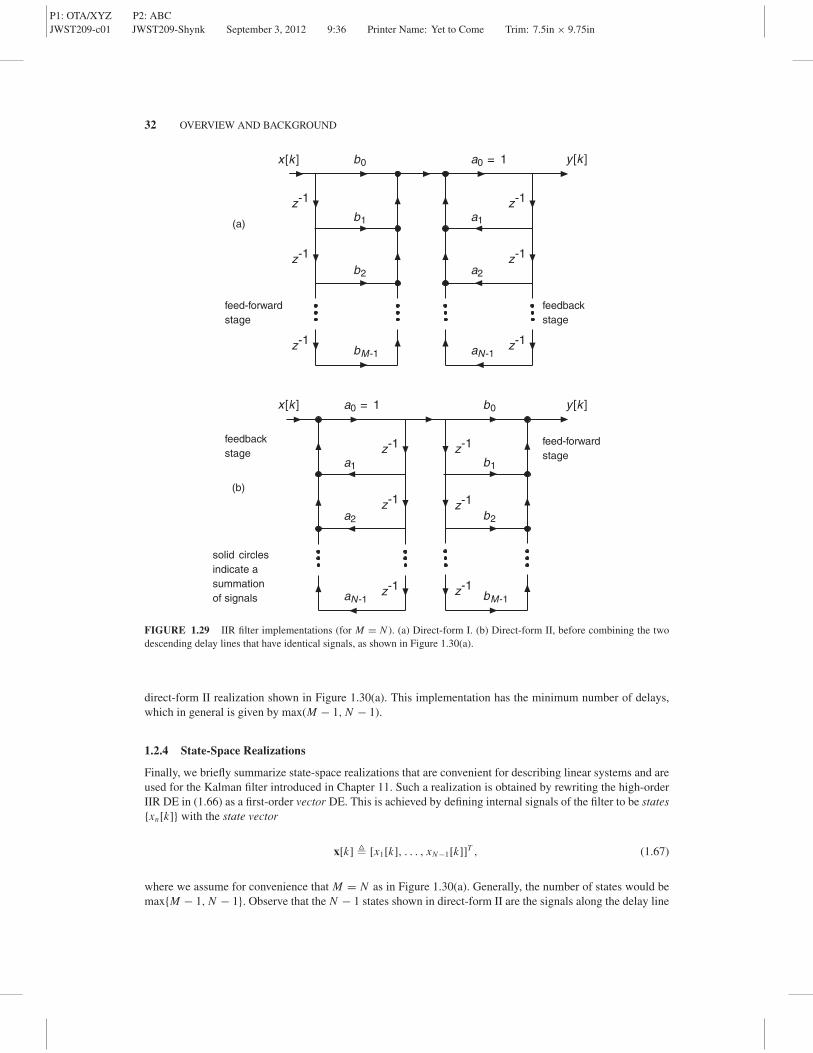
where a0 = 1 has been assumed. Examples of IIR filter implementations are shown in Figure 1.29. There areseveral IIR implementations; the one shown in Figure 1.29(a) is called direct-form I and corresponds to a directrealization of the DE in (1.66). Since the filter is LTI, the feed-forward and feedback stages can be interchanged,leading to the second structure in Figure 1.29(b). Observe that in this configuration, the two sets of delayedsignals are identical, and thus the two delay lines can be combined into a single delay line, resulting in the
P1: OTA/XYZ P2: ABCJWST209-c01 JWST209-Shynk September 3, 2012 9:36 Printer Name: Yet to Come Trim: 7.5in × 9.75in
32 OVERVIEW AND BACKGROUND
solid circlesindicate a summationof signals
(a)
(b)
y [k ]
a1
aN -1
a2
z-1
z-1
z-1
x [k ] b0
b1
b2
bM -1
z-1
z-1
z-1
a0 = 1
x [k ] b0
b1
b2
bM -1
z-1
z-1
z-1
y [k ]
a1
aN -1
a2
z-1
z-1
z-1
a0 = 1
feed-forwardstage
feedbackstage
feed-forwardstage
feedbackstage
FIGURE 1.29 IIR filter implementations (for M = N ). (a) Direct-form I. (b) Direct-form II, before combining the twodescending delay lines that have identical signals, as shown in Figure 1.30(a).
direct-form II realization shown in Figure 1.30(a). This implementation has the minimum number of delays,which in general is given by max(M − 1, N − 1).
1.2.4 State-Space Realizations
Finally, we briefly summarize state-space realizations that are convenient for describing linear systems and areused for the Kalman filter introduced in Chapter 11. Such a realization is obtained by rewriting the high-orderIIR DE in (1.66) as a first-order vector DE. This is achieved by defining internal signals of the filter to be states{xn[k]} with the state vector
x[k] � [x1[k], . . . , xN−1[k]]T , (1.67)
where we assume for convenience that M = N as in Figure 1.30(a). Generally, the number of states would bemax{M − 1, N − 1}. Observe that the N − 1 states shown in direct-form II are the signals along the delay line

P1: OTA/XYZ P2: ABCJWST209-c01 JWST209-Shynk September 3, 2012 9:36 Printer Name: Yet to Come Trim: 7.5in × 9.75in
DETERMINISTIC SIGNALS AND SYSTEMS 33
(a) x1[k ]
[k ]x2
x
z-1
z-1
z-1
a1
a
a2
a0 = 1 b0
b1
b2
bM -1
(b)
x1
x2[k ]
[k ]xN -1
N -1
M -1 N-1
N -1[k ]
z-1
z-1
z-1
b1
b
b2
b0 a0 = 1
a1
a2
a
solid circlesindicate asummationof signals
x [k ]
x [k ]
y [k ]
y [k ]
[k ]
FIGURE 1.30 IIR filter implementations (for M = N ). (a) Direct-form II (after combining the two descending delay linesin Figure 1.29(b)) with state signals defined. (b) Alternative realization with ascending delay line and different state signalsdefined.
so that we can write the following system of equations:
x1[k + 1] =N−1∑
n=1
an xn[k] + x[k],
x2[k + 1] = x1[k],
...
xN−1[k + 1] = xN−2[k]. (1.68)
From the state-vector definition, this leads to the following vector recursion:
x[k + 1] = Ax[k] + bx[k], (1.69)

P1: OTA/XYZ P2: ABCJWST209-c01 JWST209-Shynk September 3, 2012 9:36 Printer Name: Yet to Come Trim: 7.5in × 9.75in
34 OVERVIEW AND BACKGROUND
where
A �
⎡
⎢⎢⎢⎢⎢⎢⎢⎢⎢⎢⎢⎣
a1 a2 · · · aN−1
1 0 · · · 0
0 1 0 · · ·...
.... . .
. . ....
0 · · · 0 1 0
⎤
⎥⎥⎥⎥⎥⎥⎥⎥⎥⎥⎥⎦
, b �
⎡
⎢⎢⎢⎣
10...0
⎤
⎥⎥⎥⎦ . (1.70)
The DE can be rewritten in terms of the states as follows (again, with M = N ):
y[k] =M−1∑
m=1
bm xm[k] + b0
N−1∑
n=1
an xn[k] + b0x[k], (1.71)
=N−1∑
n=1
(bn + b0an)xn[k] + b0x[k], (1.72)
and thus the output is
y[k] = cT x[k] + dx[k], (1.73)
where
c � [b1 + b0a1, . . . , bN−1 + b0aN−1]T , d = b0. (1.74)
Equations (1.69) and (1.73) together comprise the state-space formulation for the direct-form II filter withparameters {A, b, c, d}.
Other state-space forms can be obtained by rearranging the direct-form II realization. For example, in-terchanging x[k] and y[k], reversing the directions of all arrows, interchanging nodes and summations, andreversing the diagram horizontally results in the “dual” realization shown in Figure 1.30(b). The two realizationsin the figure have identical transfer functions (poles and zeros), but different state-space representations. Notein Figure 1.30(b) that we have again labeled the states to be at the output of the delays. The corresponding stateequations are (with M = N )
x1[k + 1] = b1x[k] + a1 y[k] + x2[k],
...
xN−2[k + 1] = bN−2x[k] + aN−2 y[k] + xN−1[k],
xN−1[k + 1] = bN−1x[k] + aN−1 y[k]. (1.75)
Substituting y[k] = x1[k] + b0x[k] gives
x1[k + 1] = (b1 + b0a1)x[k] + a1x1[k] + x2[k],
...
xN−2[k + 1] = (bN−2 + b0aN−2)x[k] + aN−2xN−2[k] + xN−1[k],
xN−1[k + 1] = (bN−1 + b0aN−1)x[k] + aN−1xN−1[k], (1.76)

P1: OTA/XYZ P2: ABCJWST209-c01 JWST209-Shynk September 3, 2012 9:36 Printer Name: Yet to Come Trim: 7.5in × 9.75in
STATISTICAL SIGNAL PROCESSING WITH MATLAB® 35
and thus the state-space parameters are
A �
⎡
⎢⎢⎢⎢⎢⎢⎢⎢⎢⎢⎢⎣
a1 1 0 · · · 0
a2 0 1...
.... . .
. . . 0
· · · 0 1
aN−1 0 · · · 0
⎤
⎥⎥⎥⎥⎥⎥⎥⎥⎥⎥⎥⎦
, b �
⎡
⎢⎣b1 + b0a1
...bN−1 + b0aN−1
⎤
⎥⎦ , (1.77)
c � [1, 0, . . . , 0]T , d = b0. (1.78)
Note that state transition matrix A for this dual realization is the transpose of that in (1.70), b and c areinterchanged, and d remains the same scalar b0.
1.3 STATISTICAL SIGNAL PROCESSING WITH MATLAB®
Although continuous-time random processes and discrete-time random sequences are covered in this book, allsimulation examples generated using MATLAB®1 are necessarily discrete-time sequences. In this section, weprovide an overview of methods for generating random sequences, and of filters for modifying their propertiesand frequency-domain characteristics.
1.3.1 Random Number Generation
The random number generators in MATLAB provide a means for realizing a pseudorandom sequence X [k]where the samples across time instants are independent and thus uncorrelated. There are two basic randomnumber generators:
1. randn(N,1). Generates an N × 1 vector of numbers on R from the standard Gaussian distribution withzero mean and unit variance.
2. rand(N,1). Generates an N × 1 vector of numbers from the continuous uniform distribution on [0, 1].
Example histograms with N = 2000 samples for the two random number generators are shown in Figure 1.31,where n is the number of samples in a particular bin along the x-axis. By decreasing the bin width and increasingthe number of samples, these histograms approach the pdfs:
fX (x) = 1√2π
exp(−x2/2) (standard Gaussian), (1.79)
fX (x) = I[0,1](x) (uniform on unit interval), (1.80)
where I(x) is the indicator function (see Appendix B). However, even for an infinite number of samples, thehistograms and the random number generators are still only an approximation because it is not possible togenerate all real numbers due to finite-precision arithmetic used in a computer.
1MATLAB is a registered trademark of The Mathworks, Inc., 3 Apple Hill Drive, Natick, MA.

P1: OTA/XYZ P2: ABCJWST209-c01 JWST209-Shynk September 3, 2012 9:36 Printer Name: Yet to Come Trim: 7.5in × 9.75in
36 OVERVIEW AND BACKGROUND
–4 –3 –2 –1 0 1 2 3 40
10
20
30
40
50
60
70
80
90
100
x
n
Histogram of Gaussian Samples(a)
(b)
0 0.2 0.4 0.6 0.8 10
5
10
15
20
25
30
35
40
45
50
x
n
Histogram of Uniform Samples
FIGURE 1.31 Histograms for two random number generators in MATLAB (2000 samples). (a) Standard Gaussian.(b) Uniform on [0, 1].
In the event that we want to change the mean and variance for the Gaussian random number generator, therandom sequence is modified as follows:
Y [k] = σY X [k] + μY . (1.81)
Sequence Y [k] also has a Gaussian distribution, but with mean μY and variance σ 2Y . Note that X [k] is multiplied
by σY first, and then μY is added; σY (X [k] + μY ) does not produce the same result. Examples of randomsequences generated by rand and randn are shown in Figure 1.32. Obviously the Gaussian realization hasgreater range than the uniform realization whose values are restricted to be ∈ [0, 1]. The sample at each timeinstant is independent of all other samples; generating correlated sequences using MATLAB is covered later inChapter 5.

P1: OTA/XYZ P2: ABCJWST209-c01 JWST209-Shynk September 3, 2012 9:36 Printer Name: Yet to Come Trim: 7.5in × 9.75in
STATISTICAL SIGNAL PROCESSING WITH MATLAB® 37
200 400 600 800 1000 1200 1400 1600 1800 2000
–3
–2
–1
0
1
2
3
k
x[k
]x
[k]
Gaussian Realization(a)
(b)
200 400 600 800 1000 1200 1400 1600 1800 20000
0.2
0.4
0.6
0.8
1
k
Uniform Realization
FIGURE 1.32 Example realizations of uncorrelated random sequences. (a) Standard Gaussian. (b) Uniform on [0, 1].
Random generator randn is useful because Gaussian processes arise often in practice, such as noise in acommunication system. It is relatively easy to transform from one random variable to another, and this is moreeasily done starting with rand. If X is a uniform random variable with support [0, 1], and FY (y) is the cdf ofthe desired random variable Y , then using the transformation techniques in Chapter 4, it is easily shown that Yis obtained as follows:
Y = F−1Y (X ), (1.82)
where F−1Y (·) is the inverse image of the cdf. The cdf and inverse cdf (icdf) for the standard Gaussian random
variable are shown in Figure 1.33. In a computer simulation, a sample of X would be generated using rand,

P1: OTA/XYZ P2: ABCJWST209-c01 JWST209-Shynk September 3, 2012 9:36 Printer Name: Yet to Come Trim: 7.5in × 9.75in
38 OVERVIEW AND BACKGROUND
−4 −3 −2 −1 0 1 2 3 4
−2
−1.5
−1
−0.5
0
0.5
1
1.5
2
x
FX
(x),
FX−
1 (x)
Gaussian Cdf and Icdf
cdficdf
FIGURE 1.33 Gaussian cdf and icdf.
and then it would be transformed to Y via (1.82). Observe in Figure 1.33 that the range of X for the icdf isthe support [0, 1] of rand. This is not a coincidence. As discussed in Chapter 3, the cdf of Y is the followingprobability:
FY (y) � P(Y ≤ y), (1.83)
and thus FY (y) ∈ [0, 1] by the axioms of probability (this is seen in Figure 1.33). The support of FY (y) isR, although some random variables have finite support, so that FY (y) is either zero or one before or aftersome finite value (as is the case for the uniform random variable). The range of the icdf is, in general, theentire real line as implied by the curve in Figure 1.33. The interval for rand has been chosen specifically tobe uniform on [0, 1] so that it exactly matches the range of a cdf. Mapping rand samples via the icdf givesthe corresponding samples on R for the random variable defined by the particular icdf. However, note thatMATLAB has random number generators for many of the distributions covered in this book. These randomnumber generators are implemented using random(“type,” “parameters”) where “type” is the name of therandom variable, and “parameters” is a list of the specific values of the pdf parameters (location, scale, shape,degrees of freedom, or threshold).
1.3.2 Filtering
There are two basic functions for filtering sequences in MATLAB:
� filter(b, a, x): generates an output vector that is the same size as the input vector x, where a �[a0, . . . , aN−1]T and b � [b0, . . . , bM−1]T contain the filter coefficients of the linear DE in (1.66). Thedirect-form II configuration in Figure 1.30(a) is used.
� conv(h, x): generates a 2N − 1 output vector realizing the convolution in (1.47), but with summationrange {0, . . . , N − 1} and for finite-length coefficient vector h = [h[0], . . . , h[N − 1]]T and input vectorx = [x[k], . . . , x[k − N + 1]]T .

P1: OTA/XYZ P2: ABCJWST209-c01 JWST209-Shynk September 3, 2012 9:36 Printer Name: Yet to Come Trim: 7.5in × 9.75in
PROBLEMS 39
200 400 600 800 1000 1200 1400 1600 1800 2000
−1
−0.5
0
0.5
1
k
y[k
]
Filter Output
FIGURE 1.34 Example filter output realization of the Gaussian random sequence in Figure 1.32(a).
An FIR filter is realized using filter by setting a = 1. conv also implements an FIR filter, but differs from filterbecause its output extends beyond the length of the input vector x. This is achieved by assuming that values ofx[k] not contained in x are zero. As a result, filter is preferred in most filtering applications. An example of anFIR filter using filter(b, a, x) operating on the sequence in Figure 1.32(a) with b = (1/10)[1, . . . , 1]T ∈ R10
and a = 1 is shown in Figure 1.34. This filter has a low-pass frequency response, which we see yields an outputthat is less “noisy” than the input; the output sequence is correlated.
PROBLEMS
Delta Functions
1.1 (a) Find the area of g(x) on [−1, 2.5]:
g(x) = 5δ(x) + 3δ(x − 2) − 2δ(x − 3). (1.84)
(b) Find a general expression for h(x) on R+ = [0, ∞):
h(x) =∫ x
−∞g(u)du. (1.85)
1.2 (a) Convolve the following functions:
g(x) =3∑
n=1
2nδ(x − n), h(x) = exp(−x)u(x). (1.86)
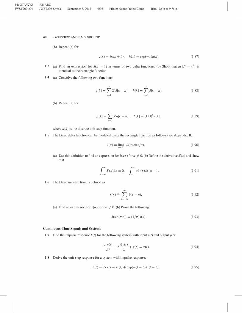
P1: OTA/XYZ P2: ABCJWST209-c01 JWST209-Shynk September 3, 2012 9:36 Printer Name: Yet to Come Trim: 7.5in × 9.75in
40 OVERVIEW AND BACKGROUND
(b) Repeat (a) for
g(x) = δ(ax + b), h(x) = exp(−x)u(x). (1.87)
1.3 (a) Find an expression for δ(x2 − 1) in terms of two delta functions. (b) Show that u(1/4 − x2) isidentical to the rectangle function.
1.4 (a) Convolve the following two functions:
g[k] =3∑
n=1
2nδ[k − n], h[k] =2∑
n=1
δ[k − n]. (1.88)
(b) Repeat (a) for
g[k] =1∑
n=0
3nδ[k − n], h[k] = (1/3)ku[k], (1.89)
where u[k] is the discrete unit-step function.
1.5 The Dirac delta function can be modeled using the rectangle function as follows (see Appendix B):
δ(x) = lima→0
(1/a)rect(x/a). (1.90)
(a) Use this definition to find an expression for δ(αx) for α = 0. (b) Define the derivative δ′(x) and showthat
∫ ∞
−∞δ′(x)dx = 0,
∫ ∞
−∞xδ′(x)dx = −1. (1.91)
1.6 The Dirac impulse train is defined as
s(x) �∞∑
n=−∞δ(x − n). (1.92)
(a) Find an expression for s(αx) for α = 0. (b) Prove the following:
δ(sin(πx)) = (1/π )s(x). (1.93)
Continuous-Time Signals and Systems
1.7 Find the impulse response h(t) for the following system with input x(t) and output y(t):
d2 y(t)
dt2+ 2
dy(t)
dt+ y(t) = x(t). (1.94)
1.8 Derive the unit-step response for a system with impulse response:
h(t) = 2 exp(−t)u(t) + exp(−(t − 5))u(t − 5). (1.95)

P1: OTA/XYZ P2: ABCJWST209-c01 JWST209-Shynk September 3, 2012 9:36 Printer Name: Yet to Come Trim: 7.5in × 9.75in
PROBLEMS 41
1.9 Find Laplace transforms for the following signals and specify their ROCs:
x1(t) = exp(−5|t |), x2(t) = erf(t)u(t), (1.96)
where erf(t) is the error function.
1.10 Repeat Problem 1.9 for
x1(t) = rect(t), x2(t) = 1/t, (1.97)
1.11 Repeat Problem 1.9 for
x1(t) = t exp(−3t)u(t − 1), x2(t) = cos(2π t − 5)u(t − 2). (1.98)
1.12 From a PFE find the inverse Laplace transform for
H (s) = 2s
s2 + 3s + 2, (1.99)
which has ROC Re(s) > −1.
1.13 Repeat Problem 1.12 for
H (s) = 2s
s2 − s − 2, (1.100)
which has ROC −1 < Re(s) < 2.
1.14 Convolve the following two functions:
x(t) = exp(−2t)u(t) + exp(−t + 1)u(t − 1), h(t) = u(t − 2). (1.101)
1.15 Find the output y(t) of the following system:
dy(t)
dt+ 4y(t) = x(t) (1.102)
for x(t) = exp(−t)u(t − 1).
1.16 The deterministic cross-correlation is computed as follows:
y(t) =∫ ∞
−∞x(τ )h(t + τ )dτ. (1.103)
(a) Derive an expression for Y (ω) in terms of X (ω) and H (ω). (a) Compute the cross-correlation functionfor the functions in Problem 1.14.
1.17 Prove Parseval’s theorem for real-valued x(t):
∫ ∞
−∞x2(t)dt =
∫ ∞
−∞|X ( f )|2d f. (1.104)
1.18 Find Fourier transforms for the following functions:
x1(t) = 5rect(5t), x2(t) = exp(−|t |) cos(4π t). (1.105)

P1: OTA/XYZ P2: ABCJWST209-c01 JWST209-Shynk September 3, 2012 9:36 Printer Name: Yet to Come Trim: 7.5in × 9.75in
42 OVERVIEW AND BACKGROUND
1.19 Determine the frequency response Y (ω) for
y(t) = 1
π
∫ ∞
−∞
x(τ )
t − τdτ. (1.106)
Discrete-Time Signals and Systems
1.20 Find the impulse response h[k] for the following system with input x[k] and output y[k]:
y[k] + 2y[k − 1] + 4y[k − 2] = x[k] + 2x[k − 1]. (1.107)
1.21 Find the unit-step response for a system with impulse response:
h[k] = (1/3)ku[k] − 2u[k − 1]. (1.108)
1.22 Determine the z-transform for the following signals and specify their ROCs:
x1[k] = (k − 1)2u[k − 1], x2[k] = (1/2)ku[k] + 4ku[k + 1]. (1.109)
1.23 Repeat Problem 1.22 for
x1[k] = 3ku[−k + 1], x2[k] = 2u[k] − 2u[k − 5]. (1.110)
1.24 Find DTFTs for the following signals:
x1[k] = sinc[k − 1], x2[k] = k(1/2)k−1u[k]. (1.111)
1.25 Consider the sample mean
x̄[k] = 1
k
k∑
n=0
x[n]. (1.112)
(a) Specify the zeros of this system for k = 2. (b) Rewrite x̄[k] in recursive form in terms of x̄[k − 1]and sketch a digital filter implementation.
1.26 Convolve the following two functions:
x[k] = ak−1 IN [k], h[k] = u[k] − u[k − N ], (1.113)
where I{a,b}[k] is the discrete indicator function and N = {1, 2, . . .} are the natural numbers.
1.27 The deterministic cross-correlation function is given by
y[k] =∞∑
n=−∞x[n]h[k + n]. (1.114)
Find the cross-correlation of the two functions in Problem 1.26.
1.28 Prove the derivative property of the z-transform: kx[k] → −zdX (z)/dz.

P1: OTA/XYZ P2: ABCJWST209-c01 JWST209-Shynk September 3, 2012 9:36 Printer Name: Yet to Come Trim: 7.5in × 9.75in
PROBLEMS 43
1.29 Find the inverse z-transform for
H (z) = 2(z + 1)
(z + 1/2)(z − 1/3)(1.115)
using Cauchy’s residue theorem (see Appendix C) when the ROC is |z| > 1/2.
1.30 Repeat Problem 1.29 when the ROC is 1/3 < |z| < 1/2.
1.31 Use Cauchy’s residue theorem to find the inverse z-transform of the following transfer function such thath[k] is a left-sided impulse response function:
H (z) = 3
(z + 1/2)(3/2 − z). (1.116)
1.32 Find expressions for the magnitude and phase of the DTFT H ( jω) for
H (z) = 5z
(z − 1/4)(z + 1/5). (1.117)
1.33 Repeat Problem 1.32 for the following finite-length sequence:
x[k] = exp( jωok)I{0,...,N−1}[k]. (1.118)
Sampling of Continuous-Time Signals
1.34 The continuous-time signal x(t) = exp(−αt)u(t) is uniformly sampled with sampling period Ts : xs(t) =x(t)s(t), where s(t) is the ideal impulse train in (1.43). (a) Find an expression for Xs(ω) showing thatX (ω) is repeated at integer multiples of 2π/Ts . (b) Derive the DTFT X ( jω) of the sampled signal x[kTs]and demonstrate that there is aliasing by comparing it to Xs(ω).
1.35 Instead of using the ideal impulse train, consider sampling x(t) with the following rectangular pulsetrain:
p(t) =∞∑
n=−∞rect(t/Tp − nTs), (1.119)
where Tp � Ts . The Fourier series of p(t) is
p(t) =∞∑
m=−∞pm exp( j2πmt/Ts) (1.120)
with
pm = 1
Ts
∫ Tp
−Tp
exp(− j2πmt/Ts)dt. (1.121)
Find a closed-form representation for pm and use it to write an expression for the sampled waveformx p(t) = x(t)p(t) and its Fourier transform X p(ω).
1.36 Consider the following continuous-time signal:
x(t) = 2 cos(200π t) + 4 cos(400π t) + 3 cos(600π t). (1.122)

P1: OTA/XYZ P2: ABCJWST209-c01 JWST209-Shynk September 3, 2012 9:36 Printer Name: Yet to Come Trim: 7.5in × 9.75in
44 OVERVIEW AND BACKGROUND
Let x(t) be sampled using an ideal impulse train s(t) to generate the sampled waveform xs(t). Find andsketch the Fourier transform of xs(t) for the following sampling rates. (a) fs = 300 Hz. (b) fs = 500Hz. Comment about any aliasing that might occur.
1.37 The ideal reconstruction filter has frequency response:
H (ω) = Tsrect(ω/2W ) ={
Ts, |ω| ≤ W0, else,
(1.123)
where W is the one-sided bandwidth of the sampled waveform x(t). The Fourier transform of the originalwaveform is obtained as X (ω) = H (ω)Xs(ω) assuming that the Nyquist rate is satisfied: fs = 1/Ts >
2W . Find an expression for x(t) as a convolution of the samples {x(kTs)} and the impulse response h(t)of H (ω).
Discrete-Time Filters
1.38 A discrete-time system has the following transfer function:
H (z) = 5(z − 2)
(z − 0.3)(z2 + 0.1z − 0.6). (1.124)
(a) Find and sketch the direct-form I and direct-form II filter structures. (b) Using a PFE and a productof first-order sections, respectively, find and sketch parallel and cascade filter structures.
1.39 Repeat Problem 1.38 for
H (z) = 2(z2 − (5/6)z + 1/6)
(z + 1/2)(z2 − 1/16). (1.125)
1.40 A discrete-time filter has impulse response:
h[k] = (0.8)ku[k] + (−0.4)k−1u[k − 1]. (1.126)
(a) Derive and sketch a direct-form II implementation for this filter. (b) Write the output y[k] as adifference equation with input x[k].
1.41 Consider the following system:
H (z) = z + 2
(z2 − (1/12)z − 1/12)(z + 1/2). (1.127)
(a) Write a difference equation for the output y[k] in terms of the input x[k]. (b) Derive the parameters{A, b, c, d} for the state-space realization defined by (1.68). (c) Repeat part (b) for the state-spacerealization defined by (1.75).
1.42 Repeat Problem 1.41 for the system in (1.124).
Computer Problems
1.43 Generate N = 1000 samples using randn and plot the resulting Gaussian sequence x[k]. Process x[k]to generate output y[k] using a filter with the following transfer function:
H (z) = 2
z − p. (1.128)

P1: OTA/XYZ P2: ABCJWST209-c01 JWST209-Shynk September 3, 2012 9:36 Printer Name: Yet to Come Trim: 7.5in × 9.75in
FURTHER READING 45
Use filter and several different values of p.
1.44 Generate N = 1000 samples using rand and plot the uniformly distributed random sequence x[k].Convert x[k] to an exponential random sequence with parameter λ using the appropriate icdf in MATLAB.Comment about the range of outcomes of the sequences for different parameter values: (a) λ = 1 and(b) λ = 0.1.
1.45 Use randn to generate 10 samples of a Gaussian random variable, map them to ±1 via the sign function,and then insert a zero in between each bit using upsample, resulting in a sequence of 20 symbolsconsisting of 0s and ±1s. Use rectpulse to map each symbol to a rectangle function of duration 100samples, and plot the resulting PAM waveform using stairs.
FURTHER READING
The topics on signals and systems reviewed at the end of this chapter can be explored further in the followingreferences. Dirac delta function: Bracewell (1978) and Weisstein (2003). Continuous-time linear systems:Lathi (1965), Lathi (2000), and Oppenheim, Willsky, and Nawab (1996). Digital signal processing: Hamming(1983), Oppenheim and Schafer (2009), Mitra (2010), Rabiner and Gold (1975), and Stearns and Hush (1990).State-space formulations: Kailath (1980), Mendel (1995), and Tretter (1976). Signal processing with MATLAB:Chaparro (2011), Childers (1997), Ingle and Proakis (2011), and McClellan, Schafer, and Yoder (1998).

P1: OTA/XYZ P2: ABCJWST209-c01 JWST209-Shynk September 3, 2012 9:36 Printer Name: Yet to Come Trim: 7.5in × 9.75in
46