1 on the use of greedy shapers in real-time … · shaper to conform again to the input trafﬁc...

1

On the Use of Greedy Shapers in Real-Time Embedded Systems

ERNESTO WANDELER, ALEXANDER MAXIAGUINE, and LOTHAR THIELE, ETH Zurich

Traffic shaping is a well-known technique in the area of networking and is proven to reduce global bufferrequirements and end-to-end delays in networked systems. Due to these properties, shapers also play anincreasingly important role in the design of multiprocessor embedded systems that exhibit a considerableamount of on-chip traffic. Despite the growing importance of traffic shapping in this area, no methodsexist for analyzing shapers in distributed embedded systems and for incorporating them into a system-level performance analysis. Until now it was not possible to determine the effect of shapers on end-to-enddelay guarantees or buffer requirements in such systems. In this work, we present a method for analyzinggreedy shapers, and we embed this analysis method into a well-established modular performance analysisframework for real-time embedded systems. The presented approach enables system-level performanceanalysis of complete systems with greedy shapers, and we prove its applicability by analyzing three casestudy systems.

Categories and Subject Descriptors: C.3 [Computer System Organization]: Special Purpose andApplication-Based Systems—Real-time and embedded systems

General Terms: Design, Performance, Verification

Additional Key Words and Phrases: Embedded systems, performance analysis, shapers

ACM Reference Format:Wandeler, E., Maxiaguine, A., and Thiele, L. 2012. On the use of greedy shapers in real-time embeddedsystems. ACM Trans. Embedd. Comput. Syst. 11, 1, Article 1 (March 2012), 22 pages.DOI = 10.1145/2146417.2146418 http://doi.acm.org/10.1145/2146417.2146418

1. INTRODUCTION

In the area of broadband networking, traffic shaping is a well-known and well-studiedtechnique for regulating connections and avoiding buffer overflow in network nodes,see, for example, Gringeri et al. [1998] or Rexford et al. [1997]. A traffic shaper in anetwork node buffers the data packets of an incoming traffic stream and delays themsuch that the output stream conforms to a given traffic specification. A shaper mayensure, for example, that the output stream has limited burstiness or that packetson the output stream have a specified minimum interarrival time. A greedy shaperis a special instance of a traffic shaper that not only ensures an output stream thatconforms to a given traffic specification but also guarantees that no packets get delayedlonger than necessary.

Non-greedy shapers are able to keep packets longer than necessary in order tosmoothen the output traffic. For example, besides a maximal number of output packetsin a given time interval, one may also specify a minimal number in order to avoid a

This research has been funded by the Swiss National Science Foundation (SNF) under the Analytic Perfor-mance Estimation of Embedded Computer Systems project 200021-103580/1 and by ARTIST2.Authors’ addresses: E. Wandeler, A. Maxiaguine, and L. Thiele, Computer Engineering and Networks Lab-oratory, Swiss Federal Institute of Technology (ETH), CH-8092 Zurich, Switzerland; corresponding author’semail: [email protected] to make digital or hard copies of part or all of this work for personal or classroom use is grantedwithout fee provided that copies are not made or distributed for profit or commercial advantage and thatcopies show this notice on the first page or initial screen of a display along with the full citation. Copyrights forcomponents of this work owned by others than ACM must be honored. Abstracting with credit is permitted.To copy otherwise, to republish, to post on servers, to redistribute to lists, or to use any component of thiswork in other works requires prior specific permission and/or a fee. Permissions may be requested fromPublications Dept., ACM, Inc., 2 Penn Plaza, Suite 701, New York, NY 10121-0701 USA, fax +1 (212)869-0481, or [email protected]© 2012 ACM 1539-9087/2012/03-ART1 $10.00

DOI 10.1145/2146417.2146418 http://doi.acm.org/10.1145/2146417.2146418

ACM Transactions on Embedded Computing Systems, Vol. 11, No. 1, Article 1, Publication date: March 2012.

1:2 E. Wandeler et al.

SharedBUS

CNI1

External InputShaping

CPU1

TS1 σ1S1’ S1’’S1

CNI2CPU2

TS2 σ2S2’ S2’’S2

CNI3

CNI4

S1’’’

S2’’’

CPU1

TS1S1’’S1 σ1

TS2S2’’S2 σ2

TS3S3’’S3 σ3

S1’

S2’

S3’

MPSoC

Internal Reshaping

Fig. 1. Two systems with greedy shapers.

buffer underflow or to get a smoother output traffic. Therefore, shaping devices withthis property are sometimes called smoothers. They may keep a number of packets as areserve and send them in case of low input traffic. This way, a violation of the specifiedminimal packet rate can be avoided. This article concentrates on greedy shapers.

By limiting the burstiness of the output stream of a network node, shapers typicallydrastically reduce the buffer requirements on subsequent network nodes. In particular,if some sort of priority scheduling is used on a network node to share bandwidth amongseveral incoming streams, then a limited burstiness of high-priority streams leads tobetter responsiveness of low-priority streams.

In addition, under some circumstances, shaping comes for free from a performancepoint of view. To be more specific, if the output stream of a node is shaped with a greedyshaper to conform again to the input traffic specification, and if the buffer of the shaperaccesses the same memory as the input buffer of the node, then the end-to-end delayof the stream and the total buffer requirements on the network node are not affectedby adding the shaper.

Due to these favorable properties, shapers also play an increasingly important rolein the design of real-time embedded systems. Modern embedded systems are oftenimplemented as multiprocessor systems with a considerable amount of on-chip traffic.

In this domain, we may identify two main application areas for traffic shaping.First, shapers may be used internally to reshape internal traffic streams to reduceglobal buffer requirements and end-to-end delays. Second, shapers may be added atthe boundaries of a system to ensure conformant input streams, thereby preventinginternal buffer overflows caused by malicious input. Figure 1 shows two simple examplesystems from these two application areas.

Within the framework of Network Calculus Le Boudec and Thiran [2001] presentmethods for analyzing the effects of traffic shapers in communication networks. Butto our best knowledge, none of the existing frameworks for modular system-level per-formance analysis of real-time embedded system considers traffic shapers at this time,see, for example, Pop et al. [2003], Richter et al. [2003], Gonzalez Harbour et al. [2001]or Chakraborty et al. [2003], or Thiele et al. [2000].

Only Richter et al. [2003] introduce a restricted kind of traffic shaping throughso-called event adaption functions (EAFs). However, EAF’s play a crucial role in themethod’s fundamental ability to analyze systems, and therefore, a designer has verylimited freedom to place or omit or parameterize EAF’s.


On the Use of Greedy Shapers in Real-Time Embedded Systems 1:3

In this work, we will extend the framework presented in Chakraborty et al. [2003] andThiele et al. [2000] to enable system-level performance analysis of real-time embeddedsystems with traffic shapers. The first (and preliminary) results on greedy shapershave been published in Wandeler et al. [2006]. It has to be noted that Le Boudec andThiran [2001] challenge the ability of the methods presented by Thiele et al. [2000] toanalyze traffic shapers, Schioler et al. [2005] even claim that it is not possible to analyzetraffic shapers within the framework of modular performance analysis [Chakrabortyet al. 2003; Thiele et al. 2000]. This article proposes a solution to these problems andchallenges.

The contributions of this work can be summarized as follows.

—We present a method for analyzing greedy shapers in multiprocessor embeddedsystems.

—We embed this new analysis method into the well-established modular performanceanalysis framework of Chakraborty et al. [2003] and Thiele et al. [2000]. This enablessystem-level performance analysis of complete systems with greedy shapers, that is,we may analyze end-to-end delay guarantees and global buffer requirements of suchsystems.

—We prove the applicability of the presented methods by analyzing two small casestudy systems with greedy shapers.

2. MODULAR PERFORMANCE ANALYSIS

In the domain of communication networks, powerful abstractions have been developedto model flow of data through a network. In particular, Network Calculus [Cruz 1991]provides a means to deterministically reason about timing properties of data flows inqueuing networks. Real-Time Calculus [Thiele et al. 2000] extends the basic concepts ofNetwork Calculus to the domain of real-time embedded systems, and Chakraborty et al.[2003] proposes a unifying approach to Modular Performance Analysis with Real-TimeCalculus. It is based on a general event and resource model, allows for hierarchicalscheduling and arbitration, and takes computation and communication resources intoaccount.

With Real-Time Calculus, hard upper and lower bounds can be computed to vari-ous performance measures in a real-time system, such as end-to-end delays of eventstreams or buffer requirements. Hence, real-Time Calculus qualifies to analyze hardreal-time systems. This clearly distinguishes Real-Time Calculus from any probabilisticperformance estimation methods or from performance estimation through simulation.

The central idea of Modular Performance Analysis is to first build an abstract per-formance model of the concrete system that bundles all information needed for per-formance analysis with Real-Time Calculus. The abstract performance model therebyunifies essential information the environment of the system, the available computa-tion and communication resources, the application tasks (or dedicated HW/SW compo-nents), as well as the system architecture itself.

Within the abstract performance model, environment models describe how a systemis being used by the environment: how often events (or function calls) will arrive; howmuch data is provided as input to the system; and how many events and how muchdata is generated in return by the system and fed back to the environment. Resourcemodels provide information about the properties of the computing and communicationresources that are available within a system, such as processor speed and communica-tion bus bandwidth. Application task (or dedicated HW/SW component) models provideinformation about the processing semantics that is then used to execute the variousapplication tasks or run the dedicated HW/SW components. Finally, the system modelcaptures information about the applications and the available hardware architecture,



defines the mapping of tasks to computation or communication resources of the hard-ware architecture, and specifies the scheduling and arbitration schemes used on theseresources.

Following, we introduce the basic concepts of Network and Real-Time Calculus.

2.1. Arrival Curves: A General Event Stream Model

A trace of an event stream can be described by means of a cumulative function R(s, t),defined as the number of events seen on the event stream in the time interval [s, t).While any R always describes one concrete trace of an event stream, a tuple α(�) =[αu(�), αl(�)] of upper and lower arrival curves [Cruz 1991] provides an abstract eventstream model, representing all possible traces of an event stream.

The upper arrival curve αu(�) provides an upper bound on the number of eventsseen on the event stream in any time interval of length �, and analogously, the lowerarrival curve αl(�) denotes a lower bound on the number of events in a time interval�. R, αu and αl are related to each other such that

αl(t − s) ≤ R(s, t) ≤ αu(t − s) ∀s < t, (1)

with αl(0) = αu(0) = 0.Arrival curves substantially generalize traditional event models, for example, as

sporadic, periodic, periodic with jitter, or any other arrival pattern with determinis-tic timing behavior. For example, an event stream with a period p, a jitter j, and aminimum inter-arrival distance d can be modeled by the following arrival curves.

αl(�) =⌊

� − jp

⌋; αu(�) = min

{⌈� + j

p

⌉,

⌈�

d

⌉}. (2)

Besides being able to represent any message stream with known deterministic timingbehavior, it is also possible to determine arrival curves corresponding to any finite-length message trace, obtained, for example, from observation or simulation.

Figure 2 shows some typical examples of arrival curves. The arrival curves inFigure 2(a) model a strictly periodic event stream, while the arrival curves inFigure 2(b) model a periodic event stream with jitter, and the arrival curvesin Figure 2(c) model a periodic event stream with bursts. The arrival curves inFigure 2(d) model an event stream with more complex timing behavior. This eventstream may have short steep bursts or longer-lasting less steep bursts, and themaximum long-term period does not equal the minimum long-term period. An eventstream with such a complex timing behavior can not be represented accurately by anyof the classical event arrival patterns.

2.2. Service Curves: A General Resource Model

Analogously to the cumulative function R(s, t), the concrete availability of a compu-tation or communication resource can be described by a cumulative function C(s, t),defined as the number of available resources, for example, processor or bus cycles,in the time interval [s, t). To provide an abstract resource model, we define a tupleβ(�) = [βu(�), βl(�)] of upper, βu and lower βl, service curves. C, βu, and βl are relatedto each other such that

βl(t − s) ≤ C(s, t) ≤ βu(t − s) ∀s < t, (3)

with βl(0) = βu(0) = 0.Note that the preceding definition of lower service curves corresponds to the defini-

tion of strict service curves in Network Calculus [Le Boudec and Thiran 2001], whilethe definition of upper service curves, as we have just given, is not used.



0 10 20 300

2

4

6

8

10

Δ

# ev

ents

αu

αl

0 10 20 300

2

4

6

8

10

Δ

# ev

ents

αu

αl

0 10 20 300

2

4

6

8

10

Δ

# ev

ents

αu

αl

0 10 20 300

2

4

6

8

10

Δ

# ev

ents

αu

αl

(a)

(d)(c)

(b)

Fig. 2. Arrival curves α(�) for standard event arrival patterns: (a) periodic; (b) periodic with jitter;(c) periodic with bursts; (d) general.

Figure 3 shows some examples of service curves that model the resource availabilityon processors or communication channels. The service curves in Figure 3(a) model aresource with full availability, while the service curves in Figure 3(b) model a boundeddelay resource, as defined in Shin and Lee [2004]. The service curves in Figure 3(c)model the resource availability of one slot on a time division multiple access (TDMA)resource, and finally, the service curves in Figure 3(d) model a periodic resource, asdefined in Shin and Lee [2003].

2.3. From Components to Abstract Components

In a real-time system, an incoming event stream is typically processed on a sequenceof HW/SW components that we will interpret as tasks that are executed on possiblydifferent hardware resources.

Figure 4 shows such a component. An event stream R enters the component and isprocessed using a hardware resource whose availability is modeled by C. After beingprocessed, the events are emitted on the component’s output, resulting in an outgo-ing event stream R′, and the remaining resources that were not consumed are madeavailable to other components and are described by an outgoing resource availabilitytrace C ′.

The relations between R, C, R′, and C ′ depend on the component’s processing se-mantics, and the outgoing event stream R′ will typically not equal the incoming eventstream R, as it may, for example, exhibit more or less jitter. Analogously, C ′ will differfrom C.

For Modular Performance Analysis with real-time calculus, we model such anHW/SW component as an abstract component, as shown in Figure 5. Here, an ab-stract event stream α(�) enters the abstract component and is processed using anabstract hardware resource β(�). The output is, again, an abstract event stream α′(�),



0 10 20 300

5

10

15

Δ

# cy

cles

βu

βl

(c)

0 10 20 300

5

10

15

Δ

# cy

cles

βl = βu

(a)

0 10 20 300

5

10

15

Δ

# cy

cles

βu

βl

(b)

0 10 20 300

5

10

15

Δ

# cy

cles

βu

βl

(d)

Fig. 3. Services curves β(�) for standard resource patterns: (a) complete; (b) bounded delay; (c) TDMA;(d) periodic resource.

s

s

s

s

C(s,t)

R(s,t) R’(s,t)

C’(s,t)

Fig. 4. A concrete component processing an event stream on a resource.

and the remaining resources are expressed, again, as an abstract hardware resourceβ ′(�).

Internally, an abstract component is specified by a set of relations that relate theincoming arrival and service curves to the outgoing arrival and service curves, suchthat

α′ = fα(α, β); β ′ = fβ(α, β). (4)



0

2

4

6

8

Δ

FP0

2

4

6

8

Δ 0

2

4

6

8

Δ

0

2

4

6

8

Δβ'(Δ)

β(Δ)

α'(Δ)α(Δ)

GP

Fig. 5. An abstract component processing an abstract event stream on an abstract resource.

Again, these relations depend on the processing semantics of the modeled componentand must be determined such that α′(�) correctly models the event stream with eventtrace R′ and β ′(�) correctly models the resource availability C ′.

As an example of an abstract component, consider a concrete component that istriggered by the events of an incoming event stream. A fully preemptable task isinstantiated at every event arrival in order to process the incoming event, and activetasks are processed in a greedy fashion in first in, first out order while being restrictedby the availability of resources. Such a component can be modeled as an abstractcomponent with the following internal relations1 [Chakraborty et al. 2003].

α′uGP = min{(αu ⊗ βu) � βl, βu}. (5)

α′lGP = min{(αl � βu) ⊗ βl, βl}. (6)

β′uGP(�) = inf

�≤λ{βu(λ) − αl(λ)}+ ∀� ≥ 0. (7)

β′lGP(�) = inf

0≤λ≤�{βl(λ) − αu(λ) ∀� ≥ 0}. (8)

Such components are very common in the area of real-time embedded systems, and wewill refer to them as Greedy Processing (GP) components.

2.4. Abstract Performance Models

To analyze the performance of a concrete system, we need to capture its essentialproperties in an abstract performance model that consists of a set of interconnectedabstract components. First, all concrete system components are modeled using theirabstract representation (as described in the preceding section). Then, the arrival-curveinputs and outputs of these abstract components are interconnected to reflect the flowevent streams through the system.

When several components of the concrete system are allocated to the same hardwareresource, they must share this resource according to a scheduling policy. In the per-formance model, the scheduling policy on a resource can be expressed by the way theabstract resources β are distributed among the different abstract components.

1See the Appendix for a definition of ⊗ and �. Note that these relations are only valid with arrival andservice curves that are based on differential cumulative functions R(s, t) and C(s, t) that extend to the wholetime domain. The preceding tight relations are not valid with only the arrival and service curves Cruz [1991]defined for the positive time domain (R(0, t) and C(0, t)).



βs1

αA’

share

sum

βs2

βs2’ βs1

’

β’

β

αB’

αA

αB

β

αA’

β’’

αB’

αA

αB

β’

β

αA’

EDF

β’

αB’

αA

αB

βslot1

TDMA

βslot1

αA’

αB’

αA

αB

βslot2’βslot1

’

(a) (b)

(c) (d)

GP

GP

GP

GP

GP

GP

Fig. 6. Modeling of various scheduling and arbitration policies in the system performance model: (a) taskswith preemptive fixed-priority (FP) scheduling; (b) tasks with earliest deadline first (EDF) scheduling;(c) tasks with generalized processor sharing (GPS) scheduling; (d) tasks with time division multiple access(TDMA) scheduling.

For example, consider preemptive fixed-priority scheduling: Abstract component Awith the highest priority may use all available resources on a hardware, whereasabstract component B with the second-highest priority only gets the resources thatwere not consumed by A. This is modeled by using the service curves β ′

A that exit A asinput to B. For some other scheduling policies, such as GPS or TDMA, resources mustbe distributed differently, while for some scheduling policies, such as EDF, differentabstract components with tailored internal relations (see Equation (4)), must be used.Some examples of how to model different scheduling policies are depicted in Figure 6.

2.5. Analysis

In the performance model of a system, various performance measures can be computedanalytically [Le Boudec and Thiran 2001; Chakraborty et al. 2003].

For instance, for a GP component, the maximum delay dmax experienced by an eventis bounded by

dmax ≤ supλ≥0

{inf{τ ≥ 0 : αu(λ) ≤ βl(λ + τ )}}def= Del (αu, βl). (9)



0 5 10 15 20 25 30 35 40 450

1

2

3

4

5

6

7

Δ

dmaxbmax

αu

βl

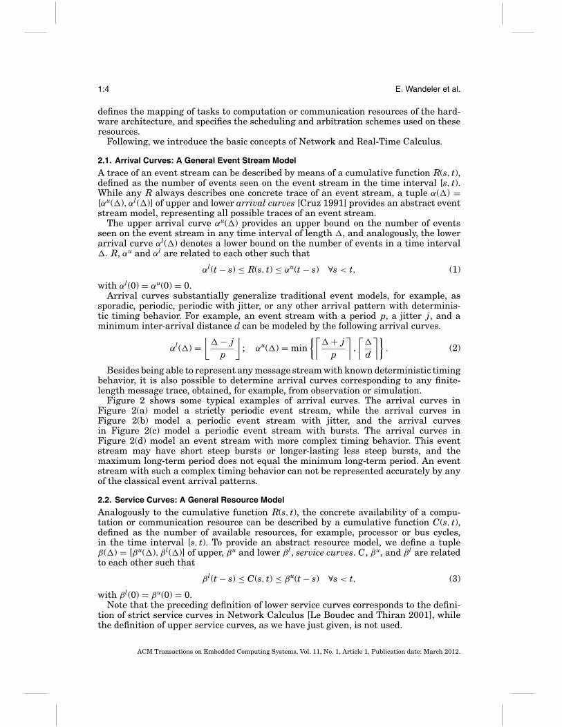
Fig. 7. Delay and backlog obtained from arrival and service curves.

When processed by a sequence of GP components, the total end-to-end delay experi-enced by an event is bounded by

dmax ≤ Del(αu, βl

1 ⊗ βl2 ⊗ · · · ⊗ βl

n

). (10)

On the other hand, the maximum buffer space bmax that is required to buffer anevent stream with arrival curve α in the input queue of a GP component on a resourcewith service curve β is bounded by

bmax ≤ supλ≥0

{αu(λ) − βl(λ)} def= Buf (αu, βl). (11)

When the buffers of consecutive components access the same shared memory, the totalbuffer space is bounded by

bmax ≤ Buf(αu, βl

1 ⊗ βl2 ⊗ · · · ⊗ βl

n

). (12)

In Figure 7, the relations between α, β, dmax, and bmax are depicted graphically. Fromthis figure, we see that dmax and bmax are bounded by the maximum horizontal andmaximum vertical distance between the upper arrival curve and the lower servicecurve, respectively. This corresponds to the intuition that dmax and bmax occur when themaximum load arrives at the time of minimum resource availability.

3. PERFORMANCE ANALYSIS OF GREEDY SHAPERS

From now on, we will consider one-sided cumulative functions only, that is, R(t) ≡R(0, t) and C(t) ≡ C(0, t). In other words, we suppose that event streams start at t = 0and we consider the positive time domain only.

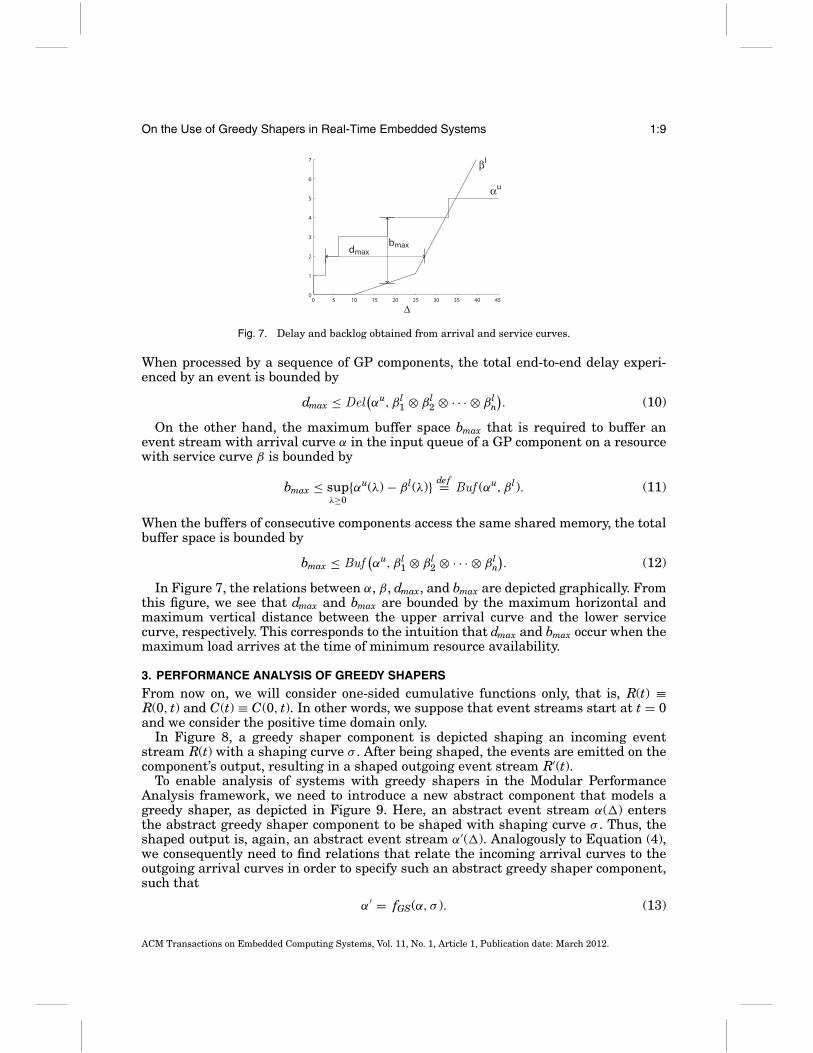
In Figure 8, a greedy shaper component is depicted shaping an incoming eventstream R(t) with a shaping curve σ . After being shaped, the events are emitted on thecomponent’s output, resulting in a shaped outgoing event stream R′(t).

To enable analysis of systems with greedy shapers in the Modular PerformanceAnalysis framework, we need to introduce a new abstract component that models agreedy shaper, as depicted in Figure 9. Here, an abstract event stream α(�) entersthe abstract greedy shaper component to be shaped with shaping curve σ . Thus, theshaped output is, again, an abstract event stream α′(�). Analogously to Equation (4),we consequently need to find relations that relate the incoming arrival curves to theoutgoing arrival curves in order to specify such an abstract greedy shaper component,such that

α′ = fGS(α, σ ). (13)



Fig. 8. A concrete greedy shaper that is shaping a concrete event stream.

Fig. 9. An abstract greedy shaper that is shaping an abstract event stream.

Following, we will first explain the behavior and implementation of concrete greedyshapers. We will then introduce the internal relations that define an abstract greedyshaper component.

3.1. Concrete Greedy Shapers

A greedy shaper with a shaping curve σ delays events of an input event stream suchthat the output event stream has σ as an upper arrival curve. Additionally, a greedyshaper ensures that no events get delayed any longer than necessary.

Greedy shapers can therefore be used to ensure that an event stream is upper-bounded by an upper arrival curve αu. For this, the event stream R is input to a greedyshaper with shaping curve σ ≤ αu. The output event stream R′ of the greedy shaper isthen upper-bounded by αu.

To analyze the behavior of a greedy shaper, consider a greedy shaper with shapingcurve σ which is subadditive and with σ (0) = 0. Assume that the shaper buffer isempty at time 0 and that it is large enough so that there is no event loss. The meaningof subadditivity, in this context and in relation to whether this property restricts theclass of shapers that can be analyzed, will be discussed in Section 3.3.

Le Boudec and Thiran [2001] prove that for an event trace R to input such a greedyshaper, the output event trace R′ can be computed as

R′ = R ⊗ σ. (14)

In practice, a greedy shaper with a shaping curve of

σ (�) =⌊

min∀i

{(bi) + ri�}⌋

(15)



ALGORITHM 1: Leaky bucket greedy shaper with bucket size b and filling rate r.Given:A clock c ∈ R≥0 that is continuously running and that can be reset to c = 0.

Initialize:reset clock c = 0;reset bucket fill level f = b;

while true doblocking read of event e from FIFO input buffer;f = min{ f + c · r, b};send event e;f = f − 1;reset c = 0;wait max{0,

1− fr };

end while

and with σ (0) = 0 can be implemented using a cascade of so-called leaky bucket greedyshapers. Every leaky bucket greedy shaper is a greedy shaper with a shaping curveof σi(�) = (bi) + ri�� and can be implemented using some sort of leaky bucket, withbucket size bi, that is filled (instead of emptied) at a constant rate of ri. If an eventarrives at such a leaky bucket greedy shaper, it can pass the shaper immediately if thefill level of the bucket is larger than or equal to 1. Otherwise, the event gets delayeduntil the bucket is filled enough. Finally, every event that is sent on the output of theshaper reduces the bucket fill level by 1.

At such a leaky bucket stage, the first bi� events of a burst can pass without anydelay. But further events of the burst will be delayed and can only pass at a rate ofri. If no events arrive for some time, the bucket will eventually be full again, allowinganother burst of bi� events to pass.

Algorithm 1 shows the pseudocode to implement a leaky bucket greedy shaper. Ini-tially, the bucket is full, and the clock is reset to c = 0. Then, the shaper does a blockingread on its first in, first out input buffer. If an event is available on the first in, firstout input buffer, it is immediately sent to the shaper output, but before sending theevent, the new bucket fill level f is computed as the sum of the last-computed bucketfill level and the amount c · r by which the bucket got filled since the last clock reset,and hence, the last update of the fill level. The fill level is thereby limited by the bucketsize b. Immediately after sending the event, the bucket fill level is reduced by 1, andthe clock is reset to c = 0. If necessary, the shaper then waits until the bucket fill levelis larger than or equal to 1 again before doing the next blocking read on its first in,first out input buffer.

Figure 10 depicts a shaping curve that can be implemented by a cascade of twoleaky buckets. The first leaky bucket has a bucket size of b1 = 1 and a leaking rate ofr1 = 1/4, while the second leaky bucket has a bucket size of b2 = 2.8 and a leaking rateof r2 = 1/15.

It is also possible to implement greedy shapers with more complex shaping curvesthan that of Equation (15). For this, the greedy shaper needs to consider the history ofsent events and compare it against the shaping curve to determine the next point intime when an event can pass the shaper. The implementation of such a greedy shapertypically would be more complex than a simple cascade of leaky bucket greedy shapers,and therefore, in practice, one would approximate a complex shaping curve with ashaping curve as defined in Equation (15).



0 10 20 30 40 50 60 70 800

1

2

3

4

5

6

7

8

9

10

σ

b1

b2

r2

r1

R’(t)R(t)

σb1, r1 b2, r2

Fig. 10. A greedy shaper that is implemented by a cascade of two leaky bucket stages and the resultingtotal shaping curve.

dmax,tot

dmax,GP

GPR’(t)

)t(’’R)t(R σ

Fig. 11. Cascade of a processing component and a greedy shaper that reshapes the output event stream.

In practice, one of the simplest examples of a shaper is the play-out buffer that isread at a constant rate. Play-out buffers are widely used in multimedia processing, andcan be implemented by a single leaky bucket greedy shaper.

3.2. Reshaping Comes For Free

An interesting property of greedy shapers is that reshaping does not increase delay orbuffer requirements. That is to say, if an event stream R(t) that is constrained by theupper arrival curve αu is the input to a processing component, as depicted in Figure 11,and if a greedy shaper with shaping curve σ ≥ αu is used to reshape the outputevent stream, then the maximum delay experienced by any event is not increased byadding the greedy shaper, that is, dmax, tot = dmax, GP. Moreover, if the greedy shaperwith shaping curve σ ≥ αu and the input buffer to the processing component access thesame shared memory, then the total buffer requirement is also not increased by addingthe greedy shaper, that is, bmax, tot = bmax, GP. These properties are sometimes referredto as “greedy shapers come for free” [Le Boudec and Thiran 2001].

3.3. Abstract Greedy Shapers

In order to embed greedy shapers into the Modular Performance Analysis framework,we need to determine the relation per Equation (13) that connects input and outputarrival curves. This way, we can analyze distributed embedded systems that containgreedy shapers as components and determine worst-case bounds on end-to-end delays,throughput, and buffer sizes. Therefore, the challenges posed in Thiele et al. [2000]and Schioler et al. [2005] concerning the possibility of modeling traffic shapers in theframework of Modular Performance Analysis (MPA) are solved.



THEOREM 3.1 (ABSTRACT GREEDY SHAPERS). Assume an event stream that is modeledas an abstract event stream with arrival curves [αu, αl] serves as input to a greedy shaperwith a subadditive shaping curve σ with σ (0) = 0. Then, the output of the greedy shaperis an event stream that can be modeled as an abstract event stream with arrival curves

αu′GS = αu ⊗ σ, (16)

αl′GS = αl ⊗ (σ�σ ). (17)

Further, the maximum delay and the maximum backlog at the greedy shaper arebounded by

dmax,GS = Del (αu, σ ), (18)bmax,GS = Buf (αu, σ ). (19)

PROOF. To prove Equation (16), we use the fact that R � R is the minimum upperarrival curve of a cumulative function R, and we use the properties

( f � g) � h = f � (g ⊗ h),( f ⊗ g) � g ≤ f ⊗ (g � g),

proven in Le Boudec and Thiran [2001]. We can then compute

R′ � R′ = (R ⊗ σ ) � (R ⊗ σ )= ((R ⊗ σ ) � R) � σ

= ((σ ⊗ R) � R) � σ

≤ (σ ⊗ (R � R)) � σ

≤ (σ ⊗ αu) � σ

= (αu ⊗ σ ) � σ

= αu ⊗ σ.

To prove Equation (17), we use the fact that R�R is the maximum lower arrivalcurve of a cumulative function R, and we use the property

( f ⊗ g)�(h ⊗ j) ≥ ( f �h) ⊗ (g� j),

which we prove in the Appendix. We can then compute

R′�R′ = (R ⊗ σ )�(R ⊗ σ )≥ (R�R) ⊗ (σ�σ )≥ αl ⊗ (σ�σ ).

To prove Equation (18), we compute

d(t) = inf{τ ≥ 0 : R(t) ≤ R′(t + τ )}= inf{τ ≥ 0 : 0 ≤ inf

0≤u≤t+τ{σ (t + τ − u) + R(u) − R(t)}}

≤ inf{τ ≥ 0 : 0 ≤ inf0≤u≤t

{σ (t − u + τ ) − αu(t − u)}}≤ inf{τ ≥ 0 : 0 ≤ inf

0≤v{σ (v + τ ) − αu(v)}}

= inf{τ ≥ 0 : sup0≤v

{αu(v) − σ (v + τ )} ≤ 0}

= sup0≤�

{inf{τ ≥ 0 : αu(�) ≤ σ (� + τ )}}.



To prove Equation (19), we compute

b(t) = R(t) − R′(t) = R(t) − (σ ⊗ R)(t)= R(t) − inf

0≤u≤t{σ (t − u) + R(u)}

= R(t) + sup0≤u≤t

{−σ (t − u) − R(u)}

= sup0≤u≤t

{R(t) − R(u) − σ (t − u)}

≤ sup0≤u≤t

{αu(t − u) − σ (t − u)}

= sup0≤v≤t

{αu(v) − σ (v)}

≤ sup0≤�

{αu(�) − σ (�)}.

Theorem 3.1 supposes that the shaping curve σ is subadditive. As defined in the Ap-pendix, we have σ (a)+σ (b) ≥ σ (a+b) for all a, b ≥ 0, in this case. In order to understandwhether this is a restriction, let us consider a time interval of length a + b. If σ is notsubadditive, then we could find some partition of this interval into two subintervalsof length a and b such that σ (a + b) > σ (a) + σ (b). Remember that σ (�) bounds thenumber of output events in any time interval of length �. Therefore, in any interval ofsize a + b, we can not have more events than σ (a) + σ (b). As a result of this discussion,we conclude that σ (a + b) can be lowered without changing the behavior of the shaper.In other words, the specification of the shaping curve σ was not tight, that is, it couldbe lowered without any change of the shaper behavior. This opens the question of howwe can determine a “tight” subadditive shaping curve from a given one which is notsubadditive. According to the Appendix, the tightest subadditive shaping curve is givenby the subadditive closure σ . If the given shaping curve σ is not subadditive, then itshould be replaced by σ before applying Theorem 3.1.

Equations (16) and (17) can now be used as internal relations of an abstract greedyshaper, and Equations (18) and (19) can be used to analyze delay guarantees and bufferrequirements of greedy shapers in a performance model.

4. APPLICATIONS AND CASE STUDIES

In this section, we analyze the two system designs depicted in Figure 1. The analysisresults will clearly reveal the positive influence of greedy shapers on a system’s perfor-mance and buffer requirements, when applied internally or on a system’s robustness,when applied externally. We deliberately chose two small system designs that clearlyfocus on the influence of the greedy shapers and does not dilute the analysis resultsby any possibly hard recognizable influences of other system properties. Modular Per-formance Analysis with Real-Time Calculus have already been used several times toanalyze bigger and more complex system designs [Chakraborty et al. 2003; Wandeleret al. 2006], and the abstract greedy shapers can seamlessly be integrated into biggerperformance models.

4.1. Internal Shaping for System Improvement

Consider a distributed real-time system with two CPU’s that communicate via a sharedbus, as depicted on the left side in Figure 1. C PU1 and C PU2 both process an incomingevent stream S1 and S2, respectively, and send the resulting event streams S′′

1 and S′′2

via the shared bus to other components. The shared bus implements a fixed-priorityprotocol in which sending the events from C PU1 has priority over sending the eventsfrom C PU2. Events that are ready to be sent get buffered in the communication network



interfaces CNI1 and CNI2 that connect C PU1 and C PU2, respectively, with the sharedbus.

In this system, S′′1 may differ considerably from S1. For example, S′′

1 may be burstyeven when S1 is a strictly periodic event stream. This may happen, for example, ifother tasks, besides TS1, are executed on C PU1 using a TDMA scheduling policy, orif FP scheduling is used and TS1 has a low priority. In both cases, the processor maynot be available to TS1 during some time interval in which all arriving events of S1 getbuffered, and it may be fully available to TS1 during a later time interval in which allthe buffered events will be processed and emitted, leading to a burst on S′′

1.Now, suppose that event stream S′′

1 is bursty. Whenever a burst of events arrives onS′′

1, the shared bus gets fully occupied until all buffered events of S′′1 are sent. During

this period, event stream S′′2 will receive no service, and S′′

2 will experience a delaycaused by the burstiness of S′′

1. Moreover, the buffer demand in CNI2 will increasewith the increasing burstiness of S′′

1.In this system, it may be an interesting option to place a greedy shaper at the output

of C PU1 that shapes event stream S′1. This greedy shaper will limit the burstiness of

S′′1, and will, therefore, reduce the influence of C PU1 and S1 to the delay of S′

2 and tothe buffer requirements of CNI2.

To investigate the effect of adding greedy shapers to the system with internal reshap-ing in Figure 1, we analyze it with Modular Performance Analysis, using the abstractgreedy shaper component that we introduced in Section 3.

We assume that S1 and S2 are both strictly periodic with a period p = 1ms. Further,we model both CPU’s as bounded delay resources. The CPU may not be available toprocess the tasks TSi for up to 5ms, but after this period of at most 5ms, the processoris fully available and can process five events per ms (βu

CPU1 = βuCPU2 = 5�[e/ms],

βlCPU1 = βl

CPU2 = max{0,� − 5}[e/ms]), and the bus can send 2.5 events per ms (βuBUS =

βlBUS = 2.5�[e/ms]).With this specification, we analyze the four different system designs that are depicted

in Figure 12. First, we analyze the system without greedy shapers (Figure 12(a));secondly, we place a greedy shaper only at the output of C PU1 to shape S′

1(Figure 12(b)); then, we place a greedy shaper only at the output of C PU2 to shapeS′

2 (Figure 12(c)); and finally, we add two greedy shapers to shape both S′1, as well as

S′2 (Figure 12(d)). We use the upper arrival curves αu

S1 and αuS2 as shaping curves σ1

and σ2, respectively, and we assume that the buffers of the greedy shapers and thecorresponding processing tasks access the same memory.

Using the four performance models, we analyzed the maximum required bufferspaces of the different buffers, as well as the end-to-end delays of both event streams S1and S2. The results, computed with the Real-Time Calculus (RTC) Toolbox for Matlab[Wandeler and Thiele], are shown in Table I.

From the results, we learn that placing greedy shapers helps to reduce the total bufferrequirements from 25 down to at most 14 events that need to be buffered. Moreover,the greedy buffers also reduce the end-to-end delay of both event streams, namely by7.4% for S1, and by a total of 40% for S2.

When we look at the results, we also recognize the well-known property of greedyshapers that reshaping is for free. Since we use σ1 = αu

S1 and σ2 = αuS2, the greedy

shapers effectively only reshape S11 and S2

2 , and therefore, the buffer requirements ofC PU1 and C PU2 are not affected by adding the greedy shapers.

4.2. Input Shaping for Separation of Concerns

Typical large embedded systems often process several event streams in parallel. Toachieve separation of concerns in such systems, they are often implemented using



CNI1

GP

βCPU1

α1’GS GP

α1’’ α1’’’α1

βBUS

σ1

(d)

CPU1

CNI2

GP

βCPU2

α2’GS GP

α2’’ α2’’’α2

σ2

CPU2

CNI1

GP

βCPU1

GPα1’’ α1’’’α1

βBUS

(c)

CPU1

CNI2

GP

βCPU2

α2’GS GP

α2’’ α2’’’α2

σ2

CPU2

CNI1

GP

βCPU1

α1’GS GP

α1’’ α1’’’α1

βBUS

σ1

(b)

CPU1

CNI2

GP

βCPU2

GPα2’’ α2’’’α2

CPU2

CNI1

GP

βCPU1

GPα1’’ α1’’’α1

βBUS

(a)

CPU1

CNI2

GP

βCPU2

GPα2’’ α2’’’α2

CPU2

Fig. 12. Performance models for four system architecture scenarios with internal reshaping.

Table I. Effect of ReShaping

Buffer DelayShapers C PU1 C PU2 CNI1 CNI2 T ot S1 S2

none 6 6 4 9 25 5.4 9S1 6 6 1 6 19 5 5.8�% — — −75% −33% −24% −7.4% −36%S2 6 6 4 4 20 5.4 8.6�% — — — −56% −20% — −4.4%both 6 6 1 1 14 5 5.4�% — — −75% −89% −44% −7.4% −40%

time-triggered scheduling policies, or servers. While these scheduling policies help todecouple the influence of the various event streams to each other, they often do not usethe available resources efficiently.

On the other hand, powerful methods were developed to analyze systems with event-triggered scheduling policies, such as RM or EDF. In these systems, resources are usedefficiently, but on the downside, the various event streams may heavily influence eachother. Slight changes in the timing behavior of a high-priority stream may increasethe total delay of a lower-priority stream considerably, possibly leading to a misseddeadline or to buffer overflows somewhere in the system.

To overcome this problem, greedy shapers may be placed at the input to such systems.Every incoming event stream Si gets shaped with an individual shaping curve σi that



α1 GS GPα1’ α1’’

βCPUσ1


σ2


σ3

α1 GPα1’’

βCPU

α2 GPα2’’

α3 GPα3’’

)b()a(

Fig. 13. Performance models with external input shaping.

Table II. Effect of Input Shaping

Without Shaping With Shapingd1 d2 d3 d1 d2 d3

j1 = 0 2.86 8.57 20 2.86 8.57 20j1 = 0.1 2.86 8.57 28.57 2.96 8.57 20

�% 0 0 +43% +3.5% 0 0

corresponds to its design-time timing specification. The system can then be analyzedusing the design-time timing specifications, and at runtime, non-adherence of Si to itstiming specification will have no influence on the delay of any other event streams butwill, at most, increase the total delay of Si itself. Moreover, no buffers will overflowinside the system. Instead, only the buffers of the greedy shapers themselves mayoverflow. But since these buffers are clearly localized at the boundary of the system,individual handling policies could easily be implemented.

Let’s assume a real-time system, as shown on the right side of Figure 1. Here, asingle CPU processes three event streams with a fixed-priority scheduling policy. Thehigh-priority stream S1 is strictly periodic with p1 = 5ms; the medium-priority streamS2 is strictly periodic with p2 = 10ms; and the low-priority stream S3 is strictly periodicwith p3 = 20ms. The CPU processes 0.35 events per ms.

To illustrate the influence of greedy shapers at the input of such a system, we adda jitter of j1 = 0.1ms to stream S1. We then analyze the effect of this to the end-to-end delays of the three event streams, both without (as in Figure 13(a)) and with (asin Figure 13(b)) greedy shapers. The results, computed using Modular PerformanceAnalysis, are shown in Table II.

Looking at the results, we clearly see the big influence of the little non-adherence ofS1 on the maximum delay of the completely independent stream S3, if no input shapingis applied. On the other hand, we observe that input shaping effectively isolates theinfluence of the malicious input stream S1 to the other present event streams. Now,only S1 is affected by its own malbehavior.

4.2.1. Input Shaping for NRT Event Streams in Real-Time Systems. Inspired by the applica-tion of greedy shapers for input shaping for separation of concerns, one could also usegreedy shapers to shape non-real-time event streams, as depicted in Figure 14. Here,the non-real-time event streams, are processed with the highest priority, guaranteeinga good reactivity and typically short delays, and the greedy shaper guarantees that



αNRT GS GPαNRT’ αNRT’’

βCPUσNRT

αRT, dRT GPαRT’’

(a) (b)

CPU1

TNRTRNRT’’RNRT σ1

TRTR2’’RRT, dRT

Fig. 14. System model (a) and performance model (b) with input shaping for NRTtraffic.

the load created by the non-real-time events is limited, such that the real-time eventstreams remain schedulable.

In such an application, the greedy shaper is an alternative to typical server imple-mentations, such as the periodic [Sha et al. 1986] or the deferrable server [Strosnideret al. 1995], and in a certain respect, the greedy shaper also behaves like a server. Theadvantage of the greedy shaper, however, is its flexibility through the parameterizableshaping curve σNRT. With an appropriate shaping curve, a shaper can, for example,guarantee a reactive periodic service, such as the deferrable server, but additionally,it may also allow a burst of service from time to time. Moreover, a greedy shaper istypically easy to implement.

The main question that then arises in an application, as depicted Figure 14, ishow to dimension the greedy shaper. How should σNRT be chosen such that the maxi-mum possible service to the non-real-time events is provided without jeopardizing theschedulability of the real-time event streams?

In Wandeler and Thiele [2005], the theory of Real-Time Interfaces was first intro-duced, providing methods for finding the maximum allowable shaping curve σNRT.With Real-Time Interfaces, the maximum allowable non-real-time input load α′

NRT tothe system in Figure 14 can be computed as

αuNRT, max = RT −α

(αu

RT(� − dRT), βlCPU

), (20)

with

RT −α(β ′, β)(�) = β(� + λ) − β ′(� + λ)for λ = sup{τ : β ′(� + τ ) = β ′(�)}, (21)

where αuRT models the maximum real-time input load, dRT denotes the relative deadline

of the real-time events, and βlCPU models the minimum available service from the CPU.

The greedy shaper must then only enforce that the load on its output is limited byαu

NRT, max, which is easily achieved by setting the shaping curve equal to this upperbound. Without any loss, the shaping curve can even be ensured to be subadditive bysetting it equal to the subadditive closure of the following upper bound (see Appendix).

σNRT = αuNRT, max. (22)

The methods presented in Wandeler and Thiele [2005] also allow for the computationof σNRT for systems with more than one real-time event stream and for even morecomplex systems with mixed and hierarchical scheduling.

As an example, consider a system similar to the one depicted in Figure 14 but withthree real-time event streams with decreasing priorities: RRT,1 has a period of 100ms,a jitter of 40ms, and an execution demand of 25ms; RRT,2 has a period of 200ms, a jitter



Fig. 15. Input shaping curve σNRT for the NRTtraffic in the example system.

of 150ms, and also an execution demand of 25ms; and RRT,3 has a period of 500ms andan execution demand of 100ms. The relative deadlines of all real-time event streamsequal their periods. To compute the shaping curve σNRT for the non-real-time eventstreams in this system, we use the methods presented in Wandeler and Thiele [2005]and Equation (22).

From the result depicted in Figure 15, we learn that within this system, any non-real-time event streams that are upper-bounded by σNRT will be served immediatelywith the highest priority, that is, they will not be delayed by the input shaper. This isthe case if the input arrival curve αu

NRT, max is completely within the grey shaded area.If there are events that contravene this upper bound, they will be delayed by the inputshaper to ensure schedulability of the real-time streams. This is the case if the inputarrival curve αu

NRT, max is tight and reaches the white area. The corresponding delay canbe computed using Equation (18).

5. CONCLUSIONS

We introduced a new method for analyzing greedy shapers and we embedded thismethod into the Modular Performance Analysis framework of Chakraborty et al. [2003]and Thiele et al. [2000], by introducing a new abstract component that models a greedyshaper. This approach enables system-level performance analysis of real-time systemswith greedy shapers. We proved the applicability of the presented methods throughperformance analysis of two case study systems with greedy shapers. In these casestudy systems, we analyzed the detailed buffer requirements of all system componentsand provided end-to-end delay guarantees for the processed event streams. The anal-ysis thereby clearly revealed the positive influence of greedy shapers on the system’sperformance and buffer requirements.

APPENDIX

Min-Max Algebra

The operators ⊗, �, and � are defined as

( f ⊗ g)(�) = inf0≤λ≤�

{ f (� − λ) + g(λ)}, (23)



( f � g)(�) = supλ≥0

{ f (� + λ) − g(λ)}, (24)

( f � g)(�) = infλ≥0

{ f (� + λ) − g(λ)}. (25)

A curve f is subadditive if

f (a) + f (b) ≥ f (a + b) ∀a, b ≥ 0. (26)

The subadditive closure f of a curve f is the largest subadditive curve with f ≤ fand is computed as

f = min{ f, ( f ⊗ f ), ( f ⊗ f ⊗ f ), . . .}. (27)

If f is interpreted as an arrival curve, then any trace R that is upper-bounded by f isalso upper-bounded by the subadditive closure f .

LEMMA 5.1. Given nonnegative, monotonic increasing functions f, g, h, j : R �→ R

with f (t) = g(t) = h(t) = j(t) = 0 for all t ≤ 0. Then

( f ⊗ g)� (h ⊗ j) ≥ ( f � h) ⊗ (g� j).

PROOF. We have, by definition of the operators,

( f ⊗ g)� (h ⊗ j) = infλ≥0

sup0≤b≤λ

inf0≤a≤�+λ

[ f (a) − h(b) + g(� + λ − a) − j(λ − b)].

We will consider three cases depending on the value of a.

—b ≤ a ≤ b + �:

infλ≥0

sup0≤b≤λ

infb≤a≤b+�

[ f (a) − h(b) + g(� + λ − a) − j(λ − b)]

= infλ≥0

sup0≤b≤λ

inf0≤a′≤�

[ f (a′ + b) − h(b) + g(� + λ − a′ − b) − j(λ − b)]

≥ infλ≥0

inf0≤b≤λ

inf0≤a′≤�

[ f (a′ + b) − h(b) + g(� + λ − a′) − j(λ)]

≥ infλ≥0

inf0≤b

inf0≤a′≤�

[ f (a′ + b) − h(b) + g(� + λ − a′) − j(λ)]

= inf0≤a′≤�

[inf0≤b

( f (a′ + b) − h(b)) + infλ≥0

(g(� + λ − a′) − j(λ))]

=( f � h) ⊗ (g� j).

Note that we used variable substitutions and the relation

supa

{u(a) + v(a) } ≥ u(a0) + infa

{v(a)}.



—b + � ≤ a ≤ � + λ:

infλ≥0

sup0≤b≤λ

infb+�≤a≤�+λ

[ f (a) − h(b) + g(� + λ − a) − j(λ − b)]

= infλ≥0

sup0≤b≤λ

inf0≤a′≤λ−b

[ f (a′ + b + �) − h(b) + g(λ − b − a′) − j(λ − b)]

= infλ≥0

sup0≤b′≤λ

inf0≤a′≤b′

[ f (a′ + � + λ − b′) − h(λ − b′) + g(b′ − a′) − j(b′)]

≥ infλ≥0

inf0≤b′≤λ

inf0≤a′≤b′

[ f (a′ + � + λ − b′) − h(λ − b′)]

≥ inf0≤b

inf0≤a′

[ f (a′ + � + b) − h(b)]

= inf0≤b

[ f (� + b) − h(b)]

= f � h.

—0 ≤ a ≤ b:

infλ≥0

sup0≤b≤λ

inf0≤a≤b

[ f (a) − h(b) + g(� + λ − a) − j(λ − b)]

= infλ≥0

sup0≤b≤λ

inf0≤a′≤b

[ f (b − a′) − h(b) + g(� + a′ + λ − b) − j(λ − b)]

≥ infλ≥0

inf0≤b′≤λ

inf0≤a′≤b

[g(� + a′ + λ − b) − j(λ − b)]

≥ inf0≤λ

inf0≤a′

[g(� + a′ + λ) − j(λ)]

= inf0≤λ

[g(� + λ) − j(λ)]

=g� j.

Now we have

( f ⊗ g)� (h ⊗ j) ≥ min{( f � h) ⊗ (g� j), f � h, g� j}= ( f � h) ⊗ (g� j).

REFERENCES

CHAKRABORTY, S., KUNZLI, S., AND THIELE, L. 2003. A general framework for analyzing system properties inplatform-based embedded system designs. In Proceedings of the 6th Design, Automation and Test inEurope (DATE). 190–195.

CHAKRABORTY, S., KUNZLI, S., THIELE, L., HERKERSDORF, A., AND SAGMEISTER, P. 2003. Performance evaluation ofnetwork processor architectures: Combining simulation with analytical estimation. Comput. Netw. 41, 5,641–665.

CRUZ, R. 1991. A calculus for network delay. IEEE Trans. Inform. Theory 37, 1, 114–141.GONZALEZ HARBOUR, M., GUTIERREZ GARCIA, J., PALENCIA GUTIERREZ, J., AND DRAKE MOYANO, J. 2001. MAST:

Modeling and analysis suite for real time applications. In Proceedings of the 13th Euromicro Conferenceon Real-Time Systems. IEEE Computer Society, 125–134.

GRINGERI, S., SHUAIB, K., EGOROV, R., LEWIS, A., KHASNABISH, B., AND BASCH, B. 1998. Traffic shaping, band-width allocation, and quality assessment for mpeg video distribution over broadband networks. IEEENetworks 12, 6, 94–107.

LE BOUDEC, J. AND THIRAN, P. 2001. Network Calculus—A Theory of Deterministic Queuing Systems for theInternet. Lecture Notes in Computer Science, vol. 2050, Springer-Verlag.

POP, P., ELES, P., AND PENG, Z. 2003. Schedulability analysis and optimization for the synthesis of multiclus-ter distributed embedded systems. In Proceedings of the 6th Design, Automation and Test in Europe(DATE’03). 184–189.



REXFORD, J., BONOMI, F., GREENBERG, A., AND WONG, A. 1997. Scalable architectures for integrated trafficshaping and link scheduling in high-speed ATM switches. IEEE J. Select. Areas Comm. 15, 5, 938–950.

RICHTER, K., JERSAK, M., AND ERNST, R. 2003. A formal approach to mpsoc performance verification. IEEEComput. 36, 4, 60–67.

SCHIOLER, H., JESSEN, J., NIELSEN, J. D., AND LARSEN, K. G. 2005. CyNC—towards a general tool for perfor-mance analysis of complex distributed real-time systems. In Proceedings of the WiP Session of the 17thEUROMICRO Conference on Real-Time Systems (ECRTS). IEEE, 61–64.

SHA, L., LEHOCZKY, J. P., AND RAJKUMAR, R. 1986. Solutions for some practical problems in prioritized preemptivescheduling. In Proceedings of the IEEE Real-Time Systems Symposium (RTSS). IEEE, 181–191.

SHIN, I. AND LEE, I. 2003. Periodic resource model for compositional real-time guarantees. In Proceedings ofthe IEEE Real-Time Systems Symposium (RTSS). IEEE, 2–13.

SHIN, I. AND LEE, I. 2004. Compositional real-time scheduling framework. In Proceedings of the IEEE Real-Time Systems Symposium (RTSS). IEEE, 57–67.

STROSNIDER, J. K., LEHOCZKY, J. P., AND SHA, L. 1995. The deferrable server algorithm for enhanced aperiodicresponsiveness in hard real-time environments. IEEE Trans. Comput. 44, 1, 73–91.

THIELE, L., CHAKRABORTY, S., AND NAEDELE, M. 2000. Real-time calculus for scheduling hard real-time systems.In Proceedings of the IEEE International Symposium on Circuits and Systems (ISCAS). Vol. 4. 101–104.

WANDELER, E., MAXIAGUINE, A., AND THIELE, L. 2006. Performance analysis of greedy shapers in real-timesystems. In Proceedings of the Design, Automation and Test in Europe (DATE). 444–449.

WANDELER, E. AND THIELE, L. Real-time calculus (RTC) toolbox.http://www.mpa.ethz.ch/Rtctoolbox.

WANDELER, E. AND THIELE, L. 2005. Real-time interfaces for interface-based design of real-time systems withfixed priority scheduling. In Proceedings of the 5th ACM Conference on Embedded Software (EMSOFT).80–89.

WANDELER, E. AND THIELE, L. 2006. Interface-based design of real-time systems with hierarchical scheduling.In Proceedings of the 12th IEEE Real-Time and Embedded Technology and Applications Symposium(RTAS). 243–252.

WANDELER, E., THIELE, L., VERHOEF, M., AND LIEVERSE, P. 2006. System architecture evaluation using modularperformance analysis—a case study. Softw. Tools Technol. Transfer 8, 6, 649–667.

Received January 2007; revised May 2007; accepted June 2007


1 on the use of greedy shapers in real-time … · shaper to conform again to the input trafﬁc...

Documents