1 on optimal quasi-orthogonal space-time block codes with

1

On Optimal Quasi-Orthogonal Space-Time

Block Codes with Minimum Decoding

ComplexityHaiquan Wang, Dong Wang, and Xiang-Gen Xia

Abstract

Orthogonal space-time block codes (OSTBC) from orthogonaldesigns have both advantages of

complex symbol-wise maximum-likelihood (ML) decoding andfull diversity. However, their symbol

rates are upper bounded by3/4 for more than2 antennas for complex symbols. To increase the symbol

rates, they have been generalized to quasi-orthogonal space-time block codes (QOSTBC) in the literature

but the diversity order is reduced by half and the complex symbol-wise ML decoding is significantly

increased to complex symbol pair-wise (pair of complex symbols) ML decoding. The QOSTBC has been

modified by rotating half of the complex symbols for achieving the full diversity while maintaining the

complex symbol pair-wise ML decoding. The optimal rotationangles for any signal constellation of any

finite symbols located on both square lattices and equal-literal triangular lattices have been found by

Su-Xia, where the optimality means the optimal diversity product (or product distance). QOSTBC has

also been modified by Yuen-Guan-Tjhung by rotating information symbols in another way such that it

has full diversity and in the meantime it has real symbol pair-wise ML decoding (the same complexity

as complex symbol-wise decoding) and the optimal rotation angle for square and rectangular QAM

constellations has been found.

In this paper, we systematically study general linear transformations of information symbols for

QOSTBC to have both full diversity and real symbol pair-wiseML decoding. We present the optimal

transformation matrices (among all possible linear transformations not necessarily symbol rotations) of

information symbols for QOSTBC with real symbol pair-wise ML decoding such that the optimal diversity

product is achieved for bothgeneralsquare QAM andgeneral rectangularQAM signal constellations.

Haiquan Wang is with College of Communications Engineering, Hangzhou Dianzi University, Hangzhou, China. Email:

[email protected]. Dong Wang is with Wireless Communications and Networking Department, Philips Research North

America, Briarcliff Manor, NY, 10510. Email:[email protected]. Xiang-Gen Xia is with the Department of

Electrical and Computer Engineering, University of Delaware, Newark, DE 19716. Email:[email protected]. Haiquan

Wang and Dong Wang were with the Department of Electrical andComputer Engineering, University of Delaware, Newark, DE

19716. This work was supported in part by the Air Force Office of Scientific Research (AFOSR) under Grant No. FA9550-08-

1-0219 and the National Science Foundation under Grant CCR-0325180.

October 30, 2008 DRAFT

2

Furthermore, our newly proposed optimal linear transformations for QOSTBC also work for general

QAM constellations in the sense that QOSTBC have full diversity with good diversity product property

and real symbol pair-wise ML decoding. Interestingly, the optimal diversity products for square QAM

constellations from the optimal linear transformations ofinformation symbols found in this paper coincide

with the ones presented by Yuen-Guan-Tjhung by using their optimal rotations. However, the optimal di-

versity products for (non-square) rectangular QAM constellations from the optimal linear transformations

of information symbols found in this paper are better than the ones presented by Yuen-Guan-Tjhung by

using their optimal rotations. In this paper, we also present the optimal transformations for the co-ordinate

interleaved orthogonal designs (CIOD) proposed by Khan-Rajan for rectangular QAM constellations.

Index Terms

Complex symbol-wise decoding, Hurwitz-Radon family, linear transformations of information sym-

bols, optimal product diversity, quasi-orthogonal space-time block codes, real symbol pair-wise decoding.

I. INTRODUCTION

Orthogonal space-time block codes (OSTBC) from orthogonaldesigns have attracted considerable

attention [3]–[20] since Alamouti code [3] was proposed. OSTBC have two advantages, namely they

have fast maximum-likelihood (ML) decoding, i.e., complexsymbol-wise decoding, and they have full

diversity. However, the symbol rates of OSTBC for more than two antennas are upper bounded by3/4

for most complex information symbol constellations no matter how large a time delay is or/and no matter

whether a linear processing is used [15]. To increase the symbol rates for complex symbols, OSTBC

have been generalized to quasi OSTBC (QOSTBC) in Jafarkhani[21], Tirkkonen-Boarin-Hottinen [22]

and Papadias-Foschini [23], [24], also in Mecklenbrauker-Rupp [25], [26] under the name “extended

Alamouti codes,” by relaxing the orthogonality between allcolumns of a matrix. The relaxation of the

orthogonality in QOSTBC increases the ML decoding complexity and in fact, the ML decoding of

QOSTBC is in general complex symbol pair-wise (two complex symbols as a pair) decoding. Moreover,

the original QOSTBC in [21], [22], [23], [24], [25], [26] do not have full diversity. For example, the

diversity order of QOSTBC for 4 antennas is only 2, which is half of the full diversity order 4. The idea

of rotating information symbols in a QOSTBC to achieve full diversity and maintain the complex symbol

pair-wise ML decoding has appeared independently in [28], [29], [30], [31]. Furthermore, the optimal

rotation anglesπ/4 andπ/6 of the above mentioned information symbols for any signal constellations

on square lattices and equal-literal triangular lattices,respectively, have been obtained in Su-Xia [30] in


3

the sense that the diversity products are maximized. In thisapproach, half of the complex information

symbols are rotated. It has been shown in [30] that the QOSTBCwith the optimal rotations of the complex

symbols have achieved the maximal diversity products amongall possible linear transformations of all

complex symbols. A different rotation method for QOSTBC hasbeen proposed in Yuen-Guan-Tjhung

[37], [38], [39] such that the QOSTBC has full diversity and its ML decoding becomes real symbol

pair-wise decoding that has the same complexity as the complex symbol-wise decoding. Furthermore,

the optimal rotation angle has been found to bearctan(1/2)/2 = 13.29 in [37], [38], [39] when the

signal constellations are square or rectangular QAM. What is gained with this type of rotations is that the

complex symbol pair-wise ML decoding is reduced to the real symbol pair-wise ML decoding and what

is sacrificed is that the optimal diversity product obtainedin [30] from the complex symbol rotations is

reduced but the diversity product reduction is not significant. As a remark, for rectangular QAM signal

constellations and OSTBC, the complex symbol-wise ML decoding can be reduced to real symbol-wise

decoding that reaches the minimum decoding complexity. ForQOSTBC, it is not hard to show that the

real symbol pair-wise decoding has already reached the minimum decoding complexity and it can not

be reduced to real symbol-wise decoding due to the non-existence of rate1 complex orthogonal designs

[14] as we shall see later.

A different method from the QOSTBC to increase symbol rates in OSTBC has been proposed in

Khan-Rajan [32]–[36] by placing OSTBC on diagonal and jointly selecting information symbols across

all the OSTBC on the diagonal. This scheme is called co-ordinate interleaved orthogonal design (CIOD

or CID) in [32]–[36], where it was shown that CIOD can also achieve full diversity and have the real

symbol pair-wise ML decoding similar to QOSTBC. All the results are only for square QAM signal

constellations.

In this paper, we systematically study general linear transformations (not only limited to rotations)

of information symbols (their real and imaginary parts are separately treated) for QOSTBC to have

both full diversity and real symbol pair-wise ML decoding. We first present necessary and sufficient

conditions on a general linear transformation of symbols for QOSTBC such that it has a real symbol

pair-wise ML decoding. We then present the optimal transformation matrices (among all possible linear

transformations that are not necessarily rotations or orthogonal transforms) of information symbols for

QOSTBC with real symbol pair-wise ML decoding such that the optimal diversity products are achieved.

The optimal transformation matrices are obtained for bothgeneralsquare QAM andgeneral rectangular

QAM signal constellations. By applying the optimal linear transformations for rectangular QAM signal

constellations to any QAM signal constellations, we find that the QOSTBC also have full diversity,


4

good diversity products, and the real symbol pair-wise ML decoding. Interestingly, the optimal diversity

products for square QAM signal constellations from the optimal linear transformations of information

symbols found in this paper coincide with the ones presentedin [37], [38], [39], which means that the

optimal rotation of two real parts and two imaginary parts obtained in [37], [38], [39] already achieves the

optimal diversity products. However, the optimal diversity products for (non-square) rectangular QAM

signal constellations from the optimal linear transformations of information symbols found in this paper

are better than the ones with the optimal rotations presented in [37], [38], [39]. Also note that, since a

general linear transformation does not require the orthogonality, our study covers signal constellations

on not only square lattices but also other lattices as we discuss in Section III-D.

In this paper, we also present the optimal linear transformations of symbols and the optimal diversity

products for CIOD studied in [32]–[36] for general rectangular QAM signal constellations that can

be treated as a generalization of the results for square QAM signal constellations presented in [32]–

[36]. We compare QOSTBC using optimal symbol linear transformations with CIOD also using optimal

symbol linear transformations. It turns out that these two schemes perform the same in terms of both the

ML decoding complexity and the diversity product, but the peak-to-average power ratio (PAPR) of the

QOSTBC is better than that of the CIOD as what has also been pointed out in [37], [39].

This paper is organized as follows. In Section II, we describe the problem of interest in more details.

In Section III-A, we present necessary and sufficient conditions on general linear transformations for

QOSTBC to have real symbol pair-wise ML decoding. In Sections III-B, III-C, and III-E, we present

the optimal linear transformations for QOSTBC for both general square and rectangular QAM signal

constellations and the optimal linear transformations of symbols for CIOD for rectangular QAM signal

constellations, respectively. In Section III-D, we investigate optimal linear transformations for arbitrary

QAM constellations on general lattices. In Section IV, we set up a more general problem in terms of

generalized Hurwitz-Radon families for QOSTBC with fast MLdecoding. In Section V, we present some

numerical simulation results. Most of the proofs are in Appendix.

Some Notations: Z, R, C denote the sets of all integers, all real numbers, and all complex numbers,

respectively. Capital English letters, such asA, B, C, denote matrices and small case English letters,

such asr, s, p, q, denote scalars unless otherwise specified.Im denotes the identity matrix of sizem×m.

A†, At andA∗ denote the conjugate transpose, transpose, and conjugate of matrix A, respectively. tr(A)

denotes the trace of matrixA.


5

II. M OTIVATION AND PROBLEM DESCRIPTION

In this section, we describe the problem in more details. Consider a quasi-static and flat Rayleigh

fading channel withn transmit andm receive antennas:

Y =

√

ρ

nCH + W, (1)

whereC ∈ C is a transmitted signal matrix, i.e., a space-time codewordmatrix, of sizeT × n, T is

the time delay,C is a space-time code,H is the channel coefficient matrix of sizen × m, andY , W

are received signal matrix and AWGN noise matrix, respectively, of sizeT × m, andρ is the SNR at

each receiver. Assume that the entrieshij of H are independent, zero-mean complex Gaussian random

variables of variance1/2 per dimension and they are constant in each block of sizeT . Also assume

that the entrieswij of W are independent, zero-mean Gaussian random variables of variances1/2 per

dimension. Assume at the receiver, channelH is known. Then, the ML decoding is

arg minC∈C

‖Y −√

ρ

nCH‖2

F , (2)

where ‖ · ‖F denotes the Frobenious norm. Based on the pair-wise symbol error probability analysis

for the above ML decoding, the following rank and diversity product criteria were proposed in [1], [2]

for the design of a space-time codeC: The minimum rank of difference matrixC − C over all pairs

of distinct codeword matricesC and C is as large as possible; The minimum of the product of all the

nonzero eigenvalues of matrix(C − C)†(C − C) over all pairs of distinct codeword matricesC and C

is as large as possible.

Clearly, when a space-time codeC has full diversity (or full rank), i.e., any difference matrix of any

two distinct codeword matrices inC has full rank, the product of all the nonzero eigenvalues of matrix

(C− C)†(C− C) in the diversity product criterion is the same as the determinantdet((C− C)†(C− C)).

Since, in this paper we are only interested in full diversityspace-time codes, in what follows we use the

following diversity product definition as commonly used in the literature:

ζ∆=

1

2√

Tmin

C 6=C∈C|det((C − C)†(C − C))| 1

2n , (3)

and it is desired that the diversity product of a space-time code is maximized for a given size, which in

fact covers the full rank criterion since ifC−C is not full rank then the determinantdet((C−C)†(C−C))

is always0.

Notice that a space-time codeword matrixC hasT rows andn columns and the full rankness forces

that T ≥ n for a fixed numbern of transmit antennas. This means that, forR bits/channel use (orR


6

bits/s/Hz), the size of a space-time codeC has to be at least2Rn for n transmit antennas while it is

only 2R in single antenna systems. Thus, in general the complexity of the ML decoding in (2) increases

exponentially in terms ofn, the number of transmit antennas, if there is no structure onC is used.

Orthogonal space-time block codes (OSTBC) from orthogonaldesigns first studied in [3], [4] do have

simplified ML decoding as we can briefly review below.

A. Orthogonal Space-Time Block Codes

A complex orthogonal design(COD) in complex variablesz1, z2, · · · , zk is aT×n matrixG(z1, · · · , zk)

such that

(i) any entry ofG(z1, · · · , zk) is a complex linear combination ofz1, z2, · · · , zk, z∗1 , z∗2 , · · · , z∗k.

(ii) G satisfies the orthogonality

(G(z1, · · · , zk))†G(z1, · · · , zk) = (|z1|2 + |z2|2 + · · · + |zk|2)In (4)

for all complex valuesz1, z2, · · · , zk.

From a CODG(z1, · · · , zk), an OSTBC can be formed by using it and restricting all the complex variables

zi in finite signal constellationsSi: C = G(z1, · · · , zk) : zi ∈ Si, 1 ≤ i ≤ k. With the orthogonality

(ii) and the linearity (i), the ML decoding (2) can be simplified as follows:

minC∈C

‖Y −√

ρ

nCH‖2

F

= minC∈C

tr(Y †Y ) −√

ρ

ntr(Y †CH + H†C†Y ) +

ρ

ntr(H†C†CH)

(5)

= minz1,··· ,zk

‖Y −√

ρ

nG(z1, · · · , zk)H‖2

F

= minz1,··· ,zk

tr(Y †Y ) −√

ρ

ntr(Y †G(z1, · · · , zk)H + H†(G(z1, · · · , zk))†Y )

+ρ

ntr(H†(G(z1, · · · , zk))

†G(z1, · · · , zk)H)

= minz1,··· ,zk

tr(Y †Y ) −√

ρ

ntr(Y †G(z1, · · · , zk)H + H†(G(z1, · · · , zk))†Y )

+ρ

ntr(H†H)(|z1|2 + · · · + |zk|2))

(6)

= minz1∈S1

f1(z1) + minz2∈S2

f2(z2) + · · · + minzk∈Sk

fk(zk), (7)

wherefi(zi) is a quadratic form of the only complex variablezi. From (7), one can see that the original

k-tuple complex symbol ML decoding

minz1,··· ,zk

‖Y −√

ρ

nG(z1, · · · , zk)H‖2

F = min(z1,··· ,zk)∈S1×···×Sk

‖Y −√

ρ

nG(z1, · · · , zk)H‖2

F


7

is reduced tok independent complex symbol-wise decodings:minzi∈Sifi(zi) for 1 ≤ i ≤ k. For

convenience, we call the decoding in (7)complex symbol-wise decoding. What we want to emphasize

here is that in the above complexity reduction, the finite complex signal constellationsSi can be any

sets of finite complex numbers and do not have to be rectangular or square such as 16-QAM. With the

properties (i)-(ii) in a COD, it is easy to check thatC has full diversity.

When signal constellationsSi are not arbitrary but have rectangular shapes, the above complex symbol-

wise decoding can be further reduced as follows. Letj =√−1. A signal constellationS is called

rectangular QAM denoted as RQAM if

S =

z | z =n1d

2+ j

n2d

2: ni ∈ Ni for i = 1, 2

, (8)

where

Ni∆= −(2Ni − 1),−(2Ni − 3), · · · ,−1, 1, · · · , 2Ni − 3, 2Ni − 1, (9)

whereN1 and N2 are two positive integers andd is a real positive constant that is used to adjust the

total signal energy. For convenience, we assume allk signal constellationsSi for information symbols

zi are the same,S. WhenS is an RQAM, by noting|zi|2 = d2

4 n2i1 + d2

4 n2i2, (7) becomes

minC∈C

‖Y −√

ρ

nCH‖2

F

= minn11∈N1

f11(n11) + minn12∈N2

f12(n12) + minn21∈N1

f21(n21) + minn22∈N2

f22(n22)

+ · · · + minnk1∈N1

fk1(nk1) + minnk2∈N2

fk2(nk2) (10)

wherefi1 andfi2 are independent quadratic forms of integer variablesni1 andni2, respectively. If each

complex variablezi in (7) is treated as a pair of real numbers, the complex symbol-wise decoding in

(7) has the same complexity of the real symbol pair-wise decoding, i.e., two real symbols are searched

jointly. From (10), one can see that if the signal constellation S is an RQAM, the complex symbol-wise

(or real symbol pair-wise) decoding (7) can be reduced to thereal symbol-wise decoding in (10) that

has the minimal decoding complexity. Unfortunately, the symbol ratesk/T for an OSTBC or COD are

upper bounded by3/4 for more than two transmit antennas, i.e.,n > 2, and for most complex signal

constellations no matter how large a time delayT is [15].

B. Quasi Orthogonal Space-Time Block Codes

In order to increase the symbol rates of OSTBC, quasi orthogonal space-time block codes (QOSTBC)

from quasi orthogonal designs have been proposed by Jafarkhani [21], Tirkkonen-Boarin-Hottinen [22],


8

Papadias-Foschini [23], [24], and also Mecklenbrauker-Rupp [25], [26]. For4 transmit antennas, letA

andB be two Alamouti codes, i.e.,

A =

z1 z2

−z∗2 z∗1

, B =

z3 z4

−z∗4 z∗3

.

Then, the QOSTBC by Jafarkhani [21] and by Tirkkonen-Boarin-Hottinen [22] are

CJ =

A B

−B∗ A∗

andCTBH =

A B

B A

,

respectively. Similar constructions were also presented in [24], [25], [27]. Although their forms are

different, their performances are identical. One can see that the symbol rates in both schemes are1.

However, their rank is only2 that is only half of the full rank4. Furthermore, due to the first two

columns and the last two columns are not orthogonal each other, the complex symbol-wise decoding (7)

does not hold in general. However, since the first two columnsare orthogonal and the last two columns

are also orthogonal, the original4-tuple ML decoding can be reduced into the following complexsymbol

pair-wise decoding

minCJ∈CJ

‖Y −√

ρ

nCJH‖2

F = minz1,z4

g14(z1, z4) + minz2,z3

g23(z2, z3)

minCT BH∈CT BH

‖Y −√

ρ

nCTBHH‖2

F = minz1,z3

g13(z1, z3) + minz2,z4

g24(z2, z4),

wheregij is a quadratic form of complex variableszi andzj . As mentioned before, although the symbol

rates are increased from3/4 to 1 in the above QOSTBC, their diversity order is only2. To have full

diversity for QOSTBC, the idea of rotating symbolsz3 and z4 in CJ and rotating symbolsz3 and z4

in CTBH have been independently proposed in [28], [29], [30], [31].Furthermore, the optimal rotation

angles for arbitrary signal constellations located on bothsquare lattices and equal-literal triangular lattices

have been obtained in [30] such that the optimal possible diversity products for the QOSTBC are achieved.

SinceCJ and CTBH have the same performance, for convenience, in what followswe only consider

CTBH , i.e., the QOSTBC appeared in [22] as follows.

Let Gn(z1, · · · , zk) be aT × n complex orthogonal design in complex variablesz1, · · · , zk (for its

designs, see for example [11], [12], [13]). LetA = Gn(z1, · · · , zk) and B = Gn(zk+1, · · · , z2k). We

consider the following quasi orthogonal design (QCOD)Q2n(z1, · · · , z2k):

Q2n(z1, · · · , z2k) =

A B

B A

. (11)


9

Then,

Q†2nQ2n =

aIn bIn

bIn aIn

. (12)

where

a =

2k∑

i=1

|zi|2 and b =

k∑

i=1

(ziz∗k+i + zk+iz

∗i ). (13)

From this equation and (5), the ML decoding becomes

minC∈C

‖Y −√

ρ

nCH‖2

F = minz1,zk+1

g1(z1, zk+1) + · · · + minzk,z2k

gk(zk, z2k). (14)

wheregi is a quadratic form ofzi and zk+i, which is calledcomplex symbol pair-wise decoding. By

rotating zk+i aszk+i ∈ Sk+i = ejθs : s ∈ Si from zi, it is shown in [28], [29], [30], [31], QOSTBC

with rotated symbols can achieve full diversity. Sincezi andzk+i are jointly decoded anyway, the symbol

rotation does not change the complex symbol-wise decoding.

One can see that the above complex symbol pair-wise decodingholds for QOSTBC for any signal

constellationszi ∈ Si. Similar to OSTBC studied before, when signal constellations Si are RQAM in

(8), it can be further reduced as follows.

When symbolsz1, · · · , z2k are all taken from RQAM, i.e.,zi can be written aszi = ri + jsi, where

ri andsi are independent real numbers. Then,

a =

2k∑

i=1

(|ri|2 + |si|2), b =

k∑

i=1

2(rirk+i + sisk+i) (15)

and the ML decoding (14) becomes

minC∈C

‖Y −√

ρ

nCH‖2

F

= minr1, rk+1

f11(r1, rk+1) + mins1, sk+1

f12(s1, sk+1) + minr2, rk+2

f21(r2, rk+2)

+ mins2, sk+2

f22(s1, sk+1) + · · · + minrk, r2k

fk1(rk, r2k) + minsk, s2k

fk2(sk, s2k), (16)

wherefij, i = 1, 2, · · · , k, j = 1, 2, are independent of each other and also quadratic forms of independent

variablesri, rk+i whenj = 1 and of independent variablessi, sk+i whenj = 2. The decoding in (16) is

real symbol pair-wise decodingthat has the same complexity as complex symbol-wise decoding in (7).

Note that the decomposition (16) is due to the form of QOSTBC and its properties (11)-(15), and the

independence of all the real and imaginary parts of all information symbols. As we mentioned earlier,

QOSTBC (11) has only diversity order2, i.e., half of the full diversity4. The questionnow is whether

we can rotate the information symbols in such a way that the QOSTBC has full diversity and in the

meantime, a real symbol pair-wise ML decoding similar to (16) also holds. This problem has been studied


10

by Yuen-Guan-Tjhung [37], [38], [39] and in [38], they proposed to rotate(ri, rk+i) into (pi, pk+i) and

(si, sk+i) into (qi, qk+i), while in [37], [39], they proposed to rotate(ri, si) into (pi, qi) and(rk+1, sk+i)

into (pk+i, qk+i), which is similar to the idea of rotating complex symbols in (14). This type of rotations

has been proposed earlier in co-ordinate interleaved orthogonal designs (CIOD or CID) by Khan-Rajan

in [32]–[36], which is a different approach than QOSTBC and shall be compared in more details later.

Furthermore, the optimal rotation angle for square QAM and rectangular QAM signal constellations in

QOSTBC have been obtained in [37], [38], [39].

C. General Symbol Transformation Formulation

One can see that the reason why the ML decoding of a QOSTBC can be reduced to the real symbol

pair-wise decoding in (16) is due to properties (12) and (15). From (15), one can see that a real symbol

pair-wise ML decoding exists as long as the quadratic formulas a and b in (15) of four real symbols

pi, pk+i, qi, qk+i can be decomposed into sums of two independent forms each of which has two real

variables and the two forms have disjoint variables, respectively. This motivates the following general

linear transformation formulation of symbols such that a real symbol pair-wise ML decoding of QOSTBC

is maintained.

For convenience, all information symbol constellationsSi are assumed the same,S, that is a finite set

of at least four points on the integer/square lattice

Z[j] = z = n1 + jn2 : n1, n2 ∈ Z. (17)

We assume thatS is not equivalent to any PAM constellation, i.e., not all points in S are collinear (on

a single straight line). Then, the detailedencodingis as follows and shown in Fig. 1:

• A binary information sequence is mapped to pointszi in S aszi = ri + jsi for 1 ≤ i ≤ 2k.

• For eachi, 1 ≤ i ≤ k, take a pre-designed real linear transformUi and the real vector(ri, si, rk+i, sk+i)t

of dimension4 is transformed to another real vector(pi, qi, pk+i, qk+i)t of dimension4:

(pi, qi, pk+i, qk+i)t = Ui(ri, si, rk+i, sk+i)

t, (18)

whereUi is non-singular.

• Form complex variablesxi = pi + jqi for 1 ≤ i ≤ 2k.

• With these complex variablesxi, form a QOSTBCQ2n(x1, x2, · · · , x2k) that is used as a space-time

block code and transmitted through2n transmit antennas.


11

zi = ri + jsi

zk+i = rk+i + jsk+i

xi = pi + jqi

xk+i = pk+i + jqk+i

Q2n(x1, · · · , x2k)Ui

- - - -

Binary Information

symbol

mapping

Linear Quasi-orthogonal

space-time codeTransmit

transformsequences

Fig. 1. Encoding of an QOSTBC.

The question now is how to design a real linear transformations Ui of size 4 × 4 for a QOSTBC to

possess a real symbol pair-wise ML decoding and to have full diversity (or optimal diversity product).

In order to study a real symbol pair-wise ML decoding, let us study a andb in (15). Let

gi(pi, qi, pk+i, qk+i)∆= p2

i + q2i + p2

k+i + q2k+i, (19)

fi(pi, qi, pk+i, qk+i)∆= 2(pipk+i + qiqk+i). (20)

To possess a real symbol pair-wise ML decoding, linear transformationUi in (18) needs to be chosen

such that one of the following three cases holds

Case 1. Functionsgi andfi can be separated as

gi(pi, qi, pk+i, qk+i) = gi1(ri, si) + gi2(rk+i, sk+i),

fi(pi, qi, pk+i, qk+i) = fi1(ri, si) + fi2(rk+i, sk+i).


gi(pi, qi, pk+i, qk+i) = gi1(ri, rk+i) + gi2(si, sk+i),

fi(pi, qi, pk+i, qk+i) = fi1(ri, rk+i) + fi2(si, sk+i).


gi(pi, qi, pk+i, qk+i) = gi1(ri, sk+i) + gi2(si, rk+i),

fi(pi, qi, pk+i, qk+i) = fi1(ri, sk+i) + fi2(si, rk+i).

With the above encoding and properties, the ML decoding can be similarly described below. For the

illustration purpose, assume Case 1 holds for a design ofUi. Then, the ML decoding becomes

min(z1,··· ,z2k)∈S2k

‖Y −√

ρ

nQ2n(x1, · · · , x2k)H‖2

F

= minr1, s1

v1(r1, s1) + minr2, s2

v2(r2, s2) + · · · + minr2k, s2k

v2k(r2k, s2k), (21)


12

where we notice thatzi = ri + jsi. Real symbol pair-wise ML decodings for other two cases can be

similarly derived.

For Case 1, theith real and imaginary parts of theith complex symbolzi are decoded jointly, i.e., it

is the same as the complex symbolzi symbol-wise decoding. Since its real and imaginary parts are not

separated in the decoding, the signal constellationsSi for zi can be any constellations.

For Case 2, the real parts of theith and the(k+ i)th complex symbolszi andzk+i are decoded jointly

and the imaginary parts of theith and the(k + i)th complex symbolszi and zk+i are decoded jointly.

In this case, real parts and imaginary parts of complex symbols are required to be independent. Thus,

signal constellationsSi andSk+i for zi andzk+i have to be square or rectangular QAM.

For Case 3, the real part of theith complex symbolzi and the imaginary part of the(k + i)th complex

symbol zk+i are decoded jointly and the imaginary part of theith symbolzi and the real part of the

(k + i)th complex symbolzk+i are decoded jointly. In this case, similar to Case 2, signal constellations

Si andSk+i for zi andzk+i have to be square or rectangular QAM too.

It is not hard to see that in terms of real symbol pair-wise decoding, the above three cases are the only

possibilities. One might want to ask why a transformationUi is only used for four variables in (18) but

not for more variables. The answer to this question is rathersimple and it is because of the particular

forms of the quadratic formsa and b in (15) and (13) that appear in the ML decoding of a QOSTBC

due to the structure of a QOSTBC (12). To include more than 4 variables does not do anything better in

terms of real symbol pair-wise ML decoding and diversity product.

The main goal of the remaining of this paper is to investigatehow to design a linear transformations

Ui in (18) such that the above encoded QOSTBCQ2n(x1, · · · , x2k) has a real symbol pair-wise ML

decoding in terms of real information symbolsri andsi for 1 ≤ i ≤ 2k in each of the above three cases,

and full diversity and furthermore the diversity product ismaximized.

III. D ESIGNS OFL INEAR TRANSFORMATION MATRICES Ui

In this section, we first characterize all linear transformation matricesUi in (18) for Cases 1-3, i.e.,

for QOSTBC to possess a real symbol pair-wise ML decoding. Wethen present the optimalUi in the

sense that the diversity products of the QOSTBC are maximized.


13

A. Necessary and Sufficient Conditions onUi for Real Symbol Pair-Wise ML Decoding

First of all, the two quadratic forms ofpi andqi andpk+i andqk+i in (19)-(20) can be formulated as

gi(pi, qi, pk+i, qk+i) = p2i + q2

i + p2i+1 + q2

i+1 = (pi, qi, pk+i, qk+i)

I2 0

0 I2

pi

qi

pk+i

qk+i

, (22)

fi(pi, qi, pk+i, qk+i) = 2(pipk+i + qiqk+i) = (pi, qi, pk+i, qk+i)

0 I2

I2 0

pi

qi

pk+i

qk+i

. (23)

In terms of the information symbolsri, si, rk+i, sk+i through linear transformations (18), these quadratic

forms can be further expressed as

gi(ri, si, rk+i, sk+i)∆= gi(pi, qi, pk+i, qk+i) = (ri, si, rk+i, sk+i)U

ti

I2 0

0 I2

Ui

ri

si

rk+i

sk+i

, (24)

fi(ri, si, rk+i, sk+i)∆= fi(pi, qi, pk+i, qk+i) = (ri, si, rk+i, sk+i)U

ti

0 I2

I2 0

Ui

ri

si

rk+i

sk+i

. (25)

Theorem 1. Let Ui be a4× 4 non-singular matrix with all real entries used in (18). Then, we have the

following results.

(i) Case 1 holds if and only ifUi can be written as

Ui =

Ui1 Ui2

Ui1Ri1 Ui2Ri2

, (26)

whereUi1, Ui2, Ri1, Ri2 are 2 × 2 matrices of real entries,R2i1 = I2 and R2

i2 = I2, and

Rti1U

ti1Ui2 + U t

i1Ui2Ri2 = 0. (27)

(ii) Case 2 holds if and only ifUi can be written as

Ui =

Ui1 Ui2

Ui1Ri1 Ui2Ri2

P1, (28)


14

whereUi1, Ui2, Ri1, Ri2 are the same as in (i) for Case 1 and

P1 =

1 0 0 0

0 0 1 0

0 1 0 0

0 0 0 1

.

(iii) Case 3 holds if and only ifUi can be written as

Ui =

Ui1 Ui2

Ui1Ri1 Ui2Ri2

P2, (29)

whereUi1, Ui2, Ri1, Ri2 are the same as in (i) for Case 1 and

P2 =

1 0 0 0

0 0 0 1

0 0 1 0

0 1 0 0

.

Its proof is in Appendix. From what was discussed in Section II-C, if Ui in (18) satisfies Theorem

1, then the QOSTBC has a real symbol pair-wise ML decoding. Although this is the case, as what was

explained in Section II-C, different cases may require information signal constellationsSi differently.

If Ui satisfies (i) in Theorem 1, then information signal constellationsSi can be any QAM and not

necessarily square or rectangular QAM. On the other hand, ifUi satisfies (ii) or (iii) in Theorem 1, then

information signal constellationsSi have to be square or rectangular QAM for a real symbol pair-wise

ML decoding. WhenUi satisfies (i) in Theorem 1, the quadratic objective functions gi(ri, si, rk+i, sk+i)

and fi(ri, si, rk+i, sk+i) in (24) and (25) can be re-written as follows:

gi(ri, si, rk+i, sk+i) = (ri, si)(Uti1Ui1 + Rt

i1Uti1Ui1Ri1)

ri

si

+(rk+i, sk+i)(Uti2Ui2 + Rt

i2Uti2Ui2Ri2)

rk+i

sk+i

, (30)

fi(ri, si, rk+i, sk+i) = (ri, si)(Rti1U

ti1Ui1 + U t

i1Ui1Ri1)

ri

si

+(rk+i, sk+i)(Rti2U

ti2Ui2 + U t

i2Ui2Ri2)

rk+i

sk+i

. (31)


15

In what follows, we only consider linear transformationsUi that satisfy Theorem 1. From Theorem

1, one can see that there may be infinitely many options of suchlinear transformationsUi satisfying

Theorem 1, i.e., there are infinitely many options ofUi in (18) such that the QOSTBC has a real symbol

pair-wise ML decoding. The question now is whichUi is optimal in the sense thatUi satisfies Theorem

1 and the diversity product of the QOSTBC is maximized when the mean transmission signal power

is fixed. In what follows, we present solutions forUi of the following optimal linear transformation

problem:

maxUi satisfies Theorem 1

ζ(Q2n(x1, · · · , x2k)), (32)

when the mean transmission signal power is fixed, whereQ2n is a QOSTBC,ζ(Q2n(x1, · · · , x2k)) is

the diversity product of QOSTBCQ2n as defined in (3), andxi are defined in the encoding in Section

II-C as shown in Fig. 1.

Before we come to the solution of (32), let us see the rotations proposed in [38], [37], [39]. In [38],

only rotations for(ri, rk+i) and (si, sk+i) are used:

(pi, pk+i)t = R(ri, rk+i)

t and (qi, qk+i)t = R(si, sk+i)

t (33)

whereR is a 2 × 2 rotation. This rotation only corresponds to Case 2 and the correspondingUi in (18)

in terms of the form in (ii) in Theorem 1 for the rotation in (33) can be written as

Ui1 =

cos(γ) sin(γ)

0 0

, Ui2 =

0 0

cos(γ) sin(γ)

, Ri1 = Ri2 =

0 1

−1 0

. (34)

In [37], [39], rotations are done individually for each complex symbol as follows:

(pi, qi)t = R(ri, si)

t and (pk+i, qk+i)t = R(rk+i, sk+i)

t (35)

whereR is a 2 × 2 rotation. This rotation corresponds to Case 1 and the correspondingUi in (18) in

terms of the form in (i) in Theorem 1 for the rotation in (35) can be written as

Ui1 =

cos(γ) sin(γ)

0 0

, Ui2 =

0 0

cos(γ) sin(γ)

, Ri1 =

0 −1

1 0

, Ri2 =

0 1

−1 0

.

(36)

It has been found in [37], [38], [39] that the optimal rotation angleγoptimal =12 arctan(1

2) in the sense

that the diversity product of the QOSTBC is maximized among all different rotation anglesγ for square

and rectangular QAM constellations.

Another remark we want to make here is that the optimal diversity product achieved by the optimal

complex symbol rotations for a QOSTBC in Su-Xia [30] has beenshown in [30] optimal among all


16

possible linear transformationsUi without any restriction. We may expect that the optimal diversity

product of a QOSTBC with the optimal solution ofUi in (32) for the real symbol pair-wise ML decoding

may be smaller than the optimal one obtained in [30] with the complex symbol pair-wise ML decoding

as we shall see in Section III-C.

B. Optimal Linear TransformationsUi for Square QAM

In this subsection, we consider square QAM, i.e.,M2-QAM for anyM . We present a solution of linear

transformationsUi for the optimization problem (32), which turns out to be independent of the sizeM2

of theM2-QAM constellations and is different from other QAM constellations, such as rectangular QAM

as we shall see in later subsections.

From a QOSTBC form (11) and the designs of complex orthogonalspace-time block codes [11], [12],

[13], one can see that in most COD designs, the complex symbols±xi or their complex conjugates±x∗i

or zeros are directly placed in an CODGn(x1, · · · , xk), i.e., no linear processing of these symbols is

used, therefore±xi or ±x∗i , or 0 are directly transmitted. Thus, the mean transmission signal power is

determined by the mean power of complex symbolsxi. Even for a CODGn(x1, · · · , xk) with linear

processing of symbols±xi or ±x∗i , as long as the QOSTBC patternQ2n is fixed, the mean transmission

signal power is also determined by the mean power of complex symbols xi. From the encoding in

Section II-C, the signal powers ofxi = pi + jqi are determined byUi in (18) and the information

symbolszi = ri + jsi whereri andsi are integers. SinceUi are not necessarily orthogonal transforms,

the problem of the mean signal power ofxi can be formulated as the real lattice packing problem [53]

as follows. The4k dimensional lattice ofpi and qi, i = 1, 2, ..., 2k, for the transmission signal can be

formulated in terms of the4k information integer lattice ofri andsi, i = 1, 2, ..., 2k:

p1

q1

pk+1

qk+1

...

pk

qk

p2k

q2k

=

U1 · · · 0...

. .....

0 · · · · · · Uk

r1

s1

rk+1

sk+1

...

rk

sk

r2k

s2k

(37)


17

whereri, si, i = 1, 2, · · · , 2k, are from the integer setZ and Ui are 4 × 4 non-singular real matrices.

Then, the mean signal power of the transmission signal latticepi, qi is reciprocal to the packing density of

the 4k dimensional real lattice, which is determined by the determinant of the lattice generating matrix:

1∏k

i=1 |det(Ui)|.

Therefore, the normalized diversity product of the QOSTBCQ2n in (11) in terms of the mean signal

power becomes:

ζ(Q2n)∆=

ζ(Q2n)(

∏ki=1 |det(Ui)|

)1/(4k), (38)

whereζ(Q2n) is the diversity product (3) of QOSTBCQ2n(x1, · · · , x2k). Thus, the optimization problem

(32) becomes: to find a non-singular linear transformationUi that satisfies Theorem 1 such that the above

normalized diversity productζ(Q2n) is maximized. For this optimization problem, we have the following

solution.

Theorem 2. Let

α = arctan(2) and R =

cos(α) sin(α)

sin(α) − cos(α)

, (39)

and P1 and P2 be the4 × 4 matrices defined in (ii) and (iii) in Theorem 1, respectively. For the three

cases in Section II-C, we have the following results, respectively.

(i) For Case 1, let

Ui =1√2

I2 I2

R −R

. (40)

Then, the above orthogonal matricesUi satisfy (i) for Case 1 in Theorem 1, i.e., the quadratic forms

fi in (19) andgi in (20) of 4 variables can be separated as Case 1, and furthermore,Ui are optimal

in the sense that the normalized diversity productζ(Q2n) in (38) is maximized among all other

non-singular linear transformationsUi that satisfy (i) in Theorem 1 and

maxUi in (i) Theorem 1

ζ(Q2n) =1

2√

2T(4

5)1/4. (41)

(ii) For Case 2, let

Ui =1√2

I2 I2

R −R

P1. (42)

Then, the above orthogonal matricesUi satisfy (ii) for Case 2 in Theorem 1 and they are optimal,

and the same maximum normalized diversity product in (41) isachieved.


18

(iii) For Case 3, let

Ui =1√2

I2 I2

R −R

P2. (43)

Then, the above orthogonal matricesUi satisfy (iii) for Case 3 in Theorem 1 and they are optimal,

and the same maximum normalized diversity product in (41) isachieved.

Its proof is in Appendix. As one can see, in this subsection, instead of using the actual mean

transmission signal power ofxi, we use the packing density in4k dimensional real lattices in the study.

As we shall see in the next subsection, the results in Theorem2 are indeed true for any finite size

square QAM, when the actual mean transmission signal power is used. In other words, when the actual

mean transmission power is fixed, the maximal diversity products are achieved by the optimal linear

transformations presented in Theorem 2. This is due to the square size of a square QAM that can be

well represented by a4k dimensional real lattice. The optimality result is also independent of the size

of a square QAM signal constellation.

Interestingly, although the optimal linear transformations Ui found in (ii) for Case 2 in Theorem 2 are

not the same as the optimal rotations (34) obtained in [38], the optimal diversity products for a QOSTBC

with the two different optimal transformations are the samefor squareQAM signal constellations as we

shall see later in the next subsection. The same conclusion can be drawn for the optimal rotations (36)

obtained in [37], [39] and the optimal linear transformations Ui found in (i) for Case 1. The optimal

rotation can be similarly obtained for (iii) for Case 3. Thismeans that in square QAM case, considering

the rotations as in (33)–(36) is sufficient in the sense that aQOSTBC has a real symbol pair-wise ML

decoding and in the meantime, the diversity product is maximized among all linear transformationsUi

that satisfy the conditions in Theorem 1. Note that since rotations in (33) are only for the real parts of

the ith and(k+ i)th complex symbols, and the imaginary parts of theith and(k+ i)th complex symbols,

separately, the rotations in (33) do not apply to Case 1 and Case 3.

It should be emphasized here that Case 1 is of particular interest. It is because the real symbol pair-wise

decoding is not for two real or two imaginary parts but for thereal and the imaginary parts of a single

complex information symbolzi. In this case, the signal constellationSi of zi can be any QAM. When

we consider (i) for Case 1 for an arbitrary QAM, although we are not able to prove that the aboveUi is

optimal, the obtained QOSTBC still has full diversity with good diversity product property. The details

about this issue shall be discussed in Section III-D later.

For rectangular QAM constellations, the situation is different and we use a different approach and find


19

that the optimal linear transformationsUi depends on the sizes/shapes of rectangular QAM constellations

as we shall see in the next subsection.

C. Optimal Linear TransformationsUi for Rectangular QAM (RQAM)

In this subsection, we consider RQAM signal constellationsin (8)-(9) with total N1N2 points. It is

not hard to see that the total energyE of the RQAM constellation in (8)-(9) is

E =2

3N1N2(2N

21 + 2N2

2 − 1)d2. (44)

For convenience, we assume the total energy of an RQAM constellation is normalized to1, i.e., E = 1.

Therefore, the distanced between two nearest neighboring points in the constellation becomes

d =

√

3

2N1N2(2N21 + 2N2

2 − 1). (45)

Since there exist2k variables in a QOSTBCQ2n(z1, · · · , z2k), the total energy of all these information

complex symbolsz1, · · · , z2k is 2k.

Let us consider Case 1 and the other two cases can be similarlydone. Linear transformationsUi in

(18) transform an information signal constellation RQAM for information symbolszi = ri + jsi and

zk+i = rk+i + jsk+i into another one for transmitted symbolsxi = pi + jqi andxk+i = pk+i + jqk+i,

1 ≤ i ≤ k, in Q2n(x1, · · · , x2k). For convenience, we require that the total energies of these two signal

constellations (before and after transformationsUi) are the same, i.e.,Ui, 1 ≤ i ≤ k, are total-energy-

invariant. The total-energy-invariance implies

k∑

i=1

∑

pi+jqi∈Di

(p2i + q2

i ) +∑

pk+i+jqk+i∈Dk+i

(p2k+i + q2

k+i)

= 2k, (46)

where, fori = 1, 2, · · · , 2k,

Di∆= pi + jqi : zi = ri + jsi ∈ RQAM, z(k+i)mod2k = r(k+i)mod2k + js(k+i)mod2k ∈ RQAM.

SinceUi satisfy (i) in Theorem 1, from (30),

p2i + q2

i + p2k+i + q2

k+i

= (ri, si)(Uti1Ui1 + Rt

i1Uti1Ui1Ri1)

ri

si

+ (rk+i, sk+i)(Uti2Ui2 + Rt

i2Uti2Ui2Ri2)

rk+i

sk+i

.


20

Thus, the total-energy-invariance (46) becomes

2k =

k∑

i=1

∑

ri+jsi∈RQAM(ri, si)(U

ti1Ui1 + Rt

i1Uti1Ui1Ri1)

ri

si

+

k∑

i=1

∑

rk+i+jsk+i∈RQAM(rk+i, sk+i)(U

ti2Ui2 + Rt

i2Uti2Ui2Ri2)

rk+i

sk+i

. (47)

Under the above energy invariance/normalization requirement, we have the following results.

Theorem 3. Regarding to Cases 1-3, we have the following results.

(i) For Case 1 and an RQAM in (8)-(9) with total energy1, i.e., (45). Letε1 = 4N21−1

2(2N21 +2N2

2−1) , ε2 =

4N22−1

2(2N21 +2N2

2−1) , α = arctan(2), ρ =√

512(1+ε1ε2)

, and

R1 =

cos(α) sin(α)

sin(α) − cos(α)

, P =

0 1

1 0

, Σ =

1 + ε1 1 − 2ε1

1 − 2ε1 2 − ε1

. (48)

Denote a diagonalization of symmetric matrixΣ as Σ = V tDV , whereD = diag(λ1, λ2), λ1, λ2

are the eigenvalues ofΣ and V is an orthogonal matrix. Let

Ui1 = ρV t

√λ1 0

0√

λ2

V ; Ui2 = ρV t

√λ2 0

0√

λ1

V P ; R2 = −PR1P. (49)

Then,

Ui =

Ui1 Ui2

Ui1R1 Ui2R2

i = 1, 2, · · · , k, (50)

satisfy (i) for Case 1 in Theorem 1, and are optimal in the sense that the diversity product of the

QOSTBC is maximized among allUi under (i) in Theorem 1 and the optimal diversity product is

ζoptimal,WWX =1

2√

2T

d

(1 + ε1ε2)1/4

=1

2√

2T

√

3

N1N2

√

16N41 + 16N4

2 + 48N21 N2

2 − 20N21 − 20N2

2 + 5. (51)

(ii) For Case 2,UiP1 with P1 in Theorem 1 is optimal, whereUi is defined in (50).

(iii) For Case 3,UiP2 with P2 in Theorem 1 is optimal, whereUi is defined in (50).

Its proof is in Appendix. A QOSTBCQ2n(x1, · · · , x2k) from a T × n COD Gn(x1, · · · , xk) has size

2T × 2n and thus in the optimal diversity product formula in (51), there is2T instead ofT as in the

diversity product definition (3). Note that the optimal diversity products in Theorem 3 are not in terms

of the normalized diversity products as used in the previoussubsection for square QAM constellations.


21

Since an RQAM covers a square QAM, i.e.,N1 = N2 = N in (8)-(9). In this case,ε1 = ε2 = 1/2 and

ρ =√

13 , Σ = 3

2I2. Thus,λ1 = λ2 = 32 andUi1 = Ui2 = 1√

2I2. Therefore, the optimalUi in Theorem 3

coincides with the one obtained in Theorem 2. Thus, we have following corollary.

Corollary 1. For a square QAM of sizeN2, the optimal diversity product of a QOSTBC among all

different linear transformationsUi in (18) that satisfy Theorem 1 is

ζoptimal,WWX =1

2√

2T

√

3√5N2(4N2 − 1)

. (52)

As mentioned in Section II-B that although the linear transformationUi for Case 1 and Case 2 in

Theorems 2 and 3 are different from the optimal rotations in (36) obtained in [37], [39] and the optimal

rotations in (34) obtained in [38], respectively, the corresponding optimal diversity products are the same,

i.e., (52), for a square QAM signal constellation of sizeN2.

From Theorem 2 and Theorem 3, one can see that, although we usetwo different energy normalization

methods and different proofs, the optimal linear transformations Ui are the same for square QAM

constellations. In this regard, Theorem 3 covers Theorem 2.

From Theorem 3, one can see that the optimal linear transformationsUi in Theorem 3 depend on the

size and the shape of an RQAM, i.e.,N1 andN2, which is not what a rotation in (34) and a rotation in

(36) can achieve. In fact, with the optimal rotation in (36) obtained in [37], [39] and the optimal rotation

in (34) obtained in [38], the optimal diversity product for an RQAM in (8)-(9) is

ζoptimal,YGT=1

2√

2T

(

4

5

)1/4

d =1

2√

2T

√

3√5N1N2(2N

21 + 2N2

2 − 1). (53)

It is not hard to see that

ζoptimal,WWX =1

2√

2T

(

1

1 + ε1ε2

)1/4

d ≥ 1

2√

2T

(

4

5

)1/4

d = ζoptimal,YGT, (54)

where the equality “=” holds if and only ifε1 = ε2 = 1/2, i.e.,N1 = N2 or square QAM. This concludes

the following result.

Theorem 4. The diversity product of a QOSTBC with the optimal linear transformationUi in Theorem

3 is greater than the one with the optimal rotation in (34) forany non-square RQAM.

Comparing with the optimal diversity productζoptimal,SX in [30] of a QOSTBC among all possible

linear transformations without any restriction in Theorem1 for RQAM, we have

ζoptimal,SX=1

2√

2Tdmin =

1

2√

2Td >

1

2√

2T

(

1

1 + ε1ε2

)1/4

d = ζoptimal,WWX, (55)


22

wheredmin is the minimum Euclidean distance of the signal constellation S and in the above RQAM

case,dmin = d. Note that in [30], it was shown that 12√

2Tdmin is an upper bound for the diversity product

of QOSTBC for any kind of linear transformations of information symbols and any signal constellation

and furthermore the one from the optimal rotation of the halfcomplex information symbols reaches the

upper bound.

As an example, for32(8 × 4)-RQAM, i.e., N1 = 4 andN2 = 2, and a4 × 4 QOSTBC, i.e.,T = 2,

we have

ζoptimal,SX=1

4(43264)1/4> ζoptimal,WWX =

1

4(49984)1/4>

1

4(54080)1/4= ζoptimal,YGT.

D. Linear TransformationsUi for Arbitrary QAM on Any Lattice

In this subsection, we first present the optimal linear transformationsUi for a rectangular QAM on an

arbitrary lattice and then investigate them for an arbitrary QAM on an arbitrary lattice.

As we explained before, when two real parts or two imaginary parts of two complex information

symbols, such asri, rk+i or si, sk+i, or one real part of one complex symbol and one imaginary

part of another complex symbol, such asri of zi andsk+i of zk+i, are jointly decoded but independently

among the pairs,the real and the imaginary parts of a complex number have to beindependent each

other. This requirement forces that a signal constellation that acomplex symbol belongs to has to be

RQAM on a square lattice. Thus, some commonly used signal constellations, such as the 32-QAM shown

in Fig. 2(a), and also equal-literal triangular lattices are excluded for the fast decoding. Therefore, Case

2 and Case 3 in Section II-C do not apply to an arbitrary QAM (non-rectangular QAM), such as the ones

in Fig. 2, that may have better energy compactness than RQAM,or other lattices than a square lattice.

On the other hand, if the real part and the imaginary part of a complex symbol are not separated into two

independent decodings, such as in Case 1, then the real part and the imaginary part of a complex symbol

do not have to be independentfor a real symbol pair-wise decoding for QOSTBC. In this case, a signal

constellation can be any set of finite complex numbers. For QOSTBC with a real symbol pair-wise ML

decoding, Case 1 is the only case for linear transformationsUi.

We first consider a rectangular QAM on any lattice (not necessarily square/integer) in the complex

plane. Any two real-dimensional lattice on the complex plane can be generated from the square integer

lattice through a2 × 2 non-singular real matrixΛ:

(r, s)t = Λ(r, s)t, (56)


23

t t t t

t t t t t t

t t t t t t

t t t t t t

t t t t t t

t t t t

-

6

(a) 32-QAM

t t t

t t t

t t

-

6

(b) 8-QAM

Fig. 2. Non-rectangular QAM.

where r and s are integers and it is simply called latticeΛ. A rectangular shape (or for simplicity

QAM) constellationS on latticeΛ corresponds to an RQAMS = (r, s)t : (r, s)t = Λ(r, s)t ∈ S on

a square/integer lattice. With this relationship, one might think that what we have obtained previously

could be applied to any rectangular QAM on any latticeΛ by absorbing the matrixΛ into the linear

transformationUi asUidiag(Λ−1,Λ−1) and then converting the problem to an RQAM on a square/integer

lattice. This is correct and incorrect. For a rectangular QAM S on a general latticeΛ, the real and the

imaginary partsr and s with z = r + js ∈ S may not be independent. Thus, the results for Case 2 or

Case 3 obtained previously do not apply to a rectangular QAM on an arbitrary lattice. Since in Case

1, the independence of the real and the imaginary parts of a complex symbol is not necessary, all the

results for Case 1 apply to an rectangular QAM on any latticeΛ for a non-singular generating matrixΛ.

This gives us the following corollary.

Corollary 2. For a rectangular QAMS on lattice Λ with a non-singular2 × 2 real matrix Λ, let

Ui = Uidiag(Λ−1,Λ−1) whereUi is defined in (i) for Case 1 in Theorem 3. Let information symbols

zi = ri + jsi be randomly taken inS and then follow the encoding procedure in Section II-C by replacing

ri, si, zi, pi, qi, xi, andUi with ri, si, zi, pi, qi, xi, and Ui, respectively. Then,Ui is optimal in the sense

that the QOSTBC has a real symbol pair-wise ML decoding and the diversity product is maximized.

For an arbitrary QAM on an arbitrary lattice we have the following result.

Theorem 5. Let Ui be defined in Corollary 2 andUi be the linear transformation defined in (i) in


24

Theorem 3. Then, the QOSTBC with this linear transformationhas full diversity and the real symbol

pair-wise ML decoding (21) for any QAM signal constellationon any lattice.

Proof. From the discussion of Corollary 2, without loss of generality, we only need to consider a

square lattice, i.e.,Λ = I2. In this case, letS be an arbitrary set of finite points on the square lattice.

Then, by adding proper points to it, constellationS can be made up into a RQAMS1 of sizeN1 ×N2.

Clearly, if a QOSTBC has full diversity for a larger constellationS1, it also has full diversity for a smaller

constellationS. For RQAM S1, we apply the result in (i) for Case 1 in Theorem 3 and know thatthe

QOSTBC has the optimal diversity product expressed in (51) that is not zero. This proves Theorem 5.

q.e.d.

Although we are not able to prove the optimality ofUi in Theorem 5 in terms of the optimal diversity,

we have the following conjecture.

Conjecture 1. For an arbitrary QAM S on an arbitrary lattice, there exists a tightestN1 × N2 RQAM

S1 in the sense that the Euclidean distance betweenS and S1 is minimized. With this RQAMS1, let Ui

be defined in Corollary 2. We conjecture thatUi is optimal in the sense that the QOSTBC reaches the

optimal diversity product.

Although we are not able to prove the optimality ofUi in (i) in Theorem 3 for an arbitrary QAM on

a square lattice, we can calculate the diversity product of the QOSTBC when thisUi is used:

ζWWX =1

2√

2T

(

1

1 + ε1ε2

)1/4

d, (57)

whereε1 andε2 are defined in Theorem 3,N1 andN2 are defined in Conjecture 1 andd is the Euclidean

distance of the two nearest neighboring points in constellation S with normalized total energy1. When

N1 = N2, i.e.,S is approximated by a tightest square QAM, the diversity product of the QOSTBC with

the aboveUi is

ζWWX =1

2√

2T

(

4

5

)1/4

d, (58)

whered is as before. The optimal diversity of the QOSTBC among all possible linear transformations is

[30]

ζoptimal,SX=1

2√

2Td, (59)

whered is the same as before, which can be achieved by optimally rotating half of the complex symbols

[30].


25

As an example, let us consider32-QAM in Fig. 2(a). By using the transformUi in (i) in Theorem

3, the diversity productζWWX = 0.0187 while the optimal diversity product in [30] isζoptimal,SX=

0.0198. Note that for the32(8 × 4)-RQAM, by using the optimal transformUi in (i) in Theorem 3,

the diversity productζoptimal,WWX = 1/(4(49984)1/4) = 0.0167 while the optimal diversity in [30] is

ζoptimal,SX= 1/(4(43264)1/4) = 0.0173 as calculated at the end of Section III-C.

E. Optimal Transformations for Co-ordinate Interleaved Orthogonal Designs (CIOD) for RQAM and

Some Comparisons

To increase the symbol rates of COD, a different approach hasbeen proposed by Khan-Rajan [32]–

[36], where they propose to place a COD on diagonal repeatedly with different information symbols and

then these different information symbols are interleaved in such a way that the final overall design has

full diversity, which is called aco-ordinate interleaved orthogonal design(CIOD). Its definition is given

below.

Let Gn(x1, · · · , xk) be aT ×n COD with complex variablesx1, · · · , xk as before. Forxi = pi + jqi,

1 ≤ i ≤ 2k, definexi = pi + jq(k+i)mod2k, 1 ≤ i ≤ 2k, as interleaved variables ofxi. A (2k, 2T, 2n)

CIOD Q2n(x1, · · · , x2k) is a 2T × 2n matrix and defined by

Q2n(x1, · · · , x2k) =

G(x1, · · · , xk) 0T×n

0T×n G(xk+1, · · · , x2k)

. (60)

By rotating a signal constellation properly, it has been shown in [32]–[36] that the above CIOD can

achieve full diversity. The encoding is similar to QOSTBC shown in Fig. 1. LetS be a signal constellation

of finite complex numbers. The encoding for a CIOD scheme is asfollows:

• Map a binary information sequence into symbolszi = ri + jsi in S, 1 ≤ i ≤ 2k.

• Rotate the mapped complex symbolszi = ri + jsi into xi = pi + jqi:

(pi, qi)t =

cos θ sin θ

− sin θ cos θ

(ri, si)t. (61)

• Define xi = pi + jq(k+i)mod2k, 1 ≤ i ≤ 2k.

• Transmit CIOD matrixQ2n(x1, · · · , x2k).

With this scheme, it has been shown in [32]–[36] that the CIODpossesses a real symbol pair-wise

ML decoding where(ri, si) are jointly decoded but independently in terms of indexi. Therefore, it is

similar to Case 1 in our study in Section II-C. Thus, for the real symbol pair-wise ML decoding, the

original signal constellationS does not have to be square or rectangular QAM. Also, the rotation in (61)


26

is not necessary and any2 × 2 real linear transformU does not change the real symbol pair-wise ML

decoding property. Regarding to diversity product property, the following result was obtained in [35].

Proposition 1. Let S be a square QAM on a square lattice, i.e., an RQAM in (8)-(9) with N1 = N2.

Then,θ = arctan(2)/2 is the optimal rotation angle in terms of the optimal diversity product for the

rotation (61) and the optimal diversity product with this optimal rotation angle is

ζoptimal,KRL=1

2√

2T

(

4

5

)1/4

d, (62)

whered is as before.

From the above result, one can see that the optimal diversityproducts in both QOSTBC and CIOD for

square QAMconstellations on square lattices are the same when a real symbol pair-wise ML decoding

is imposed:

ζoptimal,KRL = ζoptimal,YGT= ζoptimal,WWX.

For a non-square RQAM constellation, the optimal rotationshave not appeared so far. We next present

an optimality result for a non-square RQAM constellation.

Theorem 6. Let information signal constellationS be an RQAM defined in (8)-(9), andε1, ε2 be defined

as in Theorem 3. Defineα = arctan( 1√ε1ε2

), θ1 = arctan(√

5−12

√

ε2

ε1), θ2 = α − θ1, and

U =

cos(θ1)√2ε1

sin(θ1)√2ε2

− sin(θ2)√2ε1

cos(θ2)√2ε2

.

Replace the rotation in (61) by the above transformU . Then, the above transformationU is optimal

for a CIOD in terms of optimal diversity product among all non-singular linear transformations and the

optimal diversity product with this transformation is

ζoptimal,WWX,CIOD=1

2√

2T

(

1

1 + ε1ε2

)1/4

d, (63)

whered is the same as before.

Its proof is in Appendix. From this result and Theorem 3, one can see that the optimal diversity

products for QOSTBC and CIOD for any RQAM on a square lattice are the same, i.e.,

ζoptimal,WWX,CIOD= ζoptimal,WWX.

Thus, QOSTBC and CIOD with optimal linear transformations of complex symbols perform identically in

terms of both decoding complexity and diversity product property, which shall be verified via numerical


27

simulations in terms of symbol error rates vs. SNR for 4-QAM in Section V. However, since half of the

entries are0 in a CIOD, for a fixed mean transmission signal power, PAPR forQOSTBC is better than

that for CIOD as pointed out in [37], [39].

As a remark, the optimal linear transformationU in Theorem 6 is a rotation, i.e., orthogonal, if and

only if N1 = N2, i.e., the RQAM is square. Then, in this case,ε1 = ε2 = 1/2, α = arctan(2)

and θ1 = θ2 = α/2, and therefore it coincides with the optimal rotation in Proposition 1 obtained by

Khan-Rajan-Lee [35] and the optimal transformation becomes

U =

cos(α/2) sin(α/2)

− sin(α/2) cos(α/2)

.

IV. GENERAL SETTING WITH GENERALIZED HURWITZ-RADON FAMILIES

In this section, we discuss some generalizations of QOSTBC and CIOD we have previously studied.

It is not hard to see that, by splitting real and imaginary parts of complex symbols, both QOSTBC and

CIOD of k complex variables1 can be represented by a general linear dispersive form [45],[46] of 2k

real variables:

C(s1, s2, · · · , s2k) = s1A1 + s2A2 + · · · + s2kA2k, (64)

whereAi are T × n constant matrices of complex entries andsi are real variables. For convenience,

we assume information signal constellations are all RQAM. Then, all the real and imaginary parts are

independent when an i.i.d. information sequence is mapped to complex symbols in the RQAMs. LetSi

be the signal constellation for theith variablesi for 1 ≤ i ≤ 2k. Then, it is not hard to see that using

the aboveC as a space-time codeword matrix, it has a real symbolκ-tuple ML decoding (regardless of

a permutation of symbols) if and only if

(C(s1, · · · , s2k))†C(s1, · · · , s2k) = f1(s1, · · · , sκ)B1 + · · · + fτ (s2k−κ+1, · · · , s2k)Bτ , (65)

where τ = 2k/κ, Bi, 1 ≤ i ≤ τ , are n × n constant matrices, andfi, 1 ≤ i ≤ τ , are independent

functions of constant coefficients. If (65) holds for all real values of variablessi, whenκ = 1, it is not

hard to see that (65) is equivalent to

A†iAj + A†

jAi = 0 for 1 ≤ i 6= j ≤ 2k, (66)

1For convenience, we considerk complex variables instead of2k complex variables as previously used.


28

which is equivalent to thatS(s1, · · · , s2k) is a kind2 of COD (when it has full diversity that impliesA†iAi

has full rank) as also mentioned in [32]–[36] and [37], [38],[39]. This also implies that it is impossible

for QOSTBC or CIOD to have full diversity and real symbol-wise ML decoding unless its size is2× 2

by applying the COD symbol rate upper bound for a Hurwitz family in [15]. In other words, real symbol

pair-wise decoding is the lowest complexity decoding of a QOSTBC or CIOD can have, i.e., it is already

the minimum complexity decoding for QOSTBC or CIOD, for morethan2 transmit antennas.

For a generalκ, it is related to a generalized Hurwitz-Radon family. LetΩi, 1 ≤ i ≤ τ = 2k/κ, be a

partition of the index setΩ = 1, 2, · · · , 2k, i.e., none ofΩi is empty,Ωi ∩ Ωj = φ, empty, fori 6= j,

and the union of allΩi is the whole setΩ. A set of constant matricesAi, 1 ≤ i ≤ 2k, of sizeT ×n and

complex entries are called aκ-tuple Hurwitz-Radon familyif

A†i1

Aj1 + A†j1

Ai1 = 0 for any i1 ∈ Ωi andj1 ∈ Ωj with 1 ≤ i 6= j ≤ τ. (67)

Clearly, (67) is equivalent to (66) whenκ = 1. With the above generalized Hurwitz-Radon family, it is

not hard to see that if the matricesAi in C(s1, · · · , s2k) in (64) form aκ-tuple Hurwitz-Radon family,

then the linear dispersive codeC(s1, · · · , s2k) has a real symbolκ-tuple ML decoding.

Corresponding to the real symbol pair-wise ML decoding studied in Sections II and III, if we letκ = 2,

τ = 2k andΩi = 2i − 1, 2i for 1 ≤ i ≤ 2k, then QOSTBC or CIOD has a real symbol pair-wise ML

decoding if its constant matricesAi, 1 ≤ i ≤ 4k, form a2-tuple Hurwitz-Radon family. From Section III

and [32]–[39], a2-tuple Hurwitz-Radon family of4k many2T × 2n matrices exists forn = T = k = 2.

V. SOME SIMULATION RESULTS

In this section, we present some simulation results to verify the theoretical results obtained in the

preceding sections. We consider4 transmit and1 receive antennas with quasi-static Rayleigh fadings.

We simulate QOSTBC and CIOD of rate 1 for a square QAM (4-QAM),and QOSTBC of rate 1 for

two non-square QAMs (8-QAM and 32-QAM). For 8-QAM and 32-QAM, two different cases are tested:

one is RQAM withN1 = 2, N2 = 1 and N1 = 4, N2 = 2, respectively, and the other is non-RQAM

shown in Fig. 2 (a) and (b), respectively. For non-square RQAM, we compare our newly obtained optimal

transformationUi in Theorem 3 with the optimal rotation in [37], [39] that is not optimal among all

linear transformations in terms of diversity product. For the two non-square QAMs in Fig. 2, we also

apply the optimal transformation for Case 1 in Theorem 2 or Theorem 3 for square QAM or RQAM.

2Strictly speaking, it may not be a COD due to thatA†iAi may not beI but has full rank.


29

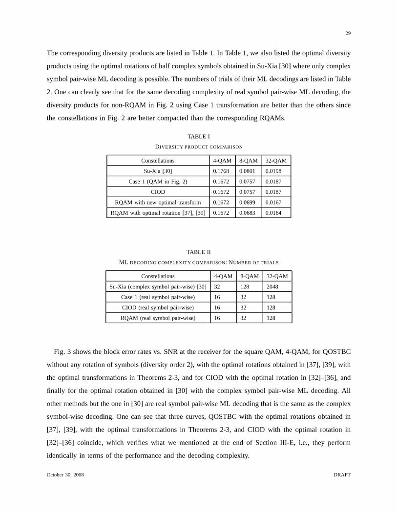
The corresponding diversity products are listed in Table 1.In Table 1, we also listed the optimal diversity

products using the optimal rotations of half complex symbols obtained in Su-Xia [30] where only complex

symbol pair-wise ML decoding is possible. The numbers of trials of their ML decodings are listed in Table

2. One can clearly see that for the same decoding complexity of real symbol pair-wise ML decoding, the

diversity products for non-RQAM in Fig. 2 using Case 1 transformation are better than the others since

the constellations in Fig. 2 are better compacted than the corresponding RQAMs.

TABLE I

DIVERSITY PRODUCT COMPARISON

Constellations 4-QAM 8-QAM 32-QAM

Su-Xia [30] 0.1768 0.0801 0.0198

Case 1 (QAM in Fig. 2) 0.1672 0.0757 0.0187

CIOD 0.1672 0.0757 0.0187

RQAM with new optimal transform 0.1672 0.0699 0.0167

RQAM with optimal rotation [37], [39] 0.1672 0.0683 0.0164

TABLE II

ML DECODING COMPLEXITY COMPARISON: NUMBER OF TRIALS

Constellations 4-QAM 8-QAM 32-QAM

Su-Xia (complex symbol pair-wise) [30] 32 128 2048

Case 1 (real symbol pair-wise) 16 32 128

CIOD (real symbol pair-wise) 16 32 128

RQAM (real symbol pair-wise) 16 32 128

Fig. 3 shows the block error rates vs. SNR at the receiver for the square QAM, 4-QAM, for QOSTBC

without any rotation of symbols (diversity order 2), with the optimal rotations obtained in [37], [39], with

the optimal transformations in Theorems 2-3, and for CIOD with the optimal rotation in [32]–[36], and

finally for the optimal rotation obtained in [30] with the complex symbol pair-wise ML decoding. All

other methods but the one in [30] are real symbol pair-wise MLdecoding that is the same as the complex

symbol-wise decoding. One can see that three curves, QOSTBCwith the optimal rotations obtained in

[37], [39], with the optimal transformations in Theorems 2-3, and CIOD with the optimal rotation in

[32]–[36] coincide, which verifies what we mentioned at the end of Section III-E, i.e., they perform

identically in terms of the performance and the decoding complexity.


30

10 11 12 13 14 15 16 17 18 19 2010

−5

10−4

10−3

10−2

10−1

QOSTBC and CIOD, 4 transmit and one receive antennas, 4QAM

SNR at the receiver (dB)

Blo

ck E

rror

Rat

e

QOSTBC no rotationQOSTBC with optimal rotation in [37,39]QOSTBC with new optimal transformationQOSTBC Su−Xia [30]CIOD with optimal rotation [35,36]

Fig. 3. Simulation results for schemes with the transmission rate of 2 bits/channel use.

The aim of Fig. 4 and Fig. 5 is to compare the performance between the newly obtained optimal

transformationsUi in Theorem 3 for both RQAM and non-RQAM (Case 1) with the optimal rotation

obtained in [37], [39] for RQAM. The block error rates vs. SNRat the receiver for 8-QAM (3 bits/s/Hz)

and 32-QAM (5 bits/s/Hz) are shown in Fig. 4 and Fig. 5, respectively. One can see that newly obtained

optimal transformationsUi in Theorem 3 for RQAM are better than the optimal rotation obtained in

[37], [39] for RQAM, and the newly obtained optimal transformation Ui for Case 1 in Theorems 2-3

for the non-RQAM constellations in Fig. 2 have the best performance when real symbol pair-wise ML

decoding is imposed. In Fig. 4 and Fig. 5, we also compare withthe optimal rotation obtained in [30]

with the complex symbol pair-wise ML decoding. All these results have confirmed the theoretical results

obtained and discussed in Sections II–III. Note that, for the QAM constellations generated fromsquare

QAM as shown in Fig. 2, the optimal rotation obtained in [37],[39] can achieve the same performance

as the optimal rotations for Case 1 in Theorems 2-3 do.

VI. CONCLUSIONS

In this paper, we systematically studied general linear transformations of information symbols for

QOSTBC to have both full diversity and real symbol pair-wiseML decoding. We presented necessary


31

8 10 12 14 16 18 20 22 2410

−5

10−4

10−3

10−2

10−1

100

QOSTBC, 4 transmit and one receive antennas, 8QAM


Blo

ck e

rror

rat

e

RQAM (N1=2, N

2=1), optimal rotation [37,39]

RQAM (N1=2, N

2=1), new optimal transform

8−QAM in Fig. 2(b), no rotation8−QAM in Fig. 2(b), Case 1 with new optimal transform8−QAM in Fig. 2(b), Su−Xia [30]


16 18 20 22 24 26 2810

−4

10−3

10−2

10−1

100

QOSTBC, 4 transmit and one receive antennas, 32QAM


Blo

ck e

rror

rat

e

RQAM (N1=4, N

2=2), optimal rotation [37,39]

RQAM (N1=4, N

2=2), new optimal transform

32−QAM in Fig. 2(a), no rotation32−QAM in Fig. 2(a), Case 1 with new optimal transform32−QAM in Fig. 2(a), Su−Xia [30]



32

and sufficient conditions on the linear transformations fora QOSTBC to possess a real symbol pair-

wise ML decoding. We then presented the optimal transformation matrices (among all possible linear

transformations not necessarily symbol rotations) of information symbols for QOSTBC with real symbol

pair-wise ML decoding such that the optimal diversity product is achieved for bothgeneralsquare QAM

and general rectangularQAM signal constellations. We showed that with our newly proposed optimal

linear transformations for QOSTB for RQAM in one of the threecases, i.e., Case 1, QOSTB has full

diversity and good diversity product property and real symbol pair-wise ML decoding for any finite signal

constellation on any lattice. Interestingly, the optimal diversity products for square QAM constellations

from the optimal linear transformations of information symbols found in this paper coincide with the

ones presented by Yuen-Guan-Tjhung by using their optimal rotations. However, the optimal diversity

products for non-square RQAM constellations from the optimal linear transformations of information

symbols found in this paper are better than the ones presented by Yuen-Guan-Tjhung by using their

optimal rotations. We also presented the optimal transformations for the co-ordinate interleaved orthogonal

designs (CIOD) proposed by Khan-Rajan for rectangular QAM constellations.

As a remark, in this paper, we assume MIMO channels are uncorrelated and no any feedback is used.

When MIMO channels are correlated, studies on QOSTBC can be found in, for example, [47]. When a

limited feedback is available, studies on OSTBC and QOSTBC can be found in, for example, [48]–[52].

Further recent developments on fast decoding and linear transformations can be found in, for example,

[41]–[44].

APPENDIX

In this appendix, we prove Theorems 1, 2, 3 and 6. To do so, let us first see a lemma.

Lemma 1. Let A be a real4 × 4 symmetry matrix andS ⊂ R2 be a subset of two dimensional real

spaceR2. Assume that there are at least4 points inS such that they are not collinear. If for any real

number pairs(x1, y1), (x2, y2) ∈ S,

(

x1 y1 x2 y2

)

A

x1

y1

x2

y2

= 0,

then,A = 0.


33

Proof: Assume(xi, yi) ∈ S, i = 1, 2, 3, 4, are not collinear. SinceA is a real symmetric matrix,A has

a diagonalized formA = V tDV , whereV is an orthogonal matrix andD = diag(µ1, µ2, µ3, µ4) with

real µi. To prove Lemma 1, it is enough to prove thatµ1 = µ2 = µ3 = µ4 = 0.

From the condition of the lemma,

(xi, yi, xj, yj)VtDV (xi, yi, xj , yj)

t = 0,

for any 1 ≤ i, j ≤ 4. Thus, if there existi, j such that the first component of vectorV (xi, yi, xj , yj)t

is not 0, thenµ1 = 0 is proved. To show so, let us use the contradiction method. Assume that for any

i, j, 1 ≤ i, j ≤ 4, the first component ofV (xi, yi, xj , yj)t is 0. Denote the first row of matrixV as

(v1, v2, v3, v4). Then

(v1, v2, v3, v4)(xi, yi, xj , yj)t = 0.

Consideringi = 1 andj = 1, we have

(v1, v2, v3, v4)(x1, y1, x1, y1)t = 0.

Consideringi = 2 andj = 1, we have

(v1, v2, v3, v4)(x2, y2, x1, y1)t = 0.

Therefore,

(v1, v2, v3, v4)(x1 − x2, y1 − y2, 0, 0)t = 0,

i.e.,

v1(x1 − x2) + v2(y1 − y2) = 0.

Similarly, we have

v1(x1 − x3) + v2(y1 − y3) = 0 and v1(x1 − x4) + v2(y1 − y4) = 0.

If (v1, v2) 6= 0, the the above three equations imply that the four points(x1, y1), (x2, y2), (x3, y3) and

(x4, y4) are collinear, which contradicts with the assumption in thebeginning of the proof. Thus, we have

proved(v1, v2) = 0. Similarly, we can provev3 = v4 = 0. This means that the first row of orthogonal

matrix V is the all zero vector, which is impossible. Therefore, we have proved that there existi, j

such that the first component ofV (xi, yi, xj , yj)t is not 0. Hence,µ1 = 0. Similarly, we can prove

µ2 = µ3 = µ4 = 0. q.e.d.


34

Proof of Theorem 1

We first consider Case 1. Considerfi in (20) and its representation in (25). Clearly,fi is a quadratic

form of the variablesri, si, rk+i, sk+i and hence iffi can be separated as

fi(ri, si, rk+i, sk+i) = fi1(ri, si) + fi2(rk+i, sk+i),

then,fi1 andfi2 are also quadratic forms ofri, si andrk+i, sk+i, respectively. Therefore, there exist two

real 2 × 2 symmetric matricesAi1 andAi2, such that

fi1(ri, si) = (ri, si)Ai1

ri

si

andfi2(rk+i, sk+i) = (rk+i, sk+i)Ai2

rk+i

sk+i

. (68)

Combining with (25), we have

(ri, si, rk+i, sk+i)Uti

0 I2

I2 0

Ui

ri

si

rk+i

sk+i

= (ri, si)Ai1

ri

si

+ (rk+i, sk+i)Ai2

rk+i

sk+i

.

(69)

Letting Ui =

Ui1 Ui2

Ui3 Ui4

and rewriting (69), we have

(ri, si, rk+i, sk+i)

U ti1Ui3 + U t

i3Ui1 − Ai1 U ti3Ui2 + U t

i1U4i

(U ti3Ui2 + U t

i1Ui4)t U t

i2Ui4 + U ti4Ui2 − Ai2

ri

si

rk+i

sk+i

= 0. (70)

Therefore, by Lemma 1,fi can be separated as a sum of two functions as Case 1 if and only if

U ti3Ui2 + U t

i1Ui4 = 0. (71)

Doing the similar calculations for functiongi in (19) and (24), we have that functionsgi can be separated

as a sum of two functions as Case 1 if and only if

U ti1Ui2 + U t

i3Ui4 = 0. (72)

Thus,

Ui2

Ui4

t

Ui1

Ui3

= 0 and

Ui2

Ui4

t

Ui3

Ui1

= 0. (73)


35

SinceUi is non-singular and thus, the column vectors of matrix

Ui2

Ui4

are linearly independent and so

are true for matrices

Ui1

Ui3

and

Ui3

Ui1

. The first equation in (73) tells us that the two dimensional

real space spanned by the column vectors of

Ui1

Ui3

is the complimentary space of the one spanned

by the column vectors of

Ui2

Ui4

in the four dimensional real space. The second equation in (73)

also tells us that the two dimensional real space spanned by the column vectors of

Ui3

Ui1

is the

complimentary space of the one spanned by the column vectorsof

Ui2

Ui4

in the four dimensional

real space. Thus, the two dimensional real space spanned by the column vectors of

Ui1

Ui3

is the

same as the one spanned by the column vectors of

Ui3

Ui1

. This means that there exists a2× 2 (real)

non-singular matrixRi1 such that

Ui3

Ui1

=

Ui1

Ui3

Ri1,

i.e.,

Ui3 = Ui1Ri1 andUi1 = Ui3Ri1. (74)

Therefore,

Ui1

Ui3

=

Ui3

Ui1

Ri1 =

Ui1Ri1

Ui3Ri1

Ri1 =

Ui1

Ui3

R2i1.

Again, by the linear independence of the two columns of matrix

Ui1

Ui3

, we have

R2i1 = I2. (75)

Similarly, we can obtain the results for

Ui2

Ui4

. Thus, we have proved (i) for Case 1 in Theorem 1.


36

For (ii) for Case 2, it is enough to note that

fi(ri, si, rk+i, sk+i) = (ri, rk+i, si, sk+i)(UiP1)t

0 I2

I2 0

(UiP1)

ri

rk+i

si

sk+i

and

gi(ri, si, rk+i, sk+i) = (ri, rk+i, si, sk+i)(UiP1)t

I2 0

0 I2

(UiP1)

ri

rk+i

si

sk+i

Then, all results can be derived ifUi is replaced byUiP1 as in (i) for Case 1.

The proof of (iii) for Case 3 is similar to the one of (ii) for Case 2. q.e.d.

Proof of Theorem 2

Let ri + jsi and r′i + js′i, i = 1, 2, · · · , k, k + 1, · · · , 2k, be symbols taken from a square-QAM and

denote∆ri = ri−r′i and∆si = si−s′i. The transmitted symbols are obtained through the transformations

(18):

(pi, qi, pk+i, qk+i)t = Ui(ri, si, rk+i, sk+i)

t; (p′i, q′i, p

′k+i, q

′k+i)

t = Ui(r′i, s

′i, r

′k+i, s

′k+i)

t. (76)

Denote∆pi = pi − p′i and∆qi = qi − q′i. Then,

(∆pi,∆qi,∆pk+i,∆qk+i)t = Ui(∆ri,∆si,∆rk+i,∆sk+i)

t, (77)

and

det((∆C)†(∆C)) = det

(∆a)In (∆b)In

(∆b)In (∆a)In

,

where∆a =∑2k

i=1(∆pi)2 +

∑ki=1(∆qi)

2 and∆b = 2∑k

i=1(∆pi∆pk+i + ∆qi∆qk+i). And,

det

(∆a)In (∆b)In

(∆b)In (∆a)In

= [(∆a)2 − (∆b)2]n = (∆a + ∆b)n(∆a − ∆b)n. (78)

In the rest of this proof, since a QOSTBC is linear in terms of variablesri, si, pi, qi and their differences

are also integers, for simplicity we omit the notation∆. For convenience, we also denote

Dmin∆= min

(x1,··· ,x2k)6=(x′

1,··· ,x′

2k)det((∆C)†(∆C)),


37

wherexi = pi + jqi andx′i = p′i + jq′i. Thus, the diversity product of a QOSTCQ2n can be expressed as

ζ(Q2n) =1

2√

2T(Dmin)

1

4n .

Let us first consider (i) for Case 1 in Theorem 2. By the definitions of∆a and∆b, we have

∆a + ∆b

=k∑

i=1

(pi, qi, pk+i, qk+i)

I2 I2

I2 I2

pi

qi

pk+i

qk+i

=

k∑

i=1

(ri, si, rk+i, sk+i)Uti

I2 I2

I2 I2

Ui

ri

si

rk+i

sk+i

=k∑

i=1


Ui1 Ui2

Ui1Ri1 Ui2Ri2

t

I2 I2

I2 I2

Ui1 Ui2

Ui1Ri1 Ui2Ri2

ri

si

rk+i

sk+i

=

k∑

i=1


Ki1 Ki2

Kti2 Ki3

ri

si

rk+i

sk+i

(79)

where

Ki1 = U ti1Ui1 + Rt

i1Uti1Ui1 + U t

i1Ui1Ri1 + Rti1U

ti1Ui1Ri1,

Ki2 = U ti1Ui2 + Rt

i1Uti1Ui2 + U t

i1Ui2Ri2 + Rti1U

ti1Ui2Ri2,

Ki3 = U ti2Ui2 + Rt

i2Uti2Ui2 + U t

i2Ui2Ri2 + Rti2U

ti2Ui2Ri2.

By (27) andR2i1 = R2

i2 = I2, we know thatKi2 = 0. Therefore,

∆a + ∆b =

k∑

i=1

(ri, si)Ki1

ri

si

+

k∑

i=1

(rk+i, sk+i)Ki3

rk+i

sk+i

. (80)


38

For anyi, i = 1, 2 · · · , k,

(ri, si)Ki1

ri

si

=1

2(ri, si, ri, si)

Ui1 Ui1Ri1

Ui1Ri1 Ui1

t

Ui1 Ui1Ri1

Ui1Ri1 Ui1

ri

si

ri

si

.

Hence,

(ri, si)Ki1

ri

si

≥ 0,

andKi1, i = 1, 2 · · · , k, are non-negative definite. Similarly,Ki3, i = 1, 2 · · · , k, are also non-negative

definite. Therefore, for any fixed indexi, i ∈ 1, 2, · · · , k,

∆a + ∆b ≥ (ri, si)Ki1

ri

si

and∆a + ∆b ≥ (rk+i, sk+i)Ki3

rk+i

sk+i

. (81)

Similar,

∆a − ∆b =

k∑

i=1


Ki1 0

0 Ki3

ri

si

rk+i

sk+i

(82)

=

k∑

i=1

(ri, si)Ki1

ri

si

+

k∑

i=1

(rk+i, sk+i)Ki3

rk+i

sk+i

(83)

where

Ki1 = U ti1Ui1 − Rt

i1Uti1Ui1 − U t

i1Ui1Ri1 + Rti1U

ti1Ui1Ri1,

Ki3 = U ti2Ui2 − Rt

i2Uti2Ui2 − U t

i2Ui2Ri2 + Rti2U

ti2Ui2Ri2.

Also for any i, i = 1, 2, · · · , k,


39

(ri, si)Ki1

ri

si

=1

2(ri, si, ri, si)

Ui1 −Ui1Ri1

−Ui1Ri1 Ui1

t

Ui1 −Ui1Ri1

−Ui1Ri1 Ui1

ri

si

ri

si

.

Hence,

(ri, si)Ki1

ri

si

≥ 0,

andKi1, i = 1, 2 · · · , k, are non-negative definite. Similarly,Ki3, i = 1, 2 · · · , k, are non-negative definite

too. Therefore, for any fixed indexi, i ∈ 1, 2, · · · , k,

∆a − ∆b ≥ (ri, si)Ki1

ri

si

and∆a − ∆b ≥ (rk+i, sk+i)Ki3

rk+i

sk+i

. (84)

Summarizing the above results, we have

det

(∆a)In (∆b)In

(∆b)In (∆a)In

≥

(ri, si)Ki1

ri

si

(ri, si)Ki1

ri

si

n

, (85)

det

(∆a)In (∆b)In

(∆b)In (∆a)In

≥

(rk+i, sk+i)Ki3

rk+i

sk+i

(rk+i, sk+i)Ki3

rk+i

sk+i

n

, (86)

for any indexi, i = 1, 2, · · · , k, which gives lower bounds of the determinant. Sinceri, si, i = 1, · · · , 2k,

are independent integers, these lower bounds can be achieved by letting rt = st = 0 for t 6= i. Hence,

the minimum of (85) or (86) for0 6= (ri, si) ∈ Z × Z is the minimum of the determinant, i.e.,

Dmin = mini∈1,2,··· ,k

min06=(rt,st)∈Z×Z

(rt, st)Si

rt

st

(rt, st)Si

rt

st

n

. (87)

where(Si, Si) can be(Ki1, Ki1) or (Ki3, Ki3) that are non-negative definite.

We next want to have an upper bound forDmin. To do so, we need the following lemma, which can

be found in pp. 83, [54].

Lemma 2. Let ξ = αx + βy, η = γx + δy, and |αδ − βγ|2 = ∆ > 0, wherex and y are integers. Then,

for the indefinite binary quadratic formf = ξη with discriminant∆, there exists a point(x, y) 6= 0 such

that

|ξη| = |f(x, y)| ≤√

∆

5. (88)


40

To use this lemma, we need to change

(ri, si)Si

ri

si

(ri, si)Si

ri

si

(89)

into a product of two linear forms. To do so, it is enough to consider the case whenSi = Ki1 and

Si = Ki1 and the other case is the same.

From R2i1 = I2, we haveRi1 = ±I2 or

Ri1 =

ai1 bi1

ci1 −ai1

,

whereai1, bi1, ci1 are real numbers and subject to the following condition

a2i1 + bi1ci1 = 1. (90)

We next make some assumptions to partially prove the result we wanted, and then we fully prove the

result by removing the assumptions.

First, we assume Assumption 1:Ri1 6= ±I2. Let Rti1U

ti1Ui1 + U t

i1Ui1Ri1∆=

ki1 ki2

ki2 ki3

. Then

(ri1, si1)Ki1

ri1

si1

= (ri1, si1)(Uti1Ui1 + Rt

i1Uti1Ui1Ri1 + Rt

i1Uti1Ui1 + U t

i1Ui1Ri1)

ri1

si1

= (ri1, si1)(Rti1(R

ti1U

ti1Ui1 + U t

i1Ui1Ri1) + Rti1U

ti1Ui1 + U t

i1Ui1Ri1)

ri1

si1

= (ri1, si1)

ai1 bi1

ci1 −ai1

t

ki1 ki2

ki2 ki3

+

ki1 ki2

ki2 ki3

ri1

si1

= (ri1, si1)

(1 + ai1)ki1 + ci1ki2 (1 + ai1)ki2 + ci1ki3

bi1ki1 + (1 − ai1)ki2 bi1ki2 + (1 − ai1)ki3

ri1

si1

. (91)

Note thatKi1 is a non-negative definite (symmetry) matrix. Thus,(1 + ai1)ki1 + ci1ki2 ≥ 0, and

(1 + ai1)ki2 + ci1ki3 = bi1ki1 + (1 − ai1)ki2. (92)

Assume Assumption 2:(1 + ai1)ki1 + ci1ki2 > 0. Then, using (90) and (92), we have

(ri1, si1)Ki1

ri1

si1

=

(

√

(1 + ai1)ki1 + ci1ki2 ri1 +(1 + ai1)ki2 + ci1ki3√

(1 + ai1)ki1 + ci1ki2

si1

)2

(93)


41

Similarly, for Ki1 we have

(ri1, si1)Ki1

ri1

si1

= (ri1, si1)(Uti1Ui1 + Rt

i1Uti1Ui1Ri1 − Rt

i1Uti1Ui1 − U t

i1Ui1Ri1)

ri1

si1

= (ri1, si1)

ai1 bi1

ci1 −ai1

t

ki1 ki2

ki2 ki3

−

ki1 ki2

ki2 ki3

ri1

si1

= (ri1, si1)

(ai1 − 1)ki1 + ci1ki2 (ai1 − 1)ki2 + ci1ki3

bi1ki1 − (ai1 + 1)ki2 bi1ki2 − (ai1 + 1)ki3

ri1

si1

(94)

Also note thatKi1 is a non-negative definite (symmetry) matrix and thus(ai1 − 1)ki1 + ci1ki2 ≥ 0.

Assume Assumption 3:(ai1 − 1)ki1 + ci1ki2 > 0. Then,

(ri1, si1)Ki1

ri1

si1

=

(

√

(ai1 − 1)ki1 + ci1ki2 ri1 +(ai1 − 1)ki2 + ci1ki3√

(ai1 − 1)ki1 + ci1ki2

si1

)2

. (95)

Therefore, (89) can be rewritten into the following squaredproduct of two linear forms:

(ri1, si1)Ki1

ri1

si1

(ri1, si1)Ki1

ri1

si1

=

(

√

(1 + ai1)ki1 + ci1ki2 ri1 +(1 + ai1)ki2 + ci1ki3√

(1 + ai1)ki1 + ci1ki2

si1

)2

×(

√

(ai1 − 1)ki1 + ci1ki2 ri1 +(ai1 − 1)ki2 + ci1ki3√

(ai1 − 1)ki1 + ci1ki2

si1

)2

(96)

Let

α =√

(1 + ai1)ki1 + ci1ki2, β =(1 + ai1)ki2 + ci1ki3√

(1 + ai1)ki1 + ci1ki2

,

γ =√

(ai1 − 1)ki1 + ci1ki2, δ =(ai1 − 1)ki2 + ci1ki3√

(ai1 − 1)ki1 + ci1ki2

.

By Assumptions 2 and 3,(1 + ai1)ki1 + ci1ki2 > 0 and (ai1 − 1)ki1 + ci1ki2 > 0, and using (90),we

conclude thatci1 6= 0. Thus, by using (90) and (92), the discriminant is

∆i = (αδ − βγ)2 = 4(ki2 +ai1 + 1

ci1ki1)(ki2 +

ai1 − 1

ci1ki1) > 0. (97)

By Lemma 2, we have

Dmin ≤ mini∈1,2,··· ,k

(∆i

5)n = min

i∈1,2,··· ,k

4

5

(

ki2 +ai1 + 1

ci1ki1)(ki2 +

ai1 − 1

ci1ki1

)n

. (98)


42

We next begin to remove the three assumptions: Assumption 1,Ri1 6= ±I2; Assumption 2,(1 +

ai1)ki1 + ci1ki2 > 0; and Assumption 3,(ai1 − 1)ki1 + ci1ki2 > 0.

For Assumption 1, ifRi1 = I, then Ki1 = 0 from the definition ofKi1. Using (87), we know that

Dmin = 0. So (98) is true. IfRi1 = −I2, thenKi1 = 0 and (98) is also true.

For Assumption 2, if(1 + ai1)ki1 + ci1ki2 = 0, then from (91),

(ri1, si1)Ki1

ri1

si1

= (ri1, si1)

0 (1 + ai1)ki2 + ci1ki3

bi1ki1 + (1 − ai1)ki2 bi1ki2 + (1 − ai1)ki3

ri1

si1

.

Letting ri1 = 1 andsi1 = 0, we have(ri1, si1)Ki1

ri1

si1

= 0. Going back to (87), we haveDmin = 0.

Hence, (98) is still true. The same method can be used to remove Assumption 3. Therefore, the upper

bound formula (98) is always true.

To derive an upper bound of the normalized diversity productζ(Q2n) in (38), we need to calculate

the determinant

det(U1) det(U2) · · · det(Uk).

Let us seedet(Ui):

(det(Ui))2 = det(U t

i Ui) = det

Ui1 Ui2

Ui1Ri1 Ui2Ri2

t

Ui1 Ui2

Ui1Ri1 Ui2Ri2

= det

U ti1Ui1 + Rt

i1Uti1Ui1Ri1 0

0 U ti2Ui2 + Rt

i2Uti2Ui2Ri2

= det(U ti1Ui1 + Rt

i1Uti1Ui1Ri1) det(U t

i2Ui2 + Rti2U

ti2Ui2Ri2)

= det(Rti1) det

ki1 ki2

ki2 ki3

det(Rti2) det

li1 li2

li2 li3

where the third equality comes from (27) andR2i1 = I2 and in the last equality, we denote that

li1 li2

li2 li3

∆= Rt

i2Uti2Ui2 + U t

i2Ui2Ri2.

For lij andRi2, similar properties as (90), (92), and (98) also hold. Againby R2i1 = R2

i2 = I2, we have

|det(Ri1)| = |det(Ri2)| = 1. Therefore,

(det(Ui))2 = |ki1ki3 − k2

i2| |li1li3 − l2i2|. (99)


43

and

|k∏

i=1

det(Ui)| =

√

√

√

√

k∏

i=1

|ki1ki3 − k2i2|

k∏

i=1

|li1li3 − l2i2|. (100)

We assume that

|ki01ki03 − k2i02| = min

i=1,2,··· ,k

|ki1ki3 − k2i2|, |li1li3 − l2i2|

. (101)

Then

|k∏

i=1

det(Ui)| ≥ |ki01ki03 − k2i02|k (102)

By the definition ofζ(Q2n) in (38), (98) and (102) forkij or lij, we obtain the following upper bound:

ζ(Q2n) ≤ 1

2√

2T(4

5)

1

4

|(ki02 +ai01+1

ci01ki01)(ki02 +

ai01−1ci01

ki01)||ki01ki03 − k2

i02|

1/4

. (103)

On the other hand, from (90) and (92), it is not hard to see that

|ki01ki03 − k2i02| = |(ki02 +

ai01 + 1

ci01ki01)(ki02 +

ai01 − 1

ci01ki01)|.

Thus, we obtain the following upper bound onζ(Q2n):

ζ(Q2n) ≤ 1

2√

2T(4

5)1/4. (104)

Next, we show that if we letUi1 = Ui2 = 1√2I2 and

Ri1 = −Ri2 = R =

cos(θ) sin(θ)

sin(θ) − cos(θ)

,

whereθ = arctan(2), then ζ(Q2n) achieves the above upper bound.

By letting ai1 = cos(θ), bi1 = ci1 = sin(θ), we know thatUi are orthogonal matrices. By the definitions

in (79) and (83), we know thatKi1 = I2 + R andKi1 = I2 − R. Thus, from (87), we have

Dmin = min06=(r,s)∈Z×Z

(

(r, s)(I2 + R)(r, s)t(r, s)(I2 − R)(r, s)t)n

= min06=(r,s)∈Z×Z

[(1 + cos(θ))r2 + 2 sin(θ)rs + (1 − cos(θ))s2]n

× [(1 − cos(θ))r2 − 2 sin(θ)rs + (1 + cos(θ))s2]n


(

4[cos(θ/2)r + sin(θ/2)s]2[sin(θ/2)r − cos(θ/2)s]2)n


(

[sin(θ)r2 − 2 cos(θ)rs − sin(θ)s2]2)n

= (sin2(θ))n min06=(r,s)∈Z×Z

(

[r2 − rs − s2]2)n

, (105)

where the last equality comes fromtan(θ) = 2, i.e., sin(θ) = 2 cos(θ).


44

Sincer ands are integers and(r, s) 6= 0, we have[r2 − rs− s2]2 ≥ 1. If we let r = 1 ands = 0, we

have[r2 − rs − s2]2 = 1. Therefore,Dmin = (sin2(θ))n. But sin2(θ) = 45 , and hence

Dmin = (4

5)n. (106)

On the other hand, sinceUi are orthogonal matrices, we have|det(Ui)| = 1. Therefore, we obtain

ζ(Q2n) =1

2√

2T(4

5)1/4. (107)

This proves (i) for Case 1 in Theorem 2.

If in the above proof, we replaceUi by UiP1, we can similarly prove (ii) for Case 2, and if we replace

Ui by UiP2, we can prove (iii) for Case 3, in Theorem 2. q.e.d.

Proof of Theorem 3

We inherit all the notations in the above proof of Theorem 2. Similar to the proof of Theorem 2,

we evaluateDmin and obtain an upper bound, and then show that this upper boundcan be achieved.

Unfortunately, the result for indefinite binary quadratic forms in Lemma 2 can not be applied here for

finite signal constellations.

By checking formulas from (76) to (87) and from (89) to (96), we find that these formulas are all true

under the conditions of Theorem 3. Especially, (87) and (96)are true and the three assumptions in the

proof of Theorem 2 can be removed too. Let us recalculate

(ri, si)Ki1

ri

si

(ri, si)Ki1

ri

si

(108)

under the conditions of Theorem 3. Continuing with (96) and using a2i1 + bi1ci1 = 1 and ci1ki3 =

bi1ki1 − 2ai1ki2 from (92), we have

(ri, si)Ki1

ri

si

(ri, si)Ki1

ri

si

= (k2i2 + 2

ai1

ci1ki1ki2 −

bi1

ci1k2

i1)(ci1r2i − 2ai1ri1si1 − bi1s

2i )

2. (109)

Since

k2i2 − ki1ki3 = k2

i2 − ki11

ci1(bi1ki1 − 2ai1ki2) = k2

i2 + 2ai1

ci1ki1ki2 −

bi1

ci1k2

i1,

we have

(ri, si)Ki1

ri

si

(ri, si)Ki1

ri

si

= (k2i1 − ki1ki3)(ci1r

2i − 2ai1ri1si1 − bi1s

2i )

2. (110)


45

On the other hand,

ki1ki3 − k2i2 = det

ki1 ki2

ki2 ki3

= det(Rti1U

ti1Ui1 + U t

i1Ui1Ri1) = det(Rti1) det(U t

i1Ui1 + Rti1U

ti1Ui1Ri1)

= − det(U ti1Ui1 + Rt

i1Uti1Ui1Ri1) (111)

where the second equality is from the definition ofkij in the proof of Theorem 2, and the last equality

is from the facts that

Ri1 =

ai1 bi1

ci1 −ai1

anda2i1 + bi1ci1 = 1.

Consequently, (110) can be changed into

(ri, si)Ki1

ri

si

(ri, si)Ki1

ri

si

= det(U ti1Ui1 + Rt

i1Uti1Ui1Ri1)(ci1r

2i − 2ai1ri1si1 − bi1s

2i )

2. (112)

Note that the above calculations are also true for(Ki3, Ki3), and thus (112) holds if the subscript1 in

(112) is replaced by2. Hence, going back to (87), we obtain

Dmin = mini∈1,2,··· ,k

min06=(r,s)∈∆RQAM

minj=1,2

det(U tijUij + Rt

ijUtijUijRij)(cijr

2 − 2aijrs − bijs2)2n

(113)

where∆RQAM∆= (r1 − r2, s1 − s2) | r1 + js1 ∈ RQAM; r2 + js2 ∈ RQAM. From the form of an

RQAM in (8)-(9), one can see that for(r, s) ∈ ∆RQAM, r ands must be integer multiples ofd.

Let us first evaluate determinantdet(U tijUij +Rt

ijUtijUijRij). We now need the energy constraint (47).

Without loss of generality, we may assume that

∑

ru+jsu∈RQAM

(ru, su)(U tu1Uu1 + Rt

u1Utu1Uu1Ru1)

ru

su

≤∑

ri+jsi∈RQAM(ri, si)(U

tijUij + Rt

ijUtijUijRij)

ri

si

, 1 ≤ i ≤ k, j = 1, 2.

Then, from (47), we have

0 ≤∑

ru+jsu∈RQAM(ru, su)(U t

u1Uu1 + Rtu1U

tu1Uu1Ru1)

ru

su

≤ 1. (114)


46

From the definition

ku1 ku2

ku2 ku3

= Rtu1U

tu1Uu1 + U t

u1Uu1Ru1 andR2u1 = I2, we have

U tu1Uu1 + Rt

u1Utu1Uu1Ru1 = Rt

u1(Rtu1U

tu1Uu1 + U t

u1Uu1Ru1)

=

au1 cu1

bu1 −au1

ku1 ku2

ku2 ku3

=

au1ku1 + cu1ku2 au1ku2 + cu1ku3

bu1ku1 − au1ku2 bu1ku2 − au1ku3

. (115)

Note that the above matrix is symmetric, we haveau1ku2 + cu1ku3 = bu1ku1 − au1ku2, and (114) can be

changed into

(au1ku1 + cu1ku2)∑

ru+jsu∈RQAMr2u

+ 2(au1ku2 + cu1ku3)∑

ru+jsu∈RQAM

rusu + (bu1ku2 − au1ku3)∑

ru+jsu∈RQAM

s2u ≤ 1. (116)

Because

∑

ru+jsu∈RQAM

r2u = N2(

4N31

3− N1

3)d2 =

4N21 − 1

2(2N21 + 2N2

2 − 1)

∆= ε1, (117)

∑

ru+jsu∈RQAMs2u = N1(

4N32

3− N2

3)d2 =

4N22 − 1

2(2N21 + 2N2

2 − 1)

∆= ε2, (118)

and∑

ru+jsu∈RQAM rusu = 0, (116) becomes

0 ≤ ε1(au1ku1 + cu1ku2) + ε2(bu1ku2 − au1ku3) ≤ 1. (119)

From 2au1ku2 = bu1ku1 − cu1ku3, the energy constraint (114) becomes

0 ≤ (a2u1 + 1)ε1 + b2

u1ε2

2au1ku1 −

c2u1ε1 + (a2

u1 + 1)ε2

2au1ku3 ≤ 1. (120)

Now we can evaluate determinantdet(U tu1Uu1 + Rt

u1Utu1Uu1Ru1). From (111), and2au1ku2 = bu1ku1 −

cu1ku3, we have

det(U tu1Uu1 + Rt

u1Utu1Uu1Ru1) = k2

u2 − ku1ku3 =b2u1k

2u1 − 2(a2

u1 + 1)ku1ku3 + c2u1k

2u3

4a2u1

, (121)

where we have assumed thatau1 6= 0. The case whenau1 = 0 will be considered later.

Using Lagrange multipliers, we can obtain the upper bound ofdet(U tu1Uu1 + Rt

u1Utu1Uu1Ru1) under

condition (120):

0 ≤ det(U tu1Uu1 + Rt

u1Utu1Uu1Ru1) = k2

u2 − ku1ku3 ≤ 1

(bu1ε2 − cu1ε1)2 + 4ε1ε2. (122)


47

Combining it with (113), we have

Dmin ≤ min06=(r,s)∈∆RQAM

(cu1r2 − 2au1rs − bu1s

2)2

(bu1ε2 − cu1ε1)2 + 4ε1ε2

n

. (123)

Since(d, 0) ∈ ∆RQAM, (0, d) ∈ ∆RQAM and (d, d) ∈ ∆RQAM,

min06=(r,s)∈∆RQAM

(cu1r2 − 2au1rs − bu1s

2)2 ≤ minb2u1d

4, c2u1d

4, (cu1 − 2au1 − bu1)2d4.

Therefore,

Dmin ≤

minb2u1d

4, c2u1d

4, (cu1 − 2au1 − bu1)2d4

(bu1ε2 − cu1ε1)2 + 4ε1ε2

n

. (124)

It is not hard to prove that under conditionsa2u1 + bu1cu1 = 1 andε1 +ε2 = 1 that is from the definitions

of ε1 andε2 in Theorem 3, whenb2u1 = c2

u1 = (cu1 − 2au1 − bu1)2, i.e., b2

u1 = c2u1 = 4a2

u1 = 45 , the right

hand side of (124) achieves the maximum. Therefore, we have

Dmin ≤

d4

1 + ε1ε2

n

. (125)

We now consider the case whenau1 = 0. If au1 = 0, thenbu1cu1 = 1 from the fact thata2u1 +bu1cu1 = 1

and the energy constraint (119) becomes

(cu1ε1 + bu1ε2)ku2 ≤ 1. (126)

On the other hand, from (115),

U tu1Uu1 + Rt

u1Utu1Uu1Ru1 =

cu1ku2 cu1ku3

bu1ku1 bu1ku2

.

Since the left hand side of the above equation is non-negative definite, we havecu1ku2 ≥ 0 andbu1ku2 ≥0.

Sinceε1 > 0, ε2 > 0 andbu1cu1 = 1, we havecu1ε1 + bu1ε2 6= 0. Hence, combiningcu1ku2 ≥ 0 and

bu1ku2 ≥ 0 with inequality (126) andε1 > 0, ε2 > 0, we obtain that the left hand side of inequality

(126) is positive and

k2u2 ≤

(

1

cu1ε1 + bu1ε2

)2

.

Consequently,

det(U tu1Uu1 + Rt

u1Utu1Uu1Ru1)

= k2u2 − ku1ku3 = k2

u2 − ku1(bu1

cu1ku1) = k2

u2 − k2u1

bu1cu1

c2u1

≤ k2u2 ≤

(

1

cu1ε1 + bu1ε2

)2

≤ 1

(bu1ε2 − cu1ε1)2 + 4ε1ε2,


48

where the first equality comes from (121), and the second equality comes from bu1ku1 − cu1ku3 =

2au1ku2 = 0, and the first inequality is frombu1cu1 = 1, and the last inequality is also due tobu1cu1 = 1

andε1 > 0, ε2 > 0. Therefore, (122) is also true whenau1 = 0, and so is the upper bound formula (125).

With the upper bound (125) onDmin, we next prove that this upper bound is achievable. To do so, it

is enough to construct matricesUi such that this bound is achieved.

For a fixed RQAM, the numbersN1, N2 andε1, ε2 with ε1 + ε2 = 1 are fixed. Letα = arctan(2) and

ρ =√

512(1+ε1ε2)

. Let the matricesR,P,Σ be

R =

cos(α) sin(α)

sin(α) − cos(α)

, P =

0 1

1 0

, Σ =

1 + ε1 1 − 2ε1

1 − 2ε1 2 − ε1

. (127)

Clearly, Rt = R,R2 = I2 andP 2 = I2. Because0 < ε1 < 1, Σ is symmetric and positive definite. So,

Σ has a diagonal decompositionΣ = V tDV , whereD = diag(λ1, λ2), λ1, λ2 are the eigenvalues ofΣ,

V is an orthogonal matrix.

Let Ui1 = ρV t√

DV for i = 1, 2, · · · , k andUi2 = ρV tdiag(√

λ2,√

λ1)V P for i = 1, 2, · · · , k. Then,

U ti1Ui1 = ρ2Σ andU t

i2Ui2 = ρ2PV tdiag(λ2, λ1)V P . Let Ri1 = R andRi2 = −PRP for i = 1, 2, · · · , k.

ThenR2i1 = R2 = I2, R2

i2 = PR2P = I2, and

Rti1U

ti1Ui2 + U t

i1Ui2Ri2

= ρ2RV t

√λ1 0

0√

λ2

V · V t

√λ2 0

0√

λ1

V P

+ ρ2V t

√λ1 0

0√

λ2

V · V t

√λ2 0

0√

λ1

V P (−PRP )

= ρ2√

λ1λ2(RP − RP ) = 0.

Therefore, the conditions in (i) for Case 1 in Theorem 1 are satisfied.

We next calculate the minimum determinantDmin by using (113). Since, for anyi ∈ 1, 2, · · · , k, j =

1,

det(U tijUij + Rt

ijUtijUijRij)(cijr

2 − 2aijrs − bijs2)2

= ρ4 det(Σ + RΣR)(4

5)(r2 − rs − s2)2 =

(r2 − rs − s2)2

1 + ε1ε2. (128)

For j = 2, we want to show

det(U tijUij + Rt

ijUtijUijRij)(cijr

2 − 2aijrs − bijs2)2 =

(−r2 − rs + s2)2

1 + ε1ε2. (129)


49

To do so, we first show

det(U ti2Ui2 + Rt

i2Uti2UijRi2) = det(U t

i1Ui1 + Rti1U

ti1Ui1Ri1). (130)

From the definitions ofUi2 andRi2,

det(U ti2Ui2 + Rt

i2Uti2Ui2Ri2)

= det(ρ2PV tdiag(λ2, λ1)V P + (−PRP )(ρ2PV tdiag(λ1, λ2)V P )(−PRP )

= ρ4 det(V tdiag(λ2, λ1)V + RV tdiag(λ2, λ1)V R).

Note thatdet(U ti1Ui1+Rt

i1Uti1Ui1Ri1) = ρ4 det(V tdiag(λ1, λ2)V +RV tdiag(λ1, λ2)V R). Thus, to prove

(130), it is enough to prove

det(V tdiag(λ2, λ1)V + RV tdiag(λ2, λ1)V R) = det(V tdiag(λ1, λ2)V + RV tdiag(λ1, λ2)V R).

Denote the matrices inside the determinant signs of the leftand the right hand sides of the above equation

by M1 andM2, respectively. Then,

M1 + M2 = V tdiag(λ1 + λ2, λ2 + λ1)V + RV tdiag(λ1 + λ2, λ2 + λ1)V R

= 2(λ1 + λ2)I2.

If we denoteM1 =

m1 m2

m2 m3

, then,

det(M2) = det(2(λ1 + λ2)I2 − M1) =

2(λ1 + λ2) − m1 −m2

−m2 2(λ1 + λ2) − m3

= [2(λ1 + λ2) − m1][2(λ1 + λ2) − m3] − m22

= 4(λ1 + λ2)2 − 2(m1 + m3)(λ1 + λ2) + m1m3 − m2

2

= 4(λ1 + λ2)2 − 2tr(M1)(λ1 + λ2) + det(M1)

= 4(λ1 + λ2)2 − 2(2(λ1 + λ2))(λ1 + λ2) + det(M1) = det(M1),

where we use the fact thattr(M1) = 2(λ1 + λ2). Thus, we have proved (130). From (130) and (128),

we have (129).

Clearly, min06=(r,s)∈∆RQAM(r2 − rs − s2)2 ≤ d4 because(d, 0) ∈ ∆RQAM. On the other hand, for

any 0 6= (r, s) ∈ ∆RQAM, (r2 − rs − s2)2 = Md4, whereM is a non-zero positive integer. Hence,


50

min06=(r,s)∈∆RQAM(r2 − rs − s2)2 = d4. Similarly, min06=(r,s)∈∆RQAM(−r2 − rs + s2)2 = d4. Going

back to (113), we have

Dmin =

d4

1 + ε1ε2

n

.

This proves (i) for Case 1 in Theorem 3. Similar to the proof ofTheorem 2, the rest two cases (ii) and

(iii) can be proved the same as Case 1 by replacingUi with UiP1 andUiP2, respectively. q.e.d.

Proof of Theorem 6

Let us first see the conditions onU to maintain the total signal constellation energy to be1. Consider

a RQAM and let

U =

u11 u12

u21 u22

andB = p + jq : (p, q)t = U(r, s)t for r + js ∈ RQAM.

Thus,

1 =∑

(p+jq)∈B(p2 + q2) =

∑

(p+jq)∈B(p, q)

p

q

=∑

(r+js)∈RQAM

(r, s)U tU

r

s

=∑

(r+js)∈RQAM

(u211 + u2

21)r2 + 2(u11u12 + u21u22)rs + (u2

12 + u222)s

2

= (u211 + u2

21)ε1 + (u212 + u2

22)ε2. (131)

We next calculate the determinant of(∆Q2n)†∆Q2n. Denotexj = pj + jqj, x′j = p′j + jq′j for j =

1, 2, · · · , 2k. Then, xj = pj + jqk+j, x′j = p′j + jq′k+j for j = 1, 2, · · · , k, and xk+j = pk+j + jqj,

x′k+j = p′k+j + jq′j for j = 1, 2, · · · , k. Denote∆xj = xj − x′

j, and∆pj = pj − p′j, ∆qj = qj − q′j.

By the linearity of the transformationU , (∆pj,∆qj) = U(∆rj ,∆sj)t, where∆rj = rj − r′j , ∆sj =

sj − s′j and (pj , qj) = U(rj , sj)t, (p′j, q

′j) = U(r′j , s

′j)

t. Hence, by the linearity and the orthogonality of

G(x1, · · · , xk), we have

Dmin = min06=(∆x1,··· ,∆x2k)

det(

(√

2∆Q2n)†(√

2∆Q2n))

= min06=(∆x1,··· ,∆x2k)

22n(|∆x1|2 + · · · + |∆xk|2)n(|∆xk+1|2 + · · · + |∆x2k|2)n

= min∆pi+j∆qi∈∆B

22n(|∆p1|2 + |∆qk+1|2 + · · · + |∆pk|2 + |∆qk+k|2)n

·(|∆pk+1|2 + |∆q1|2 + · · · + |∆pk+k|2 + |∆qk|2)n,


51

where not all∆pi + j∆qi = 0, the second equality is due to the orthogonality ofG in (60), and√

2

in the first equality comes from the consideration on energy because at every transmission, the half of

antennas are silent, i.e.,0.

Since(∆pi,∆qi) are independent in terms ofi, from the above equation the following holds:

Dmin = mini=1,2,··· ,2k

min06=∆pi+j∆qi∈∆B

(2∆pi∆qi)2n

= mini=1,2,··· ,2k

min06=∆ri+j∆si∈∆RQAM

2(u11∆ri + u12∆si)(u21∆ri + u22∆si)2n . (132)

We next simply2(u11∆ri + u12∆si)(u21∆ri + u22∆si) and use the same method as in the proof of

Theorem 3. We also omit the notation∆.

SinceU is non-singular,det(U) 6= 0. Hence

2(u11ri + u12si)(u21ri + u22si)

= (2u11u21r2i + 2(u11u22 + u12u21)risi + 2u12u22s

2i )

=√

det(U tU)(cr2i − 2arisi − bs2

i )

where

c∆=

2u11u21√

det(U tU), a

∆= −u11u22 + u12u21

√

det(U tU), b

∆= − 2u12u22

√

det(U tU), (133)

and obviously,a2 + bc = 1. Therefore,

Dmin = mini=1,2,··· ,2k

minri+jsi∈∆RQAM

det(U tU)(cr2i − 2arisi − bs2

i )2n

. (134)

It is not hard to check that, under the constraint (131),

det(U tU) ≤ 1

(cε1 − bε2)2 + 4ε1ε2.

Therefore,

Dmin = mini=1,2,··· ,2k

minri+jsi∈∆RQAM

(cr2i − 2arisi − bs2

i )2

(cε1 − bε2)2 + 4ε1ε2

n

. (135)

The same as the proof of Theorem 3, we can prove thatDmin is upper bounded by

Dmin ≤

d4

1 + ε1ε2

n

. (136)

Furthermore, for a fixed RQAM, defineα = arctan( 1√ε1ε2

), θ1 = arctan(√

5−12

√

ε2

ε1

)

, θ2 = α− θ1, and

U =

cos(θ1)√2ε1

sin(θ1)√2ε2

−sin(θ2)√2ε1

cos(θ2)√2ε2

. (137)

Then, this transformation achieves the upper bound (136). q.e.d.


52

REFERENCES

[1] J. C. Guey, M. P. Fitz, M. R. Bell, and W. Y. Kuo, “Signal design for transmitter diversity wireless communication systems

over Rayleigh fading channels,”Proc. IEEE VTC’96,pp. 136-140. Also inIEEE Trans. Commun.,vol. 47, pp. 527-537,

Apr. 1999.

[2] V. Tarokh, N. Seshadri, and A. R. Calderbank, “Space-time codes for high data rate wireless communication: Performance

criterion and code construction,”IEEE Trans. Inform. Theory,vol. 44, no. 2, pp. 744-765, 1998.

[3] S. Alamouti, “A simple transmit diversity technique forwireless communications,”IEEE J. Select. Areas Commun.,vol.

16, no. 8, pp. 1451-1458, 1998.

[4] V. Tarokh, H. Jafarkhani, and A. R. Calderbank, “Space-time block codes from orthogonal designs,”IEEE Trans. Inform.

Theory,vol. 45, no. 5, pp. 1456-1467, 1999.

[5] B. M. Hochwald, T. L. Marzetta, and C. B. Papadias, “A transmitter diversity scheme for wideband CDMA systems based

on space-time spreading,”IEEE J. Selected Areas Commun., vol.19, pp.48-60, Jan. 2001.

[6] G. Ganesan and P. Stoica. “Space-time block codes: A maximum SNR approach,”IEEE Trans. Inform. Theory, vol.47,

pp.1650-1656, May 2001.

[7] A. R. Calderbank and A. F. Naguib, “Orthogonal designs and third generation wireless communication,”Surveys in

Combinatorics, Edited by J. W. P. Hirschfeld, pp. 75-107, London Mathematical Society Lecture Note Series 288,

Cambridge University Press, 2001.

[8] O. Tirkkonen and A. Hottinen, “Square-matrix embeddable space-time block codes for complex signal constellations,”

IEEE Trans. Inform. Theory, vol. 48, pp.384-395, Jan. 2002.

[9] W. Su and X.-G. Xia, “Two generalized complex orthogonalspace-time block codes of rates7/11 and 3/5 for 5 and 6

transmit antennas,”IEEE Trans. Inform. Theory, vol.49, pp. 313-316, Jan. 2003.

[10] W. Su and X.-G. Xia, “On complex orthogonal space-time block codes from complex orthogonal designs,”Wireless Personal

Commun., vol.25, pp. 1-26, April, 2003.

[11] X.-B. Liang, “Orthogonal designs with maximal rates,”IEEE Trans. Inform. Theory, vol.49, pp. 2468-2503, Oct. 2003.

[12] W. Su, X.-G. Xia, and K. J. R. Liu, “A systematic design ofhigh-rate complex orthogonal space-time block codes,”IEEE

Communications Letters, vol. 8, no. 6, pp.380-382, Jun. 2004.

[13] K. Lu, S. Fu, and X.-G. Xia, “Closed-form designs of complex orthogonal space-time block codes of rate(2k + 1)/2k

for 2k − 1 or 2k transmit antennas,”IEEE Trans. Inform. Theory, vol. 51, no. 10, pp. 4340–4347, Oct. 2005.

[14] X.-B. Liang and X.-G. Xia, “On the nonexistence of rate-one generalized complex orthogonal designs,”IEEE Trans. Inform.

Theory, vol. 49, pp. 2984-2989, Nov. 2003.

[15] H. Wang and X.-G. Xia, “Upper bounds of complex orthogonal space-time block codes,”IEEE Trans. Inform. Theory,

vol.49, pp. 2788-2796, Oct. 2003.

[16] H.-F. Lu, P. V. Kumar, and H. Chung, “On orthogonal designs and space-time codes,”IEEE Commun. Lett., vol. 8, pp

220-222, April 2004.

[17] H. Jafarkhani and F. Taherkhani, “Pseudo orthogonal designs as space-time block codes,”IEEE Interna-

tional Symposium on Advances in Wireless Communications (ISWC’02), Sept. 2002. Also available from

http://www.ece.uci.edu/˜hamidj/publications.html.

[18] L. A. Dalton and C. Georghiades, “A four transmit antenna orthogonal space-time block code with full diversity and rate,”

Proc. Allerton Conf., Oct. 2002.


53

[19] L. A. Dalton, “New orthogonal space-time block codes with full diversity,” Master Thesis, Texas A&M University, Dec.

2002. Also available fromhttp://ee-wcl.tamu.edu/publ/projects.htm.

[20] L. He and H. Ge, “A new full-rate full-diversity orthogonal space time block coding scheme,”IEEE Commun. Lett., vol.

7, pp. 590-592, Dec. 2003.

[21] H. Jafarkhani, “A quasi-orthogonal space-time block code,” IEEE Trans. Commun., vol. 49, pp. 1-4, Jan. 2001.

[22] O. Tirkkonen, A. Boariu, and A. Hottinen, “Minimal non-orthogonality rate1 space-time block code for3-Tx antennas,”

IEEE 6th Int. Symp. on Spread-Spectrum Tech. and Appl. (ISSSTA 2000),pp. 429-432, Sept. 2000.

[23] C. B. Papadias and G. J. Foschini, “Capacity-Approaching Space-Time Codes for Systems Employing Four Transmitter

Antennas,”IEEE Trans. on Information Theory, vol. 49, No. 3, pp. 726-732, March 2003. Also, Proc. ICASSP 2001, Salt

Lake City, May, 2001.

[24] C. B. Papadias and G. J. Foschini, “A space-time coding approach for systems employing four transmit antennas”.

ICASSP’01, 4:2481C2484, Salt Lake City, 2001.

[25] C. F. Mecklenbrauker and M. Rupp, “Generalized Alamouti codes for trading quality of service against data rate in MIMO

UMTS,” EURASIP Journal on Applied Signal Processing,no. 5, pp. 662-675, May 2004.

[26] M. Rupp and C. F. Mecklenbrauker, “Improving transmission by MIMO channel structuring,”Proc. IEEE International

Conference on Communications (ICC), pp. 3066-3070, Anchorage, USA, May 2003.

[27] Y. Chang, Y. Hua, X.-G. Xia, and B. Sadler, “An insight into space-time block codes using Hurwitz-Radon families of

matrices,”Signal Processing, vol. 88, pp. 2030-2062, 2008.

[28] O. Tirkkonen, “Optimizing space-time block codes by constellation rotations,”Proc. Finnish Wireless Commun. Workshop

FWCW’01, Finland, pp.59-60, Oct. 2001.

[29] N. Sharma and C. B. Papadias, “Improved quasi-orthogonal codes through constellation rotation,”Prof. WCNC 2002, vol.

1, pp. 169-171, Mar. 2002. AlsoIEEE Trans. Commun.vol. 51, No. 3, pp. 332-335, 2003.

[30] W. Su and X.-G. Xia, “Signal constellations for quasi-orthogonal space-time block codes with full diversity,”IEEE Trans.

Inform. Theory, vol. 50, no. 10, pp. 2331–2347, Oct. 2004.

[31] C. Yuen, Y. L. Guan, and T. T. Tjhung, “Full-rate full-diversity STBC with constellation rotation,”Proc. VTC 2003, Spring,

vol. 1, pp. 296-300, Seogwipo, Korea, April 2003.

[32] Z. A. Khan and B. S. Rajan, “STBC from Co-ordinate interleaved orthogonal designs,”Proc. ISIT 2002, pp. 275., Lausanne,

Switzerland, June/July 2002.

[33] Z. A. Khan and B. S. Rajan, “A full-diversity rate-one STBC for four Tx with single-symbol decoding,” available at

http://ece.iise.ernet.in/ bsraian/KhR-DRDOIISc-web.ps.

[34] B. S. Rajan, M. H. Lee, and Z. A. Khan, “A rate-one full-diversity quasi-orthogonal design for eight Tx antennas,”

available at http://ece.iise.ernet.in/ bsraian/RLK-DRDOIISc-web.ps.

[35] Z. A. Khan, B. S. Rajan, and M. H. Lee, “Rectangular co-ordinate interleaved orthogonal designs,”Proc. of Globecom

2003, pp. 2004-2009, San Francisco, Dec. 2003.

[36] Z. A. Khan and B. S. Rajan, “Single-symbol maximum-likelihood decodable linear STBCs,”IEEE Trans. Inform. Theory,

vol. 52, no. 5, pp. 2062–2091, May 2006.

[37] C. Yuen, Y. L. Guan, and T. T. Tjhung, “Construction of quasi-orthogonal STBC with minimum decoding complexity,”

Proc. ISIT 2004, Chicago, June/July 2004.

[38] C. Yuen, Y. L. Guan, and T. T. Tjhung, “Improved quasi-orthogonal STBC with group-constrained linear transformation,”

Proc. Globecom 2004, Dallas, Texas, Dec. 2004.


54

[39] C. Yuen, Y. Guan, and T. T. Tjhung, “Quasi-orthogonal STBC with minimum decoding complexity,”IEEE Trans. Wireless

Commun.,vol. 4, pp. 2089-2094, Sept. 2005.

[40] J. Hou, M. H. Lee, and J. Y. Park, “Matrices analysis of quasi-orthogonal space-time block codes,”IEEE Commun. Lett.,

vol. 7, No. 8, pp. 385-387, 2003.

[41] B. Badic, M. Rupp, and H. Weinrichter, “Quasi-orthogonal space-time block codes: approaching optimality,”Proc.

EUSIPCO European Signal Processing Conference, Antalya, Turkey, Sept. 2005.

[42] D. Dao and C. Tellambura, “A general method to decode ABBA quasi-orthogonal space-time block codes,”IEEE

Communications Letters, vol. 10, no. 10, pp. 713-715, 2006.

[43] S. Karmakar and B. S. Rajan, “Multigroup-decodable STBCs from Clifford algebra,” inIEEE Inform. Theory Workshop

(ITW’06), Chengdu, China, Oct. 22-26 2006, pp. 448–452. AlsoIEEE Trans. Inform. Theory, to appear.

[44] G. S. Rajan and B. S Rajan, “Four group decodable differential scaled unitary linear space-time codes,” inProceedings of

IEEE GLOBECOM 2007, Washington D.C., USA, Nov. 26-30, 2007.

[45] B. Hassibi and B. M. Hochwald, “High-Rate codes that arelinear in space and time,”IEEE Trans. Inform. Theory, vol.

48, No.7, pp. 1804-1824, July 2002.

[46] R. W. Heath and A. J. Paulraj, “Linear dispersion codes for MIMO systems based on frame theory,”IEEE Trans. Signal

Process., vol. 50, pp. 2429-2441, Oct. 2002.

[47] C. F. Mecklenbrauker, M. Rupp, and G. Gritsch, “On mutual information and outage for extended Alamouti space-time

block codes,”Proc. IEEE Sensor Array and Multichannel Signal ProcessingWorkshop, Barcelona, Spain, July 2004.

[48] J. Akhtar and D. Gesbert, “Partial feedback based orthogonal block coding,”Proc. IEEE Vehicular Technology Conf.,vol.

1, Apr. pp. 287-291, 2003.

[49] B. Badic, M. Rupp, and H. Weinrichter, “Adaptive channel matched extended Alamouti space-time code exploiting partial

feedback,”ETRI-Electronics and Telecommunication Research Institute Journal, vol. 26, no. 5; pp. 443-451, 2004.

[50] B. Badic, M. Rupp, and H. Weinrichter, “Quasi-orthogonal space-time block codes for data transmission over four and

eight transmit antennas with very low feedback rate,”Proc. International ITG Conference on Source and Channel Coding

(SCC), pp. 157-164, 2004.

[51] B. Badic, M. Rupp, and H. Weinrichter, “Extended Alamouti codes in correlated channels using partial feedback,”Proc.

IEEE International Conference on Communications (ICC), pp. 896-900, Paris, June 2004.

[52] B. Badic, H. Weinrichter, and M. Rupp, “Comparison of non-orthogonal space-time block codes using partial feedback in

correlated channels,”Proc. IEEE Workshop on Signal Processing Advances in Wireless Communications (SPAWC), Lisbon,

July 2004.

[53] J. H. Conway and N. J. A. Sloane,Sphere Packings, Lattices and Groups, 3rd Ed., Springer-Verlag, New York, 1999.

[54] C. L. Siegel,Lectures on the Geometry of Numbers, Springer-Verlag, New York, 1989.


1 on optimal quasi-orthogonal space-time block codes with

Documents