1 observed signatures of the barotropic and baroclinic...
TRANSCRIPT

Observed signatures of the barotropic and baroclinic annular modes in1
cloud vertical structure and cloud radiative effects2
Ying Li∗ and David W. J. Thompson3
Department of Atmospheric Science, Colorado State University, Fort Collins, Colorado, USA4
∗Corresponding author address: Ying Li, Department of Atmospheric Science, Colorado State
University, 3915 W. Laporte Ave. Fort Collins, CO 80521
5
6
E-mail: [email protected]
Generated using v4.3.2 of the AMS LATEX template 1

ABSTRACT
The signatures of large-scale annular variability on the vertical structure of
clouds and cloud radiative effects are examined in vertically resolved Cloud-
SAT and other satellite and reanalysis data products. The Northern and South-
ern “barotropic” annular modes (the NAM and SAM) have a complex vertical
structure. Both are associated with a meridional dipole in clouds between
subpolar and middle latitudes, but the sign of the anomalies changes between
upper, middle and lower tropospheric levels. In contrast, the Northern and
Southern baroclinic annular modes have a much simpler vertical structure.
Both are linked to same-signed anomalies in clouds extending throughout the
troposphere at middle-high latitudes. The changes in cloud incidence asso-
ciated with both the barotropic and baroclinic annular modes are consistent
with dynamical forcing by the attendant changes in static stability and/or
vertical motion. The results also provide the first observational estimates
of the vertically resolved atmospheric cloud radiative effects associated with
hemispheric-scale extratropical variability. In general, the anomalies in at-
mospheric cloud radiative effects associated with the annular modes peak in
the middle to upper troposphere, and are consistent with the anomalous trap-
ping of longwave radiation by variations in upper tropospheric clouds. The
southern baroclinic annular mode gives rise to periodic behavior in longwave
cloud radiative effects at the top of the atmosphere averaged over southern
hemisphere midlatitudes.
8
9
10
11
12
13
14
15
16
17
18
19
20
21
22
23
24
25
26
27
28
2

1. Introduction29
The advent of remotely sensed observations of clouds and radiative fluxes has provided an un-30
precedented opportunity to examine the two-way linkages between climate variability and cloud31
structure. The purpose of this study is to exploit a range of such space-borne observations to ex-32
plore the signature of large-scale “annular” variability in the structure of clouds and cloud radiative33
effects at extratropical latitudes. A key aspect of the work is its emphasis on vertically-resolved34
CloudSAT data products.35
Annular variability in the extratropical circulation can be viewed in the context of two “classes”36
of structures: barotropic and baroclinic annular modes. The barotropic annular structures cor-37
respond to the southern and northern annular modes (SAM and NAM) and are associated with38
north-south shifts of the extratropical eddy-driven jet (Hartmann and Lo 1998; Thompson and39
Wallace 2000; Limpasuvan and Hartmann 2000). The baroclinic annular structures (SBAM and40
NBAM) correspond to the pulsation of eddy kinetic energy throughout much of the middle and41
high latitudes in each hemisphere and are associated with a periodicity on ∼20-25 day timescale,42
particularly in the Southern Hemisphere (Thompson and Woodworth 2014; Thompson and Li43
2015). The very different signatures of the baroclinic and barotropic annular modes suggest they44
have very different signatures in cloud vertical structure.45
The signature of the barotropic annular modes in clouds has been investigated in several recent46
studies (e.g., see the recent review by Ceppi and Hartmann 2015). Meridional shifts in the ex-47
tratropical jet and storm track (which project onto the barotropic annular mode) have been linked48
to changes in free tropospheric clouds in both the southern (Grise et al. 2013; Grise and Polvani49
2014; Ceppi and Hartmann 2015) and northern (Li et al. 2014a) hemispheres. They are also linked50
to robust changes in top of the atmosphere (TOA) longwave cloud radiative effects (Grise et al.51
3

2013; Li et al. 2014a; Ceppi and Hartmann 2015), consistent with the response of mid- to high-52
level clouds to anomalous vertical motion (Li et al. 2014b). The relationships between jet latitude53
and TOA shortwave cloud radiative effects appear to be relatively weak due to the canceling con-54
tributions from high and low clouds (Grise et al. 2013). They are also highly model-dependent55
(Grise and Polvani 2014; Ceppi and Hartmann 2015).56
Many key questions regarding the signatures of large-scale extratropical variability in clouds and57
radiative effects remain to be addressed. Previous studies on the linkages between the barotropic58
annular modes and clouds have focused primarily on numerical output (e.g., Ceppi et al. 2014;59
Grise and Polvani 2014; Ceppi and Hartmann 2016) and/or cloud data from the International60
Satellite Cloud Climatology Project (ISCCP) and radiative fluxes derived from the Clouds and61
the Earth’s Radiant Energy System (e.g., Grise et al. 2013; Grise and Polvani 2014). The ISCCP62
and CERES observations are invaluable data sources, but provide limited information about the63
vertical structure of cloud incidence and radiative effects. The signature of the SAM on clouds and64
cloud radiative effects has not been characterized in vertically resolved CloudSAT observations.65
As far as we know, the signatures of baroclinic annular variability in clouds or cloud radiative66
effects have yet to be explored in observations or numerical models.67
The objective of this study is to analyze and diagnose the observed influence of the large-scale68
annular variability on the vertical structure of clouds and cloud radiative effects in both hemi-69
spheres. The satellite and reanalyses data are described in section 2; results are presented in70
section 3; implications for climate variability are discussed in section 4.71
4
2. Data and methods72
a. Data73
• CloudSAT cloud incidence74
Cloud fraction data are obtained from the combined CloudSAT Cloud Profiling radar (CPR)75
and CALIPSO lidar retrievals 2B-GEOPROF-LIDAR product (version P2R04; Mace et al.76
2009) and are presented as “cloud incidence”. Cloud incidence provides a quantitative esti-77
mate of the likelihood of a cloud within a given atmospheric volume and is calculated as per78
our previous work (Li et al. 2014a,b). The CPR aboard CloudSAT is a 94 GHz nadir-pointing79
radar. It provides radar reflectivity profiles at a vertical resolution of 240 m, with a 1.4-km80
cross track and 2.5-km along track footprint, up to 82◦ latitude. The near-nadir-pointing CPR81
has limitations on spatial sampling on daily time scales. For this reason, the cloud incidence82
data are binned into 5-day mean with spatial resolution of 2.5◦ (latitude) × 2.5◦ (longitude)83
× 240 m (vertical), and are analyzed over the period 2007–2010.84
The limitations of the CloudSAT and CALIPSO measurements are discussed in detail in our85
previous work (e.g., section 2a in Li et al. 2014b). The most serious limitations of the com-86
bined CloudSAT and CALIPSO data lie in detecting: 1) near-surface clouds due to ground87
clutter and 2) low-level non-precipitating water clouds beneath high optically thick clouds for88
which the lidar pulse is fully attenuated and water droplets are too small to be detected by the89
radar (e.g., Mace et al. 2009). Despite these limitations, the combination of the active remote90
sensors of the CloudSAT radar and CALIPSO lidar sample the majority of the hydrometeor91
layers within the Earth’s atmosphere.92
• CloudSAT cloud radiative heating rates93
5

Cloud radiative heating rates are derived from the combined CloudSAT/CALIPSO 2B-94
FLXHR-LIDAR product (version P2R04), which utilizes the combined CloudSAT/CALIPSO95
cloud observations and lidar-based aerosol retrievals (Henderson et al. 2013). The product96
provides profiles of estimates of the 1) upward and downward longwave radiative fluxes, 2)97
upward and downward shortwave radiative fluxes, and 3) all sky radiative heating rates at 24098
m vertical increments.99
• CloudSAT ECMWF-AUX product100
The CloudSat/European Centre for Medium-Range Weather Forecasts auxiliary product101
(ECMWF-AUX) provides ECMWF state variable data interpolated onto the same spatial and102
temporal resolution as the CloudSAT track. The ECMWF-AUX product is used to derive103
clear-sky radiative heating rates.104
• CERES cloud radiative effects105
Cloud radiative effects are derived from Clouds and the Earth’s Radiant Energy System106
(CERES) SYN1deg product version 3A, and available on 1.0◦× 1.0◦ grid resolution and107
from Mar 2000 – Nov 2014 (Loeb et al. 2009; Kato et al. 2013).108
• AIRS cloud radiative effects109
Outgoing longwave radiation fluxes are also derived from the Atmospheric Infrared Sounder110
(AIRS) version-6 daily mean Level-3 gridded products (Aumann et al. 2003; Chahine et al.111
2006, available at ftp://acdisc.gsfc.nasa.gov/ftp/data/s4pa/Aqua_AIRS_Level3/112
AIRX3STD.006/). They are available on 1.0◦× 1.0◦ grid resolution, and from September113
2002 to present.114
• ERA-Interim115
6

We also use 4×daily output from the European Centre for Medium Range Weather Forecasts116
Re-Analysis-Interim (ERA-Interim; Simmons et al. 2007; Dee et al. 2011). The reanalysis is117
analyzed on a 1.5◦× 1.5◦ horizontal mesh and at 37 pressure levels from 1979–2011.118
b. Methods119
The annular mode indices used here are generated as per Thompson and Woodworth (2014) and120
Thompson and Li (2015). Briefly, the SAM and NAM indices are defined as the leading principal121
component (PC) time series of the anomalous daily-mean zonal-mean zonal wind ([u]) over all122
levels and latitudes within the domain 1000-200 hPa and 20–70◦–70◦S/N. The SBAM and NBAM123
indices are defined as the leading PC time series of the anomalous daily-mean zonal-mean eddy124
kinetic energy (EKE) over the same domain, where EKE is defined as (0.5× [u∗2 + v∗2]). Here,125
brackets denote zonal-mean quantities and * departures from the zonal-mean. Eddy kinetic energy126
is calculated at 4×daily timescales before computing daily averages. Note that for the NBAM127
index, the eddy kinetic energy is calculated only for zonal wavenumbers 4 and higher to minimize128
the effects of stationary waves in the time series (see Thompson and Li 2015). In all cases, the129
data are weighted by the square root of the cosine of latitude and the mass represented by each130
vertical level in the ERA-Interim before calculating the PC time series.131
Power spectra for time series based on AIRS and CERES are found by 1) calculating power132
spectra for subsets of the time series that are 250 days in length with a 125-day overlap between133
adjacent subsets (split-cosine-bell tapering is applied to 5% of the data on each end of the subset134
time series); 2) averaging the power spectra over all subsets of the time series; and 3) applying a135
three-point running mean to the resulting mean power spectrum.136
7

The static stability (N2) is defined as gθ
∂θ
∂ z , where g is 9.81 m s−2 and θ is potential tempera-137
ture, and tropopause height is identified using the World Meteorological Organization lapse rate138
definition.139
The cloud radiative heating rates at a given atmospheric level are defined as the all-sky minus140
clear-sky radiative heating rates. All-sky radiative heating rates are obtained from the CloudSAT141
2B-FLXHR-LIDAR product. Clear-sky radiative heating rates within an atmospheric level are142
calculated as follows:143
dTdt
=g
Cp
dFnet
d p, (1)
where dTdt is time rate of change of temperature, Fnet = F↑−F↓ is the net flux passing through the144
layer derived from the CloudSAT 2B-FLXHR-LIDAR product, g is the gravitational constant, Cp145
is the specific heat capacity of dry air, and p is pressure obtained from the CloudSAT ECMWF-146
AUX product.147
The shortwave fluxes for each cloud profile have been normalized, following Haynes et al.148
(2013), using the averaged incoming shortwave radiation at the latitude and day of each profile149
observations. Thus the normalized shortwave fluxes accounted for the diurnal cycle in solar inso-150
lation. The shortwave cloud radiative heating is then calculated by apply Eq. 1 to the normalized151
shortwave fluxes.152
3. Results153
a. Dynamical context154
Before we examine the signatures of the annular modes in clouds and cloud radiative heating,155
we briefly review their signatures in dynamical fields that are relevant for cloud development.156
8

The top panels in Figures 1 and 2 show different daily-mean, zonal-mean dynamical fields re-157
gressed onto daily-mean values of the NAM and SAM indices. Note that the regressions are158
based on year-round data and thus the wind and temperature anomalies have weaker ampli-159
tude in the stratosphere than those derived from results based on the active seasons for strato-160
sphere/troposphere coupling (e.g., winter in the Northern Hemisphere (NH); spring in the Southern161
Hemisphere (SH)).162
The anomalies associated with the NAM are generally shifted ∼5–10◦ equatorward of their163
SAM counterparts, but otherwise both patterns exhibit a high degree of hemispheric symmetry.164
As noted extensively in previous work (e.g., Hartmann and Lo 1998; Thompson and Wallace165
2000; Limpasuvan and Hartmann 2000), the positive polarities of the barotropic annular modes166
are characterized by:167
• A meridional dipole in the zonal-mean zonal wind with primary centers of action located168
∼35–40◦ and ∼55–60◦ latitude (Figs. 1a, 1b shading).169
• Paired meridional overturning cells with rising motion at subpolar and tropical latitudes jux-170
taposed against sinking motion at midlatitudes (Figs. 1a, 1b contours).171
• Positive temperature anomalies in the middle latitude troposphere and negative temperature172
anomalies in the high latitude troposphere, and negative temperature anomalies in the polar173
stratosphere (Figs. 2a, 2b shading). Note that the positive temperature anomalies coincide174
with rising motion. Hence the vertical motion anomalies associated with the baroclinic annu-175
lar modes may be viewed as thermally driven, rather than thermally damped as is the case for176
the barotropic annular modes (Thompson and Woodworth 2014; Thompson and Li 2015).177
• Increases in static stability in the upper troposphere ∼60–70◦ and at the surface ∼40–60◦,178
but decreases in static stability in the upper troposphere∼40–60◦ and at the surface∼60–70◦179
9

(Figs. 2a, 2b contours). The changes in static stability associated with the NAM and SAM180
follow from the changes in temperature, but to our knowledge have not been documented in181
previous work.182
The top panels in Figures 3 and 4 review the dynamical signatures of the baroclinic annular183
modes. As also noted in previous work (e.g., Thompson and Woodworth 2014; Thompson and184
Li 2015), the baroclinic annular modes have large amplitude in eddy kinetic energy, but weak185
amplitude in the zonal-mean temperature and wind fields relative to the barotropic annular modes.186
The positive polarities of the SBAM and NBAM are characterized by:187
• Broad monopoles in eddy kinetic energy that span much of the extratropics (Figs. 3a, 3b188
shading).189
• Meridional overturning cells with rising motion at subpolar and tropical latitudes juxtaposed190
against sinking motion centered ∼30–40◦ latitude (Figs. 3a, 3b contours).191
• Positive temperature anomalies in the extratropical troposphere poleward of ∼50◦ (Figs. 4a,192
4b shading).193
• Decreases in static stability in the upper troposphere near ∼60◦ and increases at the surface194
near ∼60◦ (Figs. 4a, 4b contours). As is the case with the barotropic annular modes, the195
changes in static stability associated with the SBAM and NBAM follow from changes in196
temperature.197
b. Spatial signatures of the annular modes in zonally averaged cloud vertical structure198
The bottom panels in Figs. 1–2 indicate the associated signatures of the SAM and NAM in zonal-199
mean cloud incidence (note that the cloud incidence anomalies are reproduced in the bottom panels200
of Figs. 1–2 so that they can be compared with anomalies in both the mass stream function and201
10

static stability). The bottom panels in Figs. 3–4 show analogous results for the SBAM and NBAM.202
All cloud incidence results are based on the CloudSAT/CALIPSO product for the 2007–2010203
period (see Section 2a). In contrast to the dynamical fields reviewed above, the cloud incidence204
regressions are based on standardized pentad-mean data. Results based on cloud fraction from205
ERA-Interim for both the 2007–2010 and 1979–2011 periods are shown in the Appendix Fig. A1.206
We focus here on the signatures of the annular modes in the zonal-mean circulation. Results for207
the zonally-varying circulation are presented in Appendix Fig. A2 for reference. We focus on the208
zonal-mean for two reasons: 1) Regressions based on pentad-mean CloudSAT are less susceptible209
to nadir sampling variability effects when the data are averaged along latitude circles than they are210
at a single grid box (i.e., more swaths are included in the 5-day averages in the zonal-mean than211
at a single grid box); and 2) The signatures of the annular modes in cloud incidence along latitude212
circles have a strong zonally-symmetric component, consistent with their dynamical signatures213
(Appendix Fig. A2). The most pronounced zonal asymmetries are found in the NH where (as214
expected) the cloud incidence anomalies associated with the NAM have largest amplitude over the215
North Atlantic sector (Fig. A2 panel b).216
In general, the zonal-mean cloud incidence anomalies associated with the annular modes are217
consistent with the physical linkages between extratropical dynamics and cloud incidence, as doc-218
umented in CloudSAT data in our previous work (Li et al. 2014b). As discussed below, the anoma-219
lies in cloud incidence near the tropopause are consistent with the changes in near-tropopause static220
stability; the anomalies in cloud incidence in the middle and upper troposphere are consistent with221
the changes in large-scale vertical motion and the amplitudes of baroclinic waves; and the anoma-222
lies in lower tropospheric cloud incidence are consistent with the changes in near-surface static223
stability.224
We begin our discussion with the SAM.225
11
1) SAM226
As noted in the Introduction, Grise et al. (2013, c.f., Fig. 3) also examine the observed signature227
of the SAM in cloud incidence, but in passive ISCCP measurements with poor vertical resolution228
rather than active CloudSAT measurements with high vertical resolution. We will compare our229
results with those derived from ISCCP data where warranted.230
The vertical structure of cloud incidence associated with the SAM (Fig. 1c) can be viewed in231
the context of three distinct height regimes, as delineated by the light dashed horizontal lines in232
the bottom panels of Figs. 1 and 2 : 1) upper troposphere/lower stratospheric clouds; 2) middle233
tropospheric clouds; and 3) lower tropospheric clouds.234
• Upper troposphere/lower stratosphere (∼7–12 km)235
At upper tropospheric levels, the positive polarity of the SAM is marked by two primary236
centers of action: positive cloud incidence anomalies ∼50◦S and negative cloud incidence237
anomalies ∼70◦S that extend into the lower polar stratosphere. The changes in clouds238
at this vertical level are not clearly mirrored in the changes in large-scale vertical motion239
(Fig. 1c). However, they are consistent with the attendant changes in upper tropospheric sta-240
bility (Fig. 2c). The region of anomalously positive cloud incidence near ∼50◦S is closely241
collocated with a region of anomalously low static stability; the region of anomalously low242
cloud incidence ∼70◦S is closely collocated with anomalously high static stability.243
As far as we know, the meridional dipole in upper tropospheric cloud incidence associated244
with the SAM has not been noted in previous work. It is reproducible in daily-mean ERA-245
Interim output (Appendix Fig. A1). But it is not apparent in the ISCCP-based results shown in246
Grise et al. (2013, c.f., Fig. 3). The differences between the signatures of the SAM in upper247
tropospheric clouds shown here and in Grise et al. (2013) may derive from differences in248
12

analysis technique. However, we have checked our results in data for the December–February249
season (as used in Grise et al. 2013), and the dipole is largely unchanged. The absence of a250
dipole in ISCCP-based results may also derive from categorization errors in the ISCCP data.251
For example, passive instruments (such as those used in ISCCP) frequently mistake thin,252
high clouds as mid-level clouds in regions of pronounced boundary layer cloudiness (Mace253
et al. 2011). Additionally, the ISCCP categorization marks clouds as upper-level if cloud-top254
pressure is less than 440 hPa (i.e., above 6.5 km), such that mid-tropospheric clouds with255
cloud top less than 440 hPa may be erroneously categorized as upper-level clouds. A detailed256
comparison of results based on ISCCP and CloudSAT is beyond the scope of this study.257
• Middle troposphere (∼1.5–7 km)258
In the middle troposphere, the positive polarity of the SAM is marked by reduced cloud259
incidence centered ∼50◦S, consistent with the anomalous downward motion there (Fig. 1c).260
It is also marked by weak increases in clouds near ∼70◦S consistent with anomalous rising261
motion in the high latitude troposphere. The cloud incidence anomalies centered ∼50◦S262
are robust in both CloudSAT (Fig. 1c) and ERA-Interim (Appendix Fig. A1). The cloud263
incidence anomalies near ∼70◦S are only weakly apparent in the CloudSAT results (Fig. 1c)264
but are much more clear in results based on ERA-Interim during both the CloudSAT era and265
the longer record 1979–2011 (Appendix Fig. A1, top row). There are two possible reasons266
for the relatively weak amplitude of high latitude cloud anomalies based on the CloudSAT267
data relative to those derived from the ERA-Interim reanalysis: 1) the CloudSAT data have268
limited spatial sampling and thus may undersample the covariability between the SAM and269
clouds in certain locations; 2) the variance of cloud incidence anomalies may be biased in270
ERA-Interim relative to CloudSAT observations.271
13

The middle tropospheric cloud anomalies shown in (Fig. 1c) are reminiscent not of the sig-272
nature of the SAM in middle tropospheric clouds derived from ISCCP, but of the signature of273
the SAM in upper tropospheric clouds derived from ISCCP (Grise et al. 2013). We believe274
the differences between results based on CloudSAT and ISCCP likely derive from the passive275
ISCCP measurements conflating clouds at different levels, as discussed earlier.276
• Lowermost troposphere (0–1.5 km)277
Near the surface, the positive polarity of the SAM is associated with positive cloud inci-278
dence anomalies ∼45◦S and negative cloud incidence anomalies ∼65◦S. The changes in279
near-surface clouds are consistent with the changes in near-surface static stability (Fig. 2c).280
Note that the regions of free tropospheric descending motion near ∼45◦S are associated with281
decreases in clouds in the free troposphere (as discussed above) but increases in clouds in the282
boundary layer (see also Klein and Hartmann 1993). Likewise, regions of free tropospheric283
ascending motion poleward of 65◦S are associated with increases in clouds in the free tro-284
posphere but decreases in the boundary layer. A similar out-of-phase relationship between285
clouds at the surface and in the middle troposphere is evident when extratropical cloud inci-286
dence is plotted as a function of free tropospheric vertical motion (Li et al. 2014b, c.f Fig.287
5).288
The meridional dipole in near-surface clouds associated with the SAM is evident in both289
ERA-Interim (Fig. A1, panels b,c) and also in the ISCCP based results shown in Fig. 3 of290
Grise et al. (2013). It is a very robust feature of the SAM in clouds. It is noteworthy that the291
amplitudes of cloud anomalies based on the CloudSAT data are relatively weaker as compared292
to those derived from the ERA reanalysis at the surface and low levels, which could be due293
to limitations of the satellite retrievals as discussed in section 2a.294
14

2) NAM295
The vertical structure of cloud incidence associated with the NAM was explored in Li et al.296
(2014a) but is reproduced here for three reasons: 1) to facilitate comparison between cloud inci-297
dence anomalies associated with the NAM with those associated with other forms of extratropical298
variability; 2) to provide context for the analyses of cloud radiative heating rates shown in the299
next section; and 3) to exploit the larger sample size afforded by year-round pentad-mean data (the300
results in Li et al. 2014a are based on monthly-mean wintertime data).301
The signature of the NAM in cloud incidence (Figs. 1d and 2d) is very similar to that asso-302
ciated with the SAM but for two notable differences: 1) The cloud incidence (and correspond-303
ing circulation) anomalies associated with the NAM are shifted ∼5–10◦ equatorward of their SH304
counterparts; and 2) the signature of the NAM in near-surface clouds is much weaker than that305
associated with the SAM. As is the case for the SAM, the cloud incidence anomalies associated306
with the NAM are consistent with the underlying circulation anomalies. The NAM is associated307
with 1) a meridional dipole in upper tropospheric cloud incidence that mirrors the changes in upper308
tropospheric static stability (Fig. 2d) and 2) a similar but opposite signed dipole in the middle tro-309
posphere consistent with the changes in free tropospheric vertical motion (Fig. 1d). The primary310
features associated with the NAM are reproducible in results based on ERA-Interim (Fig. A1,311
panels e,f).312
Interestingly, the cloud incidence anomalies in Figs. 1d and 2d reveal a meridional tripole in313
upper tropospheric clouds that is not apparent in our previous analyses of the NAM (Li et al.314
2014a). We have investigated the reasons for the differences in near-tropopause cloud incidence315
between this study and Li et al. (2014a), and they can be traced to three differences in analysis316
technique (see Appendix Fig. A3): 1) the results in Li et al. (2014a) are based on monthly-mean317
15

rather than pentad-mean cloud data, 2) the results in Li et al. (2014a) are based on data limited to318
the winter season whereas those shown here are based on data for all calendar months, and 3) the319
regressions in Li et al. (2014a) are based on a NAM index derived from PC analysis of height at320
1000 hPa rather than the zonal-mean zonal wind at all tropospheric levels from 1000–200 hPa (PCs321
of the tropospheric zonal-wind will tend to have slightly larger amplitude in the free troposphere).322
Hence in contrast to Li et al. (2014a), the results shown here are 1) based on a larger sample size;323
2) include submonthly variations in cloud incidence; 3) include summertime variations in cloud324
incidence; and 4) are based on a NAM index that has larger amplitude in the free tropospheric. We325
view the meridional tripole in upper tropospheric cloud incidence anomalies shown in Figs. 1d326
and 2d as a robust signature of the NAM.327
3) SBAM AND NBAM328
The signatures of the baroclinic annular modes in cloud incidence are very different than those329
associated with the SAM and NAM (bottom panels of Figs. 3 and 4). By far, the most promi-330
nent feature in cloud incidence associated with the SBAM and NBAM is widespread increases in331
cloud incidence extending throughout the troposphere at middle-high latitudes during periods of332
anomalously high eddy kinetic energy (i.e., the high index polarities of the SBAM and NBAM).333
The increases in mid-level cloud incidence have larger amplitude in the SH, and are consistent334
with both anomalous upward motion (Figs. 3c and 3d) and anomalously low static stability in the335
upper troposphere (Figs. 4c and 4d). They are also consistent with the relationships between cloud336
incidence and storm amplitude, as documented in Li et al. (2014b, c.f., Fig. 7)337
The baroclinic annular modes are also associated with weak negative anomalies in cloud inci-338
dence ∼35◦ in the upper troposphere in the vicinity of anomalous descending motion, particularly339
in the NH. In the case of the NBAM, the negative anomalies are evident in both CloudSAT and340
16

ERA-Interim (Fig. 3c and Fig. A1 bottom row); in the case of the SBAM, they are only appar-341
ent in ERA-Interim (Fig. A1 penultimate row). The relatively weak amplitudes of the negative342
anomalies derive in part from the relatively weak variance in cloud incidence in the subtropical343
free troposphere (not shown).344
The increases in near-surface clouds ∼60◦S (Figs. 3c and 4c) are robust in ERA-Interim and345
overlie increases in near-surface static stability. However, a similar feature is not found in associ-346
ation with the NBAM.347
c. Associated changes in cloud radiative effects348
1) ATMOSPHERIC CLOUD RADIATIVE EFFECTS (ACRE)349
Figure 5 and 6 show pentad-mean longwave and shortwave ACRE derived from CloudSAT350
2B-FLXHR-LIDAR product (see section 2) regressed onto the SAM and NAM (top panels) and351
SBAM and NBAM (bottom panels) indices. To our knowledge, the results provide the first ob-352
servational estimate of the vertical profiles of atmospheric cloud radiative heating rates associated353
with annular variability.354
The anomalies in longwave ACRE associated with the annular modes (Fig 5) are generally con-355
sistent with the 1) trapping of outgoing longwave radiation by anomalies in upper level clouds356
and 2) emission of longwave radiation from the atmosphere to the surface by anomalies in lower357
level clouds. In the upper troposphere, regions of anomalously positive cloud incidence are as-358
sociated with anomalously positive longwave ACRE, and vice versa. In contrast, in the lower359
troposphere, regions of anomalously positive cloud incidence are associated with anomalously360
negative longwave ACRE, and vice versa. For example, in the upper troposphere, the SAM and361
NAM are associated with anomalously positive longwave ACRE at middle latitudes (Fig. 5, top362
panels) where cloud incidence is anomalously high (Fig. 1 bottom panels). Likewise, they are as-363
17

sociated with anomalously negative longwave ACRE in the high latitude troposphere where cloud364
incidence is anomalously low. The baroclinic annular modes are dominated by monopoles in pos-365
itive longwave ACRE throughout the middle-upper troposphere between ∼50–70◦, particularly366
in the Southern Hemisphere. In the lower troposphere, the SAM is associated with anomalously367
negative longwave ACRE ∼40◦S (Fig. 5a) where cloud incidence is anomalously high (Fig. 1c).368
Likewise, it is associated with anomalously positive longwave ACRE ∼60◦S where cloud inci-369
dence is anomalously low.370
The anomalies in shortwave ACRE (Fig 6) are generally consistent with the absorption of short-371
wave radiation by cloud incidence anomalies. For examples: in the middle troposphere, the SAM372
and NAM are associated with anomalously negative shortwave ACRE in the middle latitude tropo-373
sphere where cloud incidence is anomalously low, and vice versa at subpolar latitudes. The baro-374
clinic annular modes are dominated by positive ACRE anomalies above∼6 km between∼45–65◦375
(Figs. 6c,d) where cloud incidence is anomalously high (Figs. 3c,d). However, note that the short-376
wave ACRE anomalies are as much as 40 times smaller than the associated changes in longwave377
ACRE (note the different color scales), and thus play a much smaller role in determining the total378
anomalies in ACRE.379
2) SURFACE CLOUD RADIATIVE EFFECTS380
Longwave fluxes dominate cloud radiative effects in the atmosphere, but shortwave fluxes play381
a key role at the surface. Figure 7 shows the changes in daily-mean surface cloud radiative effects382
associated with annular mode variability based on CERES observations.383
In the case of the SAM, the anomalous shortwave surface cloud radiative effects are dominated384
by decreases in shortwave absorption ∼40◦S which coincide closely with the increases in cloud385
incidence in the lowermost troposphere. Interestingly, the SAM is not associated with substantial386
18

changes in the surface shortwave radiative fluxes at latitudes poleward of about 50◦S. This suggests387
that the complicated pattern of cloud incidence anomalies associated with the SAM (Fig. 1c) does388
not yield notable differences in the amount of solar radiation reaching the surface, perhaps because389
changes in shortwave surface cloud radiative effects are more dependent on the changes of cloud390
optical depth than total cloud amount at these latitudes (e.g., Zelinka et al. 2012; McCoy et al.391
2014; Ceppi et al. 2015; Ceppi and Hartmann 2016).392
In the case of the NAM, the anomalous shortwave surface cloud radiative effects are marked393
by increases in shortwave absorption ∼40◦N, and decreases in shortwave absorption near 20◦N394
and 60◦N. The meridional pattern of shortwave fluxes is very different to that associated with the395
SAM. Unlike the SAM, the NAM has a relatively weak signature in low level clouds (Fig. 1d).396
Hence its signature in shortwave cloud radiative effects appears to derive mainly from the changes397
in the cloud incidence at middle troposphere: the decreases in mid-tropospheric clouds near 40◦N398
(Fig. 1d) overlie increases in shortwave surface radiative fluxes; the increases in mid-tropospheric399
clouds near 60◦N (Fig. 1d) overlie decreases in shortwave surface radiative fluxes .400
In the case of the SBAM and NBAM, the shortwave surface cloud radiative effects are generally401
negative between∼20–70◦ (Figs. 7c,d). The negative surface cloud radiative effects are consistent402
with increases in cloud incidence in most of the free troposphere (Figs. 3c, d).403
d. Quasi-periodic behavior in the SBAM404
The time series of the SBAM exhibits robust periodicity on timescales of∼20–30 days (Thomp-405
son and Woodworth 2014). The periodicity in the SBAM extends to hemispheric averages of eddy406
kinetic energy, eddy heat fluxes, and precipitation (Thompson and Barnes 2014). In Figure 8,407
we examine to what extent it also extends to hemispherically averaged longwave cloud radiative408
effects.409
19

Fig. 8a show power spectra of outgoing longwave radiation (OLR) averaged over the SH midlat-410
itudes (35–75◦S) from two different satellite data sources. Consistent with the spectral peak in the411
hemispheric averages of precipitation (Thompson and Barnes 2014), OLR integrated over the SH412
midlatitudes also exhibits periodic behavior on ∼20–30 day timescales. Fig. 8b show the corre-413
sponding power spectra of SH-mean TOA longwave cloud radiative effects. The spectral peak on414
∼20–30 day timescale in TOA longwave cloud radiative effects is clearly robust and reproducible415
in both data sources.416
The NBAM is also associated with same-signed changes in TOA longwave cloud radiative ef-417
fects throughout the extratropics. However, it exhibits only weak periodicity (Thompson and Li418
2015), and the TOA longwave cloud radiative effects averaged over the NH do not exhibit a robust419
spectral peak on ∼20–30 day timescales (not shown).420
4. Summary and Discussion421
The purpose of this contribution is to analyze and interpret the signatures of the annular modes422
in the vertical structure of clouds and cloud radiative effects. The paper exploits a host of remotely423
sensed products including, importantly, CloudSAT observations. The primary findings are the424
following:425
1) The vertically varying signatures of the barotropic annular modes in cloud incidence have a426
complex vertical structure:427
• In the upper troposphere and lower stratosphere, the positive polarities of the NAM and428
SAM are characterized by negative anomalies in clouds at subpolar latitudes and positive429
anomalies at middle latitudes. The NAM has a weak additional center of action in the430
20

subtropics. The changes in upper tropospheric clouds are consistent with the attendant431
changes in upper tropospheric stability;432
• In the middle troposphere, the NAM and SAM are again characterized by a meridional433
dipole in cloud incidence between subpolar and middle latitudes, but the anomalies are434
the opposite sign of those in the upper troposphere. The changes in middle tropospheric435
clouds are consistent with the anomalies in large-scale vertical motion;436
• In the lowermost troposphere, the positive polarity of the SAM is characterized by positive437
anomalies in cloud incidence ∼40◦ and negative anomalies ∼60◦. The changes in lower438
tropospheric clouds are consistent with the change in near-surface static stability and are439
only weakly apparent in association with the NAM.440
2) The baroclinic annular modes have a much simpler vertical structure in cloud incidence. They441
are primarily associated with same-signed anomalies in cloud incidence extending through-442
out the troposphere at middle-high latitudes. The increases in middle and high level cloud443
incidence during the positive polarities of the SBAM and NBAM are consistent with the un-444
derlying changes in upward motion, static stability and eddy amplitudes.445
3) All of the annular modes are marked by changes in cloud radiative effects consistent with446
their signatures in cloud incidence. In general, the changes in atmospheric cloud radiative447
effects have largest amplitude in the upper troposphere and are dominated by the longwave448
component. Regions of increased upper-level cloud incidence are associated with enhanced449
longwave radiative warming, and vice versa. Changes in surface cloud radiative can be broadly450
interpreted in the context of the overlying changes in cloud incidence.451
21

4) Southern Hemisphere-mean longwave cloud radiative effects at the TOA exhibit a robust spec-452
tral peak on ∼20–30 day timescales, consistent with the signature of the SBAM in cloud inci-453
dence.454
The current study is part of a growing body of research that examines the coupling between455
large-scale dynamics and clouds at extratropical latitudes (e.g., see the review by Ceppi and Hart-456
mann 2015, and references therein). We have focused on patterns in cloud incidence and cloud457
radiative effects that are consistent with forcing by large scale climate variability. We have not458
assessed cloud radiative feedbacks explicitly. But it is plausible that the changes in cloud radia-459
tive effects shown here could feed back onto the large-scale circulation through the changes in460
atmospheric and surface heating. Li et al. (2014a) speculate that the TOA cloud radiative effects461
associated with the NAM may act to shorten the timescale of its variations. Crueger and Stevens462
(2015) suggest that atmospheric cloud radiative effects influence the Madden-Julian Oscillation.463
The results shown here indicate that the SBAM gives rise to periodic behavior in TOA longwave464
cloud radiative effects averaged over SH midlatitudes. They also indicate that the SAM and NAM465
are associated with cloud radiative effects that project onto both free tropospheric baroclinicity466
(though longwve ACRE; see Figs. 5a,b), and surface baroclinicity (through shortwave surface467
cloud radiative effects; Figs. 7a,b). The potential for two-way coupling between cloud radiative468
effects and the large-scale extratropical circulation will be explored in a future paper.469
Acknowledgment. We thank Kevin Grise, Paulo Ceppi and anonymous reviewers for their helpful470
comments. YL is funded by CloudSAT via NASA JPL and the NSF Climate Dynamics program.471
DWJT is funded by the NSF Climate Dynamics program.472
APPENDIX473
22

a. Comparing cloud vertical structure derived from CloudSAT data and the ERA-Interim reanaly-474
sis475
Figure A1 compares results based on CloudSAT data (left) and the ERA-Interim reanalysis for476
the CloudSAT period (middle) and extended 1979–2011 period (right). The results are shown477
for two reasons: 1) to demonstrate the reproducibility of the cloud incidence anomalies based478
on CloudSAT in ERA-Interim (compare left and middle columns); and 2) to demonstrate the479
reproducibility of results based on the relatively short CloudSAT era in those derived from a much480
longer period of record (compare middle and right columns).481
For the most part, the results based on CloudSAT are very similar to those based on ERA-482
Interim. Thus these results can be used to validate model simulations of cloud/circulation interac-483
tions. The differences may arise from several factors. The reanalysis cloud fraction data is based484
on model parameterizations of cloud processes; the CloudSAT/CALIPSO data are derived from485
a space-borne radar and lidar. The reanalysis cloud fraction data includes full spatial coverage,486
relatively long temporal sampling, and is consistent with changes in large-scale dynamics. The487
CloudSAT data have limited spatial (along-track) and temporal (June 2006 to April 2011) sam-488
pling. A quantitative comparison of the results based on CloudSat/CALIPSO and ERA-Interim489
would require applying a CloudSat/CAPLISO simulator to the ERA-Interim output. But such a490
detailed treatment of the differences is beyond the scope of this study.491
b. Horizontal structures of the cloud incidence associated with annular variability492
Figure A2 shows the horizontal structures of cloud incidence anomalies vertically averaged over493
indicated levels (chosen on the basis of the amplitude of the zonal-mean signal).494
23

The signatures of the annular modes in cloud incidence are more zonally symmetric in the south-495
ern hemisphere than those in the northern hemisphere. In the case of the NAM, strong zonal496
asymmetry is notable over the North American/North Atlantic sector, and the amplitude of the497
meridional triple is pronounced over the North Atlantic sector (panel b). In the case of the NBAM498
(panel f), the positive anomalies in cloud incidence peak upstream of the North Pacific and At-499
lantic storm tracks, and are primarily over the regions with enhanced local eddy kinetic energy500
(also see Fig. 6 in Thompson and Li 2015).501
c. The robustness of the structure of the NAM in cloud incidence to changes in analysis design502
The cloud incidence anomalies in Figs. 1d and 2d reveal a meridional tripole in upper tropo-503
spheric clouds associated with the NAM that is not apparent in our previous analyses (Li et al.504
2014a). As noted in the main text, the differences in the signature of the NAM in upper tropo-505
spheric cloud structure shown in this study and in Li et al. (2014a) arise from several differences in506
analysis technique. The effects of these differences are documented in Fig. A3. Results in the left507
column are based on the leading PC of the zonal-mean wind at all tropospheric levels (as used in508
this study); results in the right column are based on the leading PC of height at 1000 hPa (as used509
in Li et al. 2014a). Results in the top row are based on pentad-mean data (as used in this study),510
in the middle row on monthly-mean data for all calendar months, and in the bottom on monthly-511
mean data for the winter months only (as used in Li et al. 2014a). Note that results in panel a are512
reproduced from Fig. 1d, and results in panel f are reproduced from our previous analysis (c.f.,513
Fig. 1c in Li et al. 2014a). In general, the meridional tripole in upper tropospheric clouds has514
larger amplitude in regressions based on pentad-mean data relative to monthly-mean data (pentad515
data afford a larger sample size and include sub-monthly variations), and in regressions based on516
the leading PC of zonal-mean zonal wind relative to the leading PC of height at 1000 hPa (the517
24

former index is calculated using data from all tropospheric levels, and is thus expected to better518
capture variations in the NAM in the upper troposphere).519
References520
Aumann, H. H., and Coauthors, 2003: AIRS/AMSU/HSB on the Aqua mission: Design, science521
objectives, data products, and processing systems. IEEE Trans. Geosci. Remote Sens., 41, 253–522
264.523
Bretherton, C. S., M. Widmann, V. P. Dymnikov, J. M. Wallace, and I. Blade, 1999: The effective524
number of spatial degrees of freedom of a time-varying field. J. Climate, 12, 1990–2009.525
Ceppi, P., D. Hartmann, and M. Webb, 2015: Mechanisms of the negative shortwave cloud feed-526
back in mid to high latitudes. J. Climate, 29, 139–157, doi:10.1175/JCLI-D-15-0327-1.527
Ceppi, P., and D. L. Hartmann, 2015: Connections between clouds, radiation, and midlatitude528
dynamics: a review. Curr. Clim. Change Rep., doi:10.1007/s4061-015-0010-x.529
Ceppi, P., and D. L. Hartmann, 2016: Clouds and the atmospheric circulation Response to warm-530
ing. J. Climate, 29, 783–799, doi:10.1002/2014GL060043.531
Ceppi, P., M. D. Zelinka, and D. L. Hartmann, 2014: The response of the Southern Hemispheric532
eddy-driven jet to future changes in shortwave radiation in CMIP5. Geophys. Res. Lett., 41,533
3244–3250, doi:10.1002/2014GL060043.534
Chahine, M., and Coauthors, 2006: Improving weather forecasting and providing new data on535
greenhouse gases. Bull. Amer. Meteor. Soc., 87, 911–926.536
Crueger, T., and B. Stevens, 2015: The effect of atmospheric radiative heating by clouds on the537
Madden-Julian Oscillation. J. Adv. Model. Earth Syst, doi:10.1002/2015MS000434.538
25
Dee, D. P., and Coauthors, 2011: The ERA-Interim reanalysis: configuration and performance of539
the data assimilation system. Quart. J. Roy. Meteor. Soc., 137, 553–597, doi:10.1002/qj.828.540
Grise, K. M., and L. M. Polvani, 2014: Southern Hemisphere clouddynamics biases in CMIP5541
models and their implications for climate projections. J. Climate, 27, 6074–6092, doi:10.1175/542
JCLI-D-14-00113.1.543
Grise, K. M., L. M. Polvani, G. Tselioudis, Y. Wu, and M. D. Zelinka, 2013: The ozone hole544
indirect effect: Cloud-radiative anomalies accompanying the poleward shift of the eddy-driven545
jet in the Southern Hemisphere. Geophys. Res. Lett., 40, 3688–3692, doi:10.1002/grl.50675.546
Hartmann, D., and F. Lo, 1998: Wave-driven zonal flow vacillation in the Southern Hemisphere.547
J. Atmos. Sci., 55, 1303–1315.548
Henderson, D. S., T. L’Ecuyer, G. Stephens, P. Partain, and M. Sekiguchi, 2013: A multisensor549
perspective on the radiative impacts of clouds and aerosols. J. Appl. Meteor. Climatol., 52, 853–550
871, doi:10.1175/JAMC-D-12-025.1.551
Kato, S., N. G. Loeb, F. G. Rose, D. R. Doelling, D. A. Rutan, T. E. Caldwell,552
L. Yu, and R. A.Weller, 2013: Surface irradiances consistent with CERES-derived top-of-553
atmosphere shortwave and longwave irradiances. J. Climate, 26, 2719–2740, doi:10.1175/554
JCLI-D-12-00436.1.555
Klein, S. A., and D. L. Hartmann, 1993: The seasonal cycle of low stratiform clouds. J. Climate,556
6, 1587–1606, doi:10.1175/1520-0442.557
Li, Y., D. W. J. Thompson, Y. Huang, and M. Zhang, 2014a: Observed linkages between the558
Northern Annular Mode/North Atlantic Oscillation, cloud incidence, and cloud radiative forc-559
ing. Geophys. Res. Lett., 41, 1681–1688, doi:10.1002/2013GL059113.560
26

Li, Y., D. W. J. Thompson, G. L. Stephens, and S. Bony, 2014b: A global survey of the linkages561
between cloud vertical structure and large-scale climate. J. Geophys. Res., 119, 3770–3792,562
doi:10.1002/2013JD020669.563
Limpasuvan, V., and D. L. Hartmann, 2000: Wave-maintained annular modes of climate variabil-564
ity. J. Climate, 13, 4414–4429.565
Loeb, N. G., B. A. Wielicki, D. R. Doelling, G. L. Smith, D. F. Keyes, S. Kato, N. Manlo-Smith,566
and T. Wong, 2009: Toward optimal closure of the Earths top-of-atmosphere radiation budget.567
J. Climate, 22, 748–766.568
Mace, G. G., S. Houser, S. Benson, S. A. Klein, and Q. Min, 2011: Critical evaluation of the569
ISCCP simulator using ground-based remote sensing data. J. Climate, 24, 1598–1612.570
Mace, G. G., Q. Zhang, M. Vaughn, R. Marchand, G. Stephens, C. Trepte, and D. Winker, 2009:571
A description of hydrometeor layer occurrence statistics derived from the first year of merged572
CloudSat and CALIPSO data. J. Geophys. Res., 114, D00A26, doi:10.1029/2007JD009755.573
McCoy, D. T., D. L. Hartmann, and D. P. Grosvenor, 2014: Observed Southern Ocean Cloud574
Properties and Shortwave Reflection Part II: Phase changes and low cloud feedback. J. Climate,575
27, 8858–8868, doi:10.11175/JCLI-D-14-00288.1.576
Simmons, A., S. Uppala, D. Dee, and S. Kobayashi, 2007: ERA-Interim: New ECMWF reanaly-577
sis products from 1989 onwards. ECMWF Newsletter, 110, 25–35, ECMWF, Reading, United578
Kingdom.579
Thompson, D. W. J., and Y. Li, 2015: Baroclinic and barotropic annular variability in the northern580
hemisphere. J. Atmos. Sci., 72, 1117–1136.581
27

Thompson, D. W. J., and J. M. Wallace, 2000: Annular modes in the extratropical circulation. Part582
I: Month-to-month variability. J. Climate, 13, 1000–1016.583
Thompson, D. W. J., and J. D. Woodworth, 2014: Barotropic and baroclinic annular variability in584
the southern hemisphere. J. Atmos. Sci., 71, 1480–1493.585
Zelinka, M., S. Klein, and D. Hartmann, 2012: Computing and partitioning Clouds Feedbacks us-586
ing Cloud property Histograms. Part II: Attribution to the Nature of Cloud Changes. J. Climate,587
25, 3736–3754.588
28

LIST OF FIGURES589
Fig. 1. (top) Regressions of daily-mean, zonal-mean zonal wind (shading) and mass stream func-590
tion (contours) anomalies onto standardized daily-mean values of the (left) SAM and (right)591
NAM indices. (bottom) Regressions of pentad-mean, zonal-mean cloud incidence (shad-592
ing) anomalies onto standardized pentad-mean values of the (left) SAM and (right) NAM593
indices. The contours in the bottom panels are reproduced from the top panels. The thick594
black line indicates the height of the climatological-mean tropopause and zonally averaged595
surface elevation over Antarctica. Black stippling indicates results that exceed the 95% con-596
fidence level based on a two-tailed test of the t statistic, with the effective degrees of freedom597
computed as per Bretherton et al. (1999, equation (31)). Horizontal dashed blue lines are598
drawn at 12 km, 7 km, and 1.5 km. Cloud incidence is derived from CloudSAT product599
for the period January 2007 to December 2010. All other fields are derived from the ERA-600
Interim reanalysis for the period January 1979 to December 2011. The mass stream function601
anomalies are at −0.5, 0.5, 1.5×10⁹ kg s−1 etc. . . . . . . . . . . . . . 31602
Fig. 2. (top) Regressions of daily-mean, zonal-mean temperature (shading) and static stability603
anomalies (contours) onto standardized daily-mean values of the (left) SAM and (right)604
NAM indices. (bottom) The cloud incidence anomalies (shading) are reproduced from the605
bottom panels of Fig. 1, and the static stability anomalies (contours) are reproduced from606
panels (a) and (b). The thick black line indicates the height of the climatological-mean607
tropopause and zonally averaged surface elevation over Antarctica. Black stippling indicates608
results that exceed the 95% confidence level based on a two-tailed test of the t statistic, with609
the effective degrees of freedom computed as per Bretherton et al. (1999, equation (31)).610
Horizontal dashed blue lines are drawn at 12 km, 7 km, and 1.5 km. The static stability611
anomalies are at −3, 3, 9×10⁻⁴s−2 etc. . . . . . . . . . . . . . . . 32612
Fig. 3. (top) Regressions of daily-mean, zonal-mean eddy kinetic energy (shading) and mass stream613
function (contours) anomalies onto standardized daily-mean values of the (left) SBAM and614
(right) NBAM indices. (bottom) Regressions of pentad-mean, zonal-mean cloud incidence615
(shading) anomalies onto standardized pentad-mean values of the (left) SBAM and (right)616
NBAM indices. The contours in the bottom panels are reproduced from the top panels.617
The thick black line indicates the height of the climatological-mean tropopause and zonally618
averaged surface elevation over Antarctica. Black stippling indicates results that exceed the619
95% confidence level based on a two-tailed test of the t statistic, with the effective degrees of620
freedom computed as per Bretherton et al. (1999, equation (31)). The mass stream function621
anomalies are at −0.5, 0.5, 1.5×10⁹ kg s−1 etc. . . . . . . . . . . . . . 33622
Fig. 4. (top) Regressions of daily-mean, zonal-mean temperature (shading) and static stability (con-623
tours) anomalies onto standardized daily-mean values of the (left) SBAM and (right) NBAM624
indices. (bottom) The cloud incidence anomalies (shading) are reproduced from the bottom625
panels of Fig. 3, and the static stability anomalies (contours) are reproduced from panels626
(a) and (b). The thick black line indicates the height of the climatological-mean tropopause627
and zonally averaged surface elevation over Antarctica. Black stippling indicates results that628
exceed the 95% confidence level based on a two-tailed test of the t statistic, with the effec-629
tive degrees of freedom computed as per Bretherton et al. (1999, equation (31)). The static630
stability anomalies are at −3, 3, 9×10⁻⁴s−2 etc. . . . . . . . . . . . . . 34631
Fig. 5. (left) Regressions of pentad-mean, zonal mean cloud longwave radiative heating rates onto632
standardized pentad mean values of the (a) SAM, (b) NAM, (c) SBAM, and (d) NBAM633
indices. The cloud-induced radiative heating rates are defined as the differences between634
the all-sky and clear-sky radiative heating rates. The thick black line indicates the height of635
the climatological-mean tropopause and zonally averaged surface elevation over Antarctica.636
29

Black stippling indicates results that exceed the 95% confidence level based on a two-tailed637
test of the t statistic, with the effective degrees of freedom computed as per Bretherton et al.638
(1999, equation (31)). Cloud radiative heating rates are derived from the CloudSat 2B-639
FLXHR-LIDAR product. Results are based on the period January 2007 to December 2010.640
35641
Fig. 6. As in Fig. 5, but for the shortwave radiating heating rates. . . . . . . . . . . 36642
Fig. 7. Regressions of daily-mean, zonal mean cloud shortwave radiative effects at the surface onto643
standardized daily-mean values of the (a) SAM, (b) NAM, (c) SBAM, and (d) NBAM in-644
dices. The surface cloud radiative effects are defined as the differences between the all-sky645
and clear-sky surface radiative effects. Downward flux is defined as positive. Results are646
calculated based on daily-mean CERES observations (January 2001 to December 2011). . . 37647
Fig. 8. (top) Power spectra of outgoing longwave radiation (OLR) and (bottom) TOA longwave648
cloud radiative effects (LW CRE) averaged over 35◦–75◦S. Results are calculated based on649
daily-mean AIRS observations (red; January 2000 to December 2014) and CERES observa-650
tions (blue; March 2000 to November 2014). . . . . . . . . . . . . . . 38651
Fig. A1. Comparing the cloud vertical structures associated with the four annular modes in CloudSAT652
observations and ERA-Interim reanalysis. Results in the left panels are reproduced from653
the shading in the bottom panels of Figs. 1 and 3. Results in the middle and right panels654
show the corresponding regressions based on daily-mean, zonal-mean cloud fractional cover655
from ERA-Interim based on the period 2007–2010 and 1979–2011, respectively. ERA-656
Interim results are masked out poleward of 82◦ (the latitudinal limit of the CloudSAT data).657
The thick black line indicates the height of the climatological-mean tropopause and zonally658
averaged surface elevation over Antarctica. Black stippling indicates results that exceed the659
95% confidence level based on a two-tailed test of the t statistic, with the effective degrees660
of freedom computed as per Bretherton et al. (1999, equation (31)). . . . . . . . . 39661
Fig. A2. Horizontal distribution of the regressions of pentad-mean cloud incidence (top) averaged662
between 7–12 km for the SAM and NAM, (middle) averaged between 1.5–7 km for the663
SAM and NAM, (bottom) averaged between 6–12 km for the SBAM and NABAM. Black664
stippling indicates results that exceed the 95% confidence level based on a two-tailed test of665
the t statistic, with the effective degrees of freedom computed as per Bretherton et al. (1999,666
equation (31)). The results have been smoothed with a National Center for Atmospheric667
Research Command Language built-in 9-point smoothing function for the purpose of display668
only. . . . . . . . . . . . . . . . . . . . . . . . . . 40669
Fig. A3. Comparing the cloud vertical structures associated with the leading PC time series of the670
zonal-mean zonal wind used in this study (left; the PC is calculated over all levels and671
latitudes within the domain 1000-200 hPa and 20–70◦N) and the leading PC of height at672
1000 hPa used in Li et al. (2014a; right). Results are based on pentad-mean data (top),673
monthly-mean data for all calendar months (middle), and monthly-mean data for the winter-674
time months (bottom). Results in panel a are reproduced from Fig. 1d, and results in panel f675
are reproduced from Fig. 1c in Li et al. (2014a). . . . . . . . . . . . . . 41676
30

FIG. 1. (top) Regressions of daily-mean, zonal-mean zonal wind (shading) and mass stream function (con-
tours) anomalies onto standardized daily-mean values of the (left) SAM and (right) NAM indices. (bottom)
Regressions of pentad-mean, zonal-mean cloud incidence (shading) anomalies onto standardized pentad-mean
values of the (left) SAM and (right) NAM indices. The contours in the bottom panels are reproduced from the
top panels. The thick black line indicates the height of the climatological-mean tropopause and zonally averaged
surface elevation over Antarctica. Black stippling indicates results that exceed the 95% confidence level based
on a two-tailed test of the t statistic, with the effective degrees of freedom computed as per Bretherton et al.
(1999, equation (31)). Horizontal dashed blue lines are drawn at 12 km, 7 km, and 1.5 km. Cloud incidence
is derived from CloudSAT product for the period January 2007 to December 2010. All other fields are derived
from the ERA-Interim reanalysis for the period January 1979 to December 2011. The mass stream function
anomalies are at −0.5, 0.5, 1.5×10⁹ kg s−1 etc.
677
678
679
680
681
682
683
684
685
686
687
31

FIG. 2. (top) Regressions of daily-mean, zonal-mean temperature (shading) and static stability anomalies
(contours) onto standardized daily-mean values of the (left) SAM and (right) NAM indices. (bottom) The cloud
incidence anomalies (shading) are reproduced from the bottom panels of Fig. 1, and the static stability anomalies
(contours) are reproduced from panels (a) and (b). The thick black line indicates the height of the climatological-
mean tropopause and zonally averaged surface elevation over Antarctica. Black stippling indicates results that
exceed the 95% confidence level based on a two-tailed test of the t statistic, with the effective degrees of freedom
computed as per Bretherton et al. (1999, equation (31)). Horizontal dashed blue lines are drawn at 12 km, 7 km,
and 1.5 km. The static stability anomalies are at −3, 3, 9×10⁻⁴s−2 etc.
688
689
690
691
692
693
694
695
32

FIG. 3. (top) Regressions of daily-mean, zonal-mean eddy kinetic energy (shading) and mass stream function
(contours) anomalies onto standardized daily-mean values of the (left) SBAM and (right) NBAM indices. (bot-
tom) Regressions of pentad-mean, zonal-mean cloud incidence (shading) anomalies onto standardized pentad-
mean values of the (left) SBAM and (right) NBAM indices. The contours in the bottom panels are reproduced
from the top panels. The thick black line indicates the height of the climatological-mean tropopause and zon-
ally averaged surface elevation over Antarctica. Black stippling indicates results that exceed the 95% confidence
level based on a two-tailed test of the t statistic, with the effective degrees of freedom computed as per Bretherton
et al. (1999, equation (31)). The mass stream function anomalies are at −0.5, 0.5, 1.5×10⁹ kg s−1 etc.
696
697
698
699
700
701
702
703
33

FIG. 4. (top) Regressions of daily-mean, zonal-mean temperature (shading) and static stability (contours)
anomalies onto standardized daily-mean values of the (left) SBAM and (right) NBAM indices. (bottom) The
cloud incidence anomalies (shading) are reproduced from the bottom panels of Fig. 3, and the static stability
anomalies (contours) are reproduced from panels (a) and (b). The thick black line indicates the height of the
climatological-mean tropopause and zonally averaged surface elevation over Antarctica. Black stippling indi-
cates results that exceed the 95% confidence level based on a two-tailed test of the t statistic, with the effective
degrees of freedom computed as per Bretherton et al. (1999, equation (31)). The static stability anomalies are at
−3, 3, 9×10⁻⁴s−2 etc.
704
705
706
707
708
709
710
711
34

FIG. 5. (left) Regressions of pentad-mean, zonal mean cloud longwave radiative heating rates onto standard-
ized pentad mean values of the (a) SAM, (b) NAM, (c) SBAM, and (d) NBAM indices. The cloud-induced
radiative heating rates are defined as the differences between the all-sky and clear-sky radiative heating rates.
The thick black line indicates the height of the climatological-mean tropopause and zonally averaged surface
elevation over Antarctica. Black stippling indicates results that exceed the 95% confidence level based on a
two-tailed test of the t statistic, with the effective degrees of freedom computed as per Bretherton et al. (1999,
equation (31)). Cloud radiative heating rates are derived from the CloudSat 2B-FLXHR-LIDAR product. Re-
sults are based on the period January 2007 to December 2010.
712
713
714
715
716
717
718
719
35

FIG. 6. As in Fig. 5, but for the shortwave radiating heating rates.
36

FIG. 7. Regressions of daily-mean, zonal mean cloud shortwave radiative effects at the surface onto stan-
dardized daily-mean values of the (a) SAM, (b) NAM, (c) SBAM, and (d) NBAM indices. The surface cloud
radiative effects are defined as the differences between the all-sky and clear-sky surface radiative effects. Down-
ward flux is defined as positive. Results are calculated based on daily-mean CERES observations (January 2001
to December 2011).
720
721
722
723
724
37
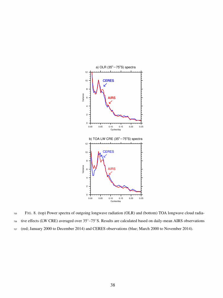
FIG. 8. (top) Power spectra of outgoing longwave radiation (OLR) and (bottom) TOA longwave cloud radia-
tive effects (LW CRE) averaged over 35◦–75◦S. Results are calculated based on daily-mean AIRS observations
(red; January 2000 to December 2014) and CERES observations (blue; March 2000 to November 2014).
725
726
727
38

Fig. A1. Comparing the cloud vertical structures associated with the four annular modes in CloudSAT obser-
vations and ERA-Interim reanalysis. Results in the left panels are reproduced from the shading in the bottom
panels of Figs. 1 and 3. Results in the middle and right panels show the corresponding regressions based on
daily-mean, zonal-mean cloud fractional cover from ERA-Interim based on the period 2007–2010 and 1979–
2011, respectively. ERA-Interim results are masked out poleward of 82◦ (the latitudinal limit of the CloudSAT
data). The thick black line indicates the height of the climatological-mean tropopause and zonally averaged
surface elevation over Antarctica. Black stippling indicates results that exceed the 95% confidence level based
on a two-tailed test of the t statistic, with the effective degrees of freedom computed as per Bretherton et al.
(1999, equation (31)).
728
729
730
731
732
733
734
735
73639

Fig. A2. Horizontal distribution of the regressions of pentad-mean cloud incidence (top) averaged between 7–
12 km for the SAM and NAM, (middle) averaged between 1.5–7 km for the SAM and NAM, (bottom) averaged
between 6–12 km for the SBAM and NABAM. Black stippling indicates results that exceed the 95% confidence
level based on a two-tailed test of the t statistic, with the effective degrees of freedom computed as per Bretherton
et al. (1999, equation (31)). The results have been smoothed with a National Center for Atmospheric Research
Command Language built-in 9-point smoothing function for the purpose of display only.
737
738
739
740
741
742
40
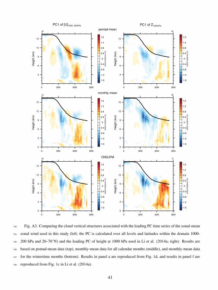
Fig. A3. Comparing the cloud vertical structures associated with the leading PC time series of the zonal-mean
zonal wind used in this study (left; the PC is calculated over all levels and latitudes within the domain 1000-
200 hPa and 20–70◦N) and the leading PC of height at 1000 hPa used in Li et al. (2014a; right). Results are
based on pentad-mean data (top), monthly-mean data for all calendar months (middle), and monthly-mean data
for the wintertime months (bottom). Results in panel a are reproduced from Fig. 1d, and results in panel f are
reproduced from Fig. 1c in Li et al. (2014a).
743
744
745
746
747
748
41