1 models of dark energy - centre for theoretical physics · 1 models of dark energy m. sami ......

1 Models of Dark Energy

M. Sami

Center for Theoretical Physics, Jamia Millia Islamia, New Delhi [email protected]

Summary. In this talk we present a pedagogical review of scalar field dynamics.The main emphasis is put on the underlying basic features rather than on con-crete scalar field models. Cosmological dynamics of standard scalar fields, phan-toms and tachyon fields is developed in detail. Scaling solutions are discussed em-phasizing their importance in modelling dark energy. The developed concepts areimplemented in an example of quintessential inflation. A brief discussion of scalingsolutions for coupled quintessence is also included.

Accelerated expansion seems to have played an important role in thedynamical history of our universe. There is a firm belief, at present, thatuniverse has passed through inflationary phase at early times and there havebeen growing evidences that it is accelerating at present. The recent measure-ment of the Wilkinson Microwave Anisotropy Probe (WMAP) in the CosmicMicrowave Background (CMB) made it clear that (i) the current state ofthe universe is very close to a critical and that (ii) primordial density per-turbations that seeded large-scale structure in the universe are nearly scale-invariant and Gaussian, which are consistent with the inflationary paradigm.As for the current accelerating of universe, it is supported by observations ofhigh redshift type Ia supernovae treated as standardized candles and, moreindirectly, by observations of the cosmic microwave background and galaxyclustering. The criticality of universe supported by CMB observations fixesthe total energy budget of universe. The study of large scale structure revealsthat nearly 30 percent of the total cosmic budget is contributed by dark mat-ter. Then there is a deficit of almost 70 percent; the supernovae observationstell us that the missing component is an exotic form of energy with largenegative pressure dubbed dark energy[1, 2, 3, 4]. The recent observations onbaryon oscillations provides yet another independent support to dark energyhypothesis. The idea that universe is in the state of acceleration is slowlyestablishing in modern cosmology.

The dynamics of our universe is described by Einstein equations in whichthe contribution of energy content of universe is represented by energy mo-mentum tensor appearing on RHS of these equations. The LHS representspure geometry given by the curvature of space time. Einstein equations intheir original form with energy momentum tensor of normal matter can notlead to acceleration. There are then two ways to obtain accelerated expansion,

2 M. Sami

either by supplementing energy momentum tensor by dark energy componentor by modifying the geometry itself. In the frame work of Dvali-Gabadadze-Porrati (DGP) brane worlds[5], the extra dimensional effects can lead to latetime acceleration. The other alternative which is largely motivated by phe-nomenological considerations is related to the introduction of inverse powersof Ricci scalar in the Einstein Hilbert action[6]. The third intriguing possi-bility is provided by Bekenstein relativistic theory of modified gravity[7, 8, 9]which apart from spin two field contains a vector and a scalar field.

Due to the simplicity of the mechanism, most of the work in cosmologyrelated late time acceleration is attributed to the assumption that within theframework of general relativity, cosmic acceleration is sourced by an energy-momentum tensor which has a large negative pressure. The simplest candi-date of dark, yet most difficult from field theoretic point of view, is providedby cosmological constant. Due to its non evolving nature it is plagued withfine tuning problem which can be alleviate in dynamically evolving scalarfield models. A variety of scalar field models have been conjectured for thispurpose including quintessence [10, 11], phantoms[12, 13, 14], K-essence [15]and recently tachyonic scalar fields[16]. In this talk we present a review ofcosmological dynamics of quintessence, phantoms and rolling tachyons. Wedescribe in detail the concepts of field dynamics relevant to cosmic evolutionwith a special emphasis on scaling solutions. The example of quintessentialinflation is worked out in detail.

We employ the metric signature (-,+,+,+) and use the reduced Planckmass M−2

p = 8πG ≡ κ2. In certain places we have adopted the unit Mp = 1.Finally we should mention that our list of references is restricted, in most ofthe places, we referred to reviews to help the readers.

1.1 Glimpses of FRW cosmology

The Freidmann-Robertson-Walker (FRW) model is based on the assumptionof homogeneity and isotropy which is approximately true at very large scales.The small deviation from homogeneity at early epochs played very importantrole in the dynamical history of our universe. The small density perturbationsare believed to have grown via gravitational instability into the structure wesee today in the universe. the origin of primordial perturbations is quan-tum mechanical and is out side the scope of standard big bang model. Inwhat follows we shall review main features of FRW model necessary for thesubsequent sections.

Homogeneity and isotropy forces the metric of space time to assume theform[17]

ds2 = −dt2 + a2(t)

(dr2

1 − kr2+ r2(dθ2 + sin2 θdφ2)

),

k = 0,±1 , (1.1)

1 Models of Dark Energy 3

where a(t) is cosmic scale factor. Coordinates r, θ and φ are known as comov-

ing coordinates. A freely moving particle comes to rest in these coordinates.Eq.(1.1) is purely a kinematic statement. In this problem the dynamics is

associated with the scale factor− a(t). Einstein equations allow to determinethe scale factor provided the matter content of universe is specified. Constantk occurring in the metric (1.1) describes the geometry of spatial section ofspace-time. Its value is also determined once the matter distribution in theuniverse is known. Observations have repeatedly confirmed the spatially flatgeometry (k = 0) in confirmation of the prediction of inflationary scenario.

1.1.1 Evolution equations

The differential equations for the scale factor and the matter density followfrom Einstein equations

Gµν ≡ Rµ

ν − 1

2δµν R = 8πGT µ

ν , (1.2)

whereGµ,ν is the Einstein tensor, Rµν is the Ricci tensor which depends onthe metric and its derivatives and R is Ricci scalar. The energy momentumtensor Tµν assumes a simplified form reminiscent of ideal perfect fluid in FRWbackground

Tµν = Diag (−ρ, p, p, p) . (1.3)

In this case the components of Gµν can easily be computed

G00 = − 3

a2

(a2 + k

)(1.4)

Gji =

1

a2

(2aa + a2 + k

)(1.5)

and all the other components of Einstein tensor are identically zero. Equations(1.2) then give the two independent equations

H2 ≡ a2

a2=

8πGρ

3− k

a2(1.6)

a

a= −4πG

3(ρ + 3p) . (1.7)

The energy momentum tensor is conserved by virtue of the Bianchi identity∆νGµ

ν = 0 leading to the continuity equation

ρ + 3H(ρ + p) = 0 . (1.8)

Equations (1.6), (1.7) & (1.8) make a redundant set of equations convenientto use; one of the two equations (1.7) & (1.8) can be obtained using the otherone and the Hubble equation (1.6). These equations supplemented with the

4 M. Sami

equation of state p(t) = p(ρ) uniquely determine a(t), p(t) and ρ(t). Constantk also gets determined

k

a2= H2 (Ω(t) − 1) , (1.9)

where Ω = ρ/ρc is the dimensionless density parameter and ρc = 3H2/8πGis critical density. The matter distribution clearly determines the spatial ge-ometry of our universe namely

Ω < 1 or ρ < ρc → k = −1 (1.10)

Ω = 1 or ρ = ρc → k = 0 (1.11)

Ω > 1 or ρ > ρc → k = 1 . (1.12)

In case of k = 0, the value the scale factor at the present epoch a0 canbe normalized to a convenient value, say, a0 = 1. In other cases it shouldbe determined using the observed values of H0 and Ω(0) from the relation

a0H0 =(|Ω(0) − 1|

)−1/2. Observations on cosmic micro wave background

radiation support the critical universe which is one of the predictions of in-flation. We would therefore assume k = 0 in the subsequent description.

• Acceleration

We now turn to the nature of expansion which is determined by the mat-ter content in the universe. Eq.(1.7) should be contrasted to the analogoussituation in Newtonian gravity

R = −4π

3GρR (1.13)

where R denotes the distance of the test particle from the center of a ho-mogeneous sphere of mass density ρ. In general theory of relativity (GR),unlike the Newtonian case, pressure contributes to energy density and mayqualitatively modify the dynamics. Indeed, from Eq.(1.7) we have

a > 0 if p < −ρ

3(1.14)

a < 0 if p > −ρ

3. (1.15)

Accelerated expansion, thus, is fuelled by an exotic form of matter of largenegative pressure dubbed dark energy which turns gravity into a repulsiveforce. The simplest example of a perfect fluid of negative pressure is providedby cosmological constant associated with ρ = constant. In this case thecontinuity equation (1.8) yields the relation p = −ρ. A host of scalar fieldsystems can also mimic negative pressure.

Assuming that the universe is filled with perfect barotropic fluid withconstant equation of state parameter w = p/ρ yields

ρ ∝ a−3(1+w) (1.16)

a(t) ∝ t2

3(1+w) (w > −1) (1.17)

a(t) ∝ eH t (w = −1) . (1.18)


The last equation corresponds to cosmological constant which can be addedto the energy momentum tensor of the perfect fluid. Interestingly, in fourdimension and at the classical level, the only modification Einstein equationsallow is associated with Tµν → +Tµν +Λgµν . Historically such a modificationwas first proposed by Einstein to achieve a static solution which turns outto be unstable. It was later dropped by him after the Hubble’s discovery. Inpresence of Λ, the evolution equations modify to

H2 =8πG

3+

Λ

3, (1.19)

a

a= −4πG

3(ρ + 3p) +

Λ

3. (1.20)

From Eq.(1.20), it clearly follows that Λ term contributes negatively to thepressure term and hence exhibits repulsive effect.

• Age crisis and cosmological constant

Apart from the dark energy problem, cosmological constant has other im-portant implications, in particular, in relation to the age problem. In anycosmological model with normal form of matter, the age of universe fallsshort as compared to the age of some well known old objects found in theuniverse. Remarkably, the presence of Λ can resolve the age problem. In orderto appreciate the problem, let us first consider the case of flat dust dominateduniverse (Ωm = 1)

a(t) ∝ t2/3 → H0 =2

3t0. (1.21)

The present value of the Hubble parameter H0 is not accurately know by theobservations

H−10 = h−10.98 × 1010years , (1.22)

0.8 < h < 0.64 → to = (8 − 10) × 109years. (1.23)

This model is certainly in trouble as its prediction for age of universe failsto meet the solar age constraint − t0 > (11 − 12) × 109years. One could try

to improve the situation by invoking the open model with Ω(0)m < 1. In this

case the age of universe is expected to be larger than the flat dust dominatedmodel− for less amount of matter, it would take longer for gravitationalinteraction to slow down the expansion rate to its present value. Indeed, inthis case we have the exact expression

H0t0 =1

1 − Ω(0)m

− Ω(0)m

2(1 − Ω(0)m )3/2

cosh−1

(2 − Ω

(0)m

Ω(0)m

)(1.24)

from which follows that

H0t0 = 1 , for Ω(0)m → 0 , (1.25)

H0t0 =2

3, for Ω(0)

m → 1 . (1.26)

6 M. Sami

For obvious reasons, in case of the closed universe, the age would even besmaller than 2/3H−1

0 . Though the age of universe is larger than 2/3H−10 for

vanishingly small value of Ω(0)m , such a model is note viable as Ω

(0)m ' 0.3 and

universe is critical to a good accuracy. The problem can be solved in a flatuniverse dominated by cosmological constant. In fact, in a flat universe with

two components (Ω(0)m + Ω

(0)Λ = 1), the Hubble equation

(a

a

)2

= H20

[Ω(0)

m

(a0

a

)2

+ Ω(0)Λ

](1.27)

has the solution

a

a0=

(Ω

(0)m

Ω(0)Λ

)1/3

sinh2/3

(3

2Ω(0)

m

1/2H0t

), (1.28)

which at t = t0 yields the following expression for the age of universe

t0 =2

3

H−10

Ω(0)Λ

1/2ln

1 + Ω

(0)Λ

1/2

Ω(0)m

1/2

. (1.29)

In Fig.1.1, we have plotted the age t0 versus Ωm. The age of universe islarger than H−1

0 for a Λ dominated universe. The numerical value of t0 (t0 '0.96H−1

0 ) is comfortable with observations for popular values of Ω(0)m = 0.3

and Ω(0)Λ = 0.7.

• Super acceleration

So far, we have restricted our attention to fluids with equation’ of stateparameter w ≥ −1. The case of w < −1 corresponds to phantom dark energy

and requires separate considerations. The power law expansion a(t) ∼ tn(n =2/3(1 + w)) corresponds to shrinking universe for n < 0 (w < −1). Thesituation can easily be remedied by changing the sign of t and by introducingthe origin of time ts

a(t) = (ts − t)n , (1.30)

which is the generic solution of evolution equations for super-negative valuesof w and it gives rise to a very different future course of evolution

H =n

ts − t(1.31)

R = 6

[a

a+

(a

a

)2]

= 6n(n − 1) + n2

(ts − t)2. (1.32)

The Hubble expansion rate diverges as t → ts corresponding to infinitelylarge energy density after a finite time in future. The curvature also grows toinfinity as t → ts. Such a situation is referred to Big Rip singularity. Big Rip


0.6

0.8

1

1.2

1.4

1.6

1.8

2

0 0.2 0.4 0.6 0.8 1

m(0)

Ω(0)m

t 0H

0

Ω + Ω =1Λ

OpenUniverse

Fig. 1.1. Age of universe (in the units of H−10 ) is plotted against Ω

(0)m in a flat

model (red line) with Ω(0)m + Ω

(0)Λ = 1 and matter dominated model (green line)

with Ω(0)m = 1.

can be avoided in specific models of phantom field with variable equation ofstate. It should also be emphasized that quantum effects become importantin a situation when curvature becomes large. In that case one should takeinto account the higher order curvature corrections to Einstein Hilbert actionwhich crucially modifies the structure of singularity.

1.1.2 Scalar fields− as perfect fluids in FRW background

Scalar fields naturally arise in unified models of interactions and also in stringtheory. Since the invent of inflation, they continue play an important role incosmology. They are frequently used as candidates of dark energy. In therecent years a variety of scalar field models namely quintessence, phantoms,tachyons, K-essence, dilatonic ghosts and others have been investigated in theliterature. In what follows we briefly describe some of these systems. Theirdynamics will be dealt with in detail in section III.

• Standard scalar field

Let us consider the scalar field minimally coupled to gravity

S = −∫ (

1

2gµν∂µφ∂νφ + V (φ)

)√−gd4x . (1.33)

The Euler Lagrangian equation

8 M. Sami

∂µ δ(√−gL)

δ∂µφ− δ(

√−gL)

δφ= 0 , (1.34)

√−g = a3(t)

for the action (1.33) in case of a homogeneous field acquires the form

φ + 3Hφ + Vφ = 0 , (1.35)

which is equivalent to the conservation equation

ρ

ρ+ 3H(1 + w) = 0 . (1.36)

The energy momentum tensor

Tµν = −21√−g

δS

δgµν(1.37)

for the field φ which arises from the action (1.33) is given by

Tµν = ∂µφ∂νφ − gµν

[1

2gµν∂µφ∂νφ + V (φ)

]. (1.38)

In the homogeneous and isotropic universe, the field energy density ρφ andpressure pφ obtained from Tµν are

T00 ≡ ρ =φ2

2+ V (φ), T i

i ≡ p =φ2

2− V (φ) . (1.39)

The field evolution equation(1.35) formally integrates to

ρ = ρ0e−6

∫ (1− 2V

φ2+2V

)daa . (1.40)

Thus the scaling of field energy density crucially depends upon the ratio ofkinetic to potential energy. Depending upon the scalar field regime ρ canmimic a behavior ranging from cosmological constant to stiff matter

ρ ∼ a−m 0 < m < 6 . (1.41)

This behavior is also clear intuitively namely the field φ rolling slowly alongthe flat wing of the potential gives rise to p ' −ρ where as it gives p ' ρwhile dropping fast along the steep part of the potential. Interestingly, onecan obtain the similar picture in the oscillatory regime for a power law typeof potential.

• Acceleration during oscillations.As the scalar field evolves towards the minimum of its, the slow role ceasesand a the scalar field enters into the regime of quasi periodic evolution with


decaying amplitude. In what follows , we shall assume that the potential iseven and has minimum at φ = 0 . When the field initially being displaced fromthe minimum of the potential, rolls below its slow roll value, the coherenceoscillation regime, ν >> H, commences. The evolution equation can thenbe approximately solved by separating the two times scales namely the fastoscillation time scale and the longer expansion time scale. On the first timescale, the Hubble expansion can be neglected, and one obtain φ as a functionof time;

t − t0 = ±∫

1√2(Vm − V (φ))

dφ , (1.42)

where ρ ≡ Vm ≡ V (φm); Vm being the maximum current value of the po-tential energy and φm being the field amplitude . On the longer time scale ρand φm slowly decrease because Hubble damping term in equation ( 1 ). Theaverage adiabatic index γ is defined as

γ =

⟨ρ + p

ρ

⟩=

⟨φ2

ρ

⟩, (1.43)

where< . > denotes the time average over one oscillation . Equation (4) thentells that expansion during oscillations would continue (a > 0) if γ < 2

3 . Theadiabatic evolution of a(t) and ρ is given by ,

a(t) ∝ t23γ , (1.44)

ρ ≡ V (φm) ∝ t−2 . (1.45)

As φ = −dVdφ , the condition γ < 2

3 can equivalently be written

γ =

⟨φ2

ρ

⟩=

< φV,φ >

Vm= 2(1 − < V >

Vm) ,

= 2

∫ φm

0(1 − V (φ)/Vm)

12 dφ

∫ φm

0(1 − V (φ)/Vm)−

12 dφ

=2p

p + 1, (1.46)

for a power law potential V ∼ φ2p, which gives the average value of theequation of state parameter

〈w〉 =p − 1

p + 1, p < 1/2 → acceleration . (1.47)

Thus a quadratic potential, on the average, mimics dust where as the quarticpotential exhibits radiation like behavior. It is really interesting that thescalar field in oscillatory regime can give rise to dark energy for p < 1/2.

While developing scalar fields models of dark energy, it is important tohave some control on its dynamics. In what follows we show how to constructa field potential viable to desired cosmic evolution.

10 M. Sami

• Construction of field potential for a given cosmological evolu-

tion

After the invent of cosmological inflation, scalar field models have been fre-quently used in cosmology in various contexts; they play a central role spe-cially in modelling dark energy. Our focus in the review will also be aroundthese models. We should, however, caution the reader that the scalar fieldmodels have limited predictive power. The merits of these models shouldtherefore be judged on the basis of generic features that might emerge inthem. Indeed, for a priori given cosmological evolution, we can always con-struct a field potential that would produce it. We shall illustrate this simplefact in case of a power law expansion for a general cosmological backgroundgoverned by the Friedmann equation

H2 =ρq

A, (1.48)

where q = 2, 2/3 correspond to Randall-Sundrum (RS) and Gauss-Bonnet(GB) brane worlds respectively; A is a constant which takes different valuesin different patches. We show below how to construct the field potential forordinary scalar field propagating in a general background described by (1.48).

φ + 3Hφ +dV

dφ. (1.49)

Using Eqs. (1.36) and (1.48) we obtain

1 + w = −(

2

3q

)H

H2. (1.50)

From evolution equation (1.49) and the expression φ2 = V (1 + w)(1−w)−1,we have the differential equation for the field potential V

V

V= − f + 6Hf

1 + f, (1.51)

where f = (1 + w)(1 − w)−1. Integrating (1.51) respecting (1.50), we get

V (t) =C

3q

(3qH2 + H

H2(q−1)/q

), (1.52)

where C = A1/q is an integrating constant. Expressing f in terms of H andits derivative through equation (1.50) and using (1.51), we obtain the φ(t)

φ(t) =

(2C

3q

)1/2 ∫ [− H

H2(q−1)/q

]1/2

dt . (1.53)


Equations (refpoteq) and (1.53) allow to find the field potential with a givenexpansion dynamics prescribed by a(t). For a(t) ∼ tn, we are interested, wehave

φ − φ0 = Dnqt(q−1)/q , (1.54)

V (t) = Cn2/q

(1 − n−(q+2)/2q

3q

)t−2/q , (1.55)

where Dnq = n(2−q)/q(2C/3q)1/2(q/q − 1) and q 6= 1. Combining (1.54) and(1.55) we get the expression for the potential as function of φ

V (φ) = V0φ−(2/q−1) . (1.56)

In case q = 1, the field logarithmically depends on time t and Eq. (1.56) leadsto the well known exponential potential. For q = 2 corresponding to RS, weobtain V (φ) ∼ 1/φ2. The case of high energy GB regime (q = 2/3) leads tothe power law behavior of V (φ)

V (φ) = V0φ6 . (1.57)

• Phantom Field.All these models of scalar field lead to the equation of state parameter wgreater than or equal to minus one. However, the recent observations do notseem to exclude values of this parameter less than minus one. It is thereforeimportant to look for theoretical possibilities to describe dark energy withw < −1 called phantom energy. In our opinion, the simplest alternative isprovided by a phantom field, scalar field with negative kinetic energy. Such afield can be motivated from S-brane constructs in string theory. Historically,phantom fields were first introduced in Hoyle’s version of the Steady StateTheory. In adherence to the Perfect Cosmological Principle, a creation field(C-field) was for the first time introduced [12] to reconcile with homogeneousdensity by creation of new matter in the voids caused by the expansion ofUniverse. It was further refined and reformulated in the Hoyle and Narlikartheory of gravitation [13]. Though the quantum theory of phantom fields isproblematic, it is nevertheless interesting to examine the cosmological conse-quences of these fields at the classical level.

The Lagrangian of the phantom field minimally coupled to gravity is givenby

L = (16πG)−1R +1

2gµν∂φµ∂φν − V (φ) , (1.58)

where V (φ) is the phantom potential. The kinetic energy term of the phantomfield in (1.58) enters with the opposite sign in contrast to the ordinary scalarfield (we remind the reader that we use the metric signature, -,+,+,+). Ina spatially flat FRW cosmology, the stress tensor that follows from (1.58)acquires the diagonal form T α

β = diag (−ρ, p, p, p) where the pressure andenergy density of field φ are given by

12 M. Sami

ρ = − φ2

2+ V (φ), p = − φ2

2− V (φ) . (1.59)

The corresponding equation of state parameter is now given by

w ≡ p

ρ=

φ2

2 + V (φ)

φ2

2 − V (φ). (1.60)

For ρ > 0, w < −1.The equations of motion which follow from (1.58) are

H =1

2M2p

φ2 (1.61)

H2 =1

3M2p

ρφ (1.62)

φ + 3Hφ = V ′(φ) . (1.63)

Note that the evolution equation (1.63) for the phantom field is same as thatof the normal scalar field with inverted potential allowing the field with zeroinitial kinetic energy to roll up the hill; i.e., from lower value of potential tohigher one. At the first look such a situation looks pathological. However, atpresent, the situation in cosmology is remarkably tolerant to any pathologyif it can lead to a viable model.

As mentioned above the equation of state parameter with super negativevalues leads to Big Rip which can be avoided in a particular class of models.For instance, let us consider consider a model with

V (φ) = V0

[cosh

(αφ

Mp

)]−1

. (1.64)

Due to its peculiar properties, the phantom field, released at a distance fromthe origin with zero kinetic energy, moves to wards the top of the potentialand crosses over to the other side and turns ba ck to execute the dampedoscillation about the maximum of the potential (see Fig.1.2). After a certainperiod of ti me the motion ceases and the field settles on the top of thepotential permanently to mimic the de-Sitter like behavior (w = −1).

• Rolling tachyon

It was recently suggested that rolling tachyon condensate, in a class of stringtheories, might have interesting cosmological consequences. It was shown bySen[16] that the decay of D-branes produces a pressure-less gas with finiteenergy density that resembles classical dust. Rolling tachyon has an interest-ing equation of state whose parameter smoothly interpolates between −1 and0. Attempts have been made to construct viable cosmological model usingrolling tachyon field as a suitable candidate for inflaton, dark matter or dark


0

0.1

0.2

0.3

0.4

0.5

0.6

0.7

0.8

0.9

1

-6 -4 -2 0 2 4 6

φ/ΜP

VV0

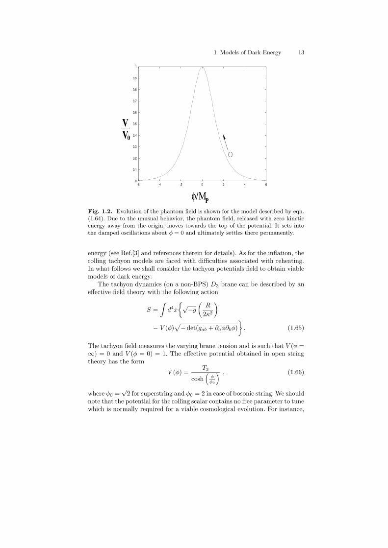
Fig. 1.2. Evolution of the phantom field is shown for the model described by eqn.(1.64). Due to the unusual behavior, the phantom field, released with zero kineticenergy away from the origin, moves towards the top of the potential. It sets intothe damped oscillations about φ = 0 and ultimately settles there permanently.

energy (see Ref.[3] and references therein for details). As for the inflation, therolling tachyon models are faced with difficulties associated with reheating.In what follows we shall consider the tachyon potentials field to obtain viablemodels of dark energy.

The tachyon dynamics (on a non-BPS) D3 brane can be described by aneffective field theory with the following action

S =

∫d4x

√−g

(R

2κ2

)

− V (φ)√−det(gab + ∂aφ∂bφ)

. (1.65)

The tachyon field measures the varying brane tension and is such that V (φ =∞) = 0 and V (φ = 0) = 1. The effective potential obtained in open stringtheory has the form

V (φ) =T3

cosh(

φφ0

) , (1.66)

where φ0 =√

2 for superstring and φ0 = 2 in case of bosonic string. We shouldnote that the potential for the rolling scalar contains no free parameter to tunewhich is normally required for a viable cosmological evolution. For instance,

14 M. Sami

the late time evolution of the scalar field with potential (1.66) can mimicthe current accelerated expansion of universe provided the brane tension T3

could be tuned to the critical energy density at the current epoch. However,this is absolutely out of scope from viewpoint of string theory as it leads tovery small masses for massive string states. We are, therefore, led to thinkof another mechanism which would affect the D-brane tension and the slopeof the scalar field potential without touching the string length and the stringcoupling constant. We shall hereafter show that these features are shared bythe warped compactification. Consider the following warped metric

ds210 = β(yi)gabdxadxb + β−1(yi)gijdyidyj , (1.67)

where the coordinates yi represent the compact dimensions, and gij representmetric in the compact space. At some point in the y-space the factor β canbe small. This corresponds to a scenario in which the brane moves in thecompact dimensions reducing its tension. The tachyon action at a point y inthe y-space becomes

S = −∫

d4xβ2V (φ)√

−det(gab + β−1∂aφ∂bφ) .

(1.68)

Normalizing the scalar field as φ →√

βφ, one finds the standard Dirac-Born-Infeld (DBI) type action

S = −∫

d4xV (φ)√

−det(gab + ∂aφ∂bφ) , (1.69)

where now the potential is

V (φ) =V0

cosh(√

βφφ0

) , with V0 = β2T3 . (1.70)

The constant V0 can be less than T3 for small values of β with β < 1. Insections to follow, we shall also consider other forms of tachyon potentialwhich can be inspired by string theory and others which are introduced bypurely phenomenological considerations.

In a spatially flat Friedmann-Robertson-Walker (FRW) background, Theenergy density ρ and the pressure p which follow from action (1.65) are givenby,

ρ =V (φ)√1 − φ2

, (1.71)

p = −V (φ)

√1 − φ2 . (1.72)

The equation of motion of the rolling scalar field follows from Eq. (??)


φ

1 − φ2+ 3Hφ +

Vφ

V (φ)= 0 , (1.73)

which is equivalent to the conservation equation

ρ

ρ+ 3H(1 + w) = 0 . (1.74)

The tachyon dynamics is very different from the standard field case. Irrespec-tive of steepness of tachyon potential, its equation of state parameter variesbetween 0 and −1. Thus reheating is impossible to achieve in this model, iftachyon field is to be an inflaton. However, it can be used as a candidate ofdark energy as shown in one of the following sections.

We now look for the potential which can lead to power law type of expan-sion in case of tachyon field. In this case, the expression for (1 + w) is alsogiven by the Eq. (1.50) but the equation of state parameter w has a simplerelation with φ

φ2 = 1 + w . (1.75)

Using (1.50) and (1.75) we get

φ(t) =

∫ [− 2H

3qH2

]dt . (1.76)

From Eqs. (1.48), (1.50) and (1.72) we can express the potential V (t) as

V (t) = (−w)1/2ρ = H2/qA1/q

(1 +

2

3q

H

H2

). (1.77)

In case of Born-Infeld scalar field, Eqs. (1.76) and (1.77) determine the fieldφ(t) and the potential V (t) for given scale factor a(t). In case of power lawexpansion a(t) ∝ tn, we obtain from (1.76) and (1.77)

φ(t) − φ0 =

(2

3nq

)1/2

t , (1.78)

V (t) = n2/qA1/q

(1 − 2

3nq

)1/2

t−2/q , (1.79)

which finally lead toV (φ) = V0φ

−2/q . (1.80)

We should note that the power law expansion in the present case takes placewith the constant velocity of the the field (see Eq. (1.78)) which is typicalof Born-Infeld dynamics. For q = 1 corresponding to standard GR, (1.80)reduces to inverse square potential earlier obtained by Padmanabhan[18]. Incase of RS which corresponds to q = 2, we get V (φ) ∼ 1/φ. In case of high

16 M. Sami

energy GB regime (= 2/3), the potential which can implement power lawexpansion turns out to be

V (φ) =V0

φ3. (1.81)

This sort of hierarchy of potentials is understandable; in GR the requiredpotential behaves as 1/φ2 whereas in RS scenario due to the extra branedamping, the power law expansion can be achieved with the less inversepower of field . In the high energy GB regime, the Hubble damping is weakerthan the standard FRW cosmology, thereby requiring larger inverse power ofthe field.

1.1.3 Current acceleration and observations in brief

The direct evidence of current acceleration of universe is related to the ob-servation of luminosity distance of high redshift supernovae by two groupsindependently in 1998[1, 2]. The luminosity distance at high redshift is largerin dark energy dominated universe. Thus supernovae would appear fainterin case the universe is dominated by dark energy. The luminosity distancecan be used to estimate the apparent magnitude m of the source given itsabsolute magnitude M . using the following relation often used in astronomy

m − M = 5 log

(DL

Mpc

)+ 25 . (1.82)

In order to get a feeling of the phenomenon (the reader is referred to excellentreview of Perivolaropoulos[19] for details) let us consider two supernovae1997ap at redshift z = 0.83 with m = 24.32 and 1992P at z = 0.026 withapparent magnitude M = 16.08. Since the supernovae are supposed to bethe standard candles, their absolute magnitude is same. Secondly we shalluse the fact that DL(z) ' z/H0 for small value of z. Eq.(1.82) then yieldsthe following estimate

H0DL ' 1.16 (1.83)

The theoretical estimate for the luminosity distance for flat universe tells us

DL ' 0.95H−10 , Ω(0)

m = 1 , (1.84)

DL ' 1.23H−10 , Ω(0)

m = 0.3, Ω(0)Λ = 0.7 . (1.85)

The above estimate clearly lands a strong support to the case of dark energydominated universe (see Ref.[19] for details).

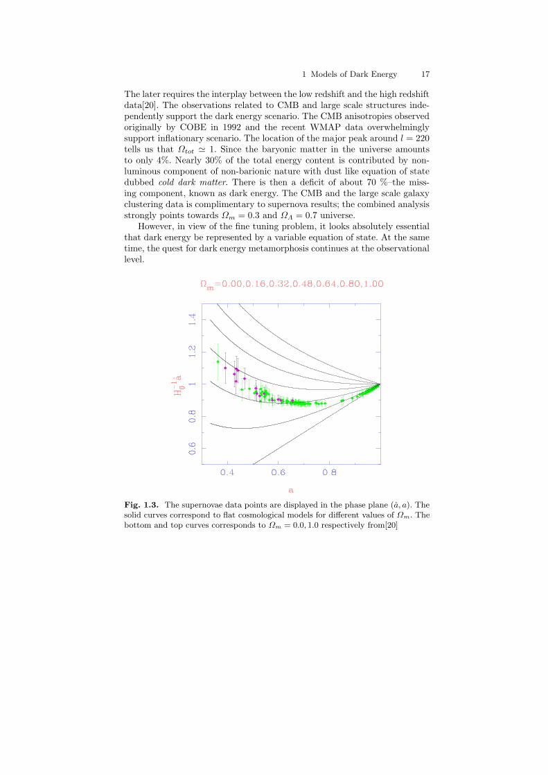
An interesting proposal for visualizing acceleration in supernovae datawas proposed in Ref.[20]. The authors displayed the data with error bars onthe phase plane (a, a), see Fig.1.3 for flat models with different values of Ωm.The data at low red shift clearly confirms the presence of accelerated phasebut due to large error bars it is not possible to choose a particular model.


The later requires the interplay between the low redshift and the high redshiftdata[20]. The observations related to CMB and large scale structures inde-pendently support the dark energy scenario. The CMB anisotropies observedoriginally by COBE in 1992 and the recent WMAP data overwhelminglysupport inflationary scenario. The location of the major peak around l = 220tells us that Ωtot ' 1. Since the baryonic matter in the universe amountsto only 4%. Nearly 30% of the total energy content is contributed by non-luminous component of non-barionic nature with dust like equation of statedubbed cold dark matter. There is then a deficit of about 70 %–the miss-ing component, known as dark energy. The CMB and the large scale galaxyclustering data is complimentary to supernova results; the combined analysisstrongly points towards Ωm = 0.3 and ΩΛ = 0.7 universe.

However, in view of the fine tuning problem, it looks absolutely essentialthat dark energy be represented by a variable equation of state. At the sametime, the quest for dark energy metamorphosis continues at the observationallevel.

Fig. 1.3. The supernovae data points are displayed in the phase plane (a, a). Thesolid curves correspond to flat cosmological models for different values of Ωm. Thebottom and top curves corresponds to Ωm = 0.0, 1.0 respectively from[20]

18 M. Sami

1.2 Cosmological constant Λ

Historically Λ was introduced by Einstein to achieve a static solution whichturned out to be unstable. However, after the Hubble’s redshift discoveryin 1929, the motivation for having Λ was lost and it was dropped. Sincethen the cosmological constant was introduced time and again to remove thediscrepancies between theory and observations and withdrawn when thesediscrepancies were resolved. It had come and gone several times making itscome back finally, seemingly for ever!, in 1998 through supernova Ia observa-tions. Recently much efforts have gone in understanding Λ in the frame workof quantum fields and string theory. In what follows we shall briefly mentionthese issues.

• Λ as a natural free parameter of classical gravity

It should be noted that a term proportional to the the metric gµν ismissing on the right hand side of Einstein equations (1.2). Indeed the Bianchidentity ∆νGµ

ν = 0 implies that

Gµν = +κTµν − Λgµν , (1.86)

with∇νTµν = 0 , (1.87)

where Tµν is a symmetric tensor, and κ and Λ are constants. The demandthat it should in the first approximation reduce to the Newtonian equationfor gravitation will require Tµν to represent the energy momentum tensorfor matter and κ = 8πG/c2 with Λ being negligible at the stellar scale. TheEinstein equations should then read as

Gµν ≡ Rµν − 1

2gµνR = 8πGTµν − Λgµν . (1.88)

Note that the constant Λ enters into the equation naturally. It was intro-duced by Einstein in an ad-hoc manner to have a physically acceptable staticmodel of the Universe and was subsequently withdrawn when Friedmannfound the non-static model with acceptable physical properties. We wouldhowever like to maintain that it appears in the equation as naturally as thestress tensor Tµν and hence should be considered on the same footing[21]. Asfor the classical physics, the cosmological constant is a free parameter of thetheory and its numerical value should be determined from observations.

• Λ arising due to vacuum fluctuations.Cosmological constant can be associated with vacuum fluctuations in the

quantum field theoretic context. Though the arguments are still at the levelof numerology but may have far reaching consequences. Unlike the classicaltheory the cosmological constant Λ in this scheme is no longer a free pa-rameter of the theory. Broadly the line of thinking takes the following route.


The quantum effects in GR become important when the Einstein Hilbert ac-tion becomes of the order of Planck’s constant; this happens at the Planck’slength Lp =

√(8πG) ∼ 10−32cm corresponding to Planck energy which is

of the order of M4p ∼ 1072GeV 4. In the language of field theory, a system is

described by a set of quantum fields. The ground state energy dubbed zeropoint energy or vacuum energy of a free quantum field is infinite.

This contribution is related the ordering ambiguity of fields in the classi-cal Lagrangian and disappears when normal ordering is adopted. Since thisprocedure of throwing out the vacuum energy is ad hoc, one might try tocancel it by introducing the counter terms. The later, however requires finetuning and may be regarded as unsatisfactory. Whether or not the zero pointenergy in field theory is realistic is still a debatable question. The divergenceis related to the modes of very small wave length. As we are ignorant ofphysics around Planck scale we might be tempted to introduce a cut off atLp and associate Λ with this fundamental scale. Thus we arrive at an esti-

mate of vacuum energy ρv ∼ M4p (corresponding mass scale− MV ∼ (ρ

1/4V )

which is away by 120 orders of magnitudes from the observed value of thisquantity. The vacuum energy may not be felt in the laboratory but playsimportant role in GR through its contribution to the energy momentum ten-sor as < Tµν >0= −ρV gµν and appears on the right hand side of Einsteinequations

Rµν − 1

2gµνR = 8πG (Tµν+ < Tµν >0) . (1.89)

The problem of zero point energy is naturally resolved by invoking super-symmetry which has many other remarkable features. In the supersymmetricdescription, every bosonic degree of freedom has its Fermi counter part whichcontributes zero point energy with opposite sign compared to the bosonic de-gree of freedom thereby doing away with the vacuum energy. It is in thissense the supersymmetric theories do not admit a non-zero cosmological con-stant. However, we know that we do not leave in supersymmetric vacuumstate and hence it should be broken. For a viable supersymmetric scenario,for instance if it is to be relevant to hierarchy problem, the suppersymmetrybreaking scale should be around Msusy ∼ 103GeV . We are still away fromthe observed value by many orders of magnitudes. At present we do not knowhow Planck scale or SUSY breaking scales is related to the observed vacuumscale.

• Λ from string theory− de-Sitter vacuua a la KKLT

In view of the observations related to supernova, large scale clustering andMicro wave background, the idea of late time acceleration has reached thelevel of general acceptability. It is, therefore, not surprising that tremendousefforts have recently been made in finding out de-Sitter solutions in super-gravity and string theory. Using flux compactification, Kachru, Kallosh, Lindeand Trivedi (KKLT) formulated a procedure to construct de-Sitter vacua oftype IIB string theory[22]. They demonstrated that the life time of the vacua

20 M. Sami

is larger that the age of universe and hence these solutions can be consideredas stable for practical purposes. Although a fine-tuning problem of Λ stillremains in this scenario, it is interesting that string theory gives rise to astable de-Sitter vacua with all moduli fixed. We note that a vast number ofdifferent choices of fluxes leads to a complicated landscape with more than10100 vacua. We should believe, if we can, that we live in one of them!. .

1.2.1 Fine tuning problem

Inspite of the fact that introduction of Λ does not require an adhoc assump-tion and it is also not ruled out by observation as a candidate of dark energy;the scenario base upon Λ is faced with the worst type of fine tuning problem.The numerical value of Λ at early epochs should be tuned to a fantastic accu-racy so as not to disturb todays physics. In order to appreciate the problem,let us consider the following ratio

ρΛ

3H2(t)8πG

= ΩΛ

(H0

H(t)

)2

, (1.90)

where ΩΛ = (ρΛ/ρc) ' 0.7. It will not disturb our estimate if we assumeradiation domination today. In that case the ratio H/H0 scales as a−2 andsince the temperature is inversely proportional to the scale factor a, we find

ρΛ

3H2(t)8πG

= 0.7

(T0

T

)4

. (1.91)

Since at the Planck (T = Tp = Mp ) epoch T0/T ' 10−31, the ratio ofρΛ to 3H2/8πG turns out to be of the order of 10−123. On the theoreticalground, such a fine tuning related to the scale of cosmological constant isnot acceptable. This problem led to the investigation of scalar field modelsof dark energy which can alleviate this problem to a considerable extent.

1.3 Dynamically evolving scalar field models of dark

energy

Before entering into the detailed investigations of field dynamics, we shallfirst examine some of the general constraints on scalar field Lagrangian if itis to be relevant to cosmology.

1.3.1 Broad features of scalar field dynamics and cosmological

relevance of scaling solutions

The scalar field aiming to describe dark energy is often imagined to be a relicof early universe physics. Depending upon the model, the scalar field energy


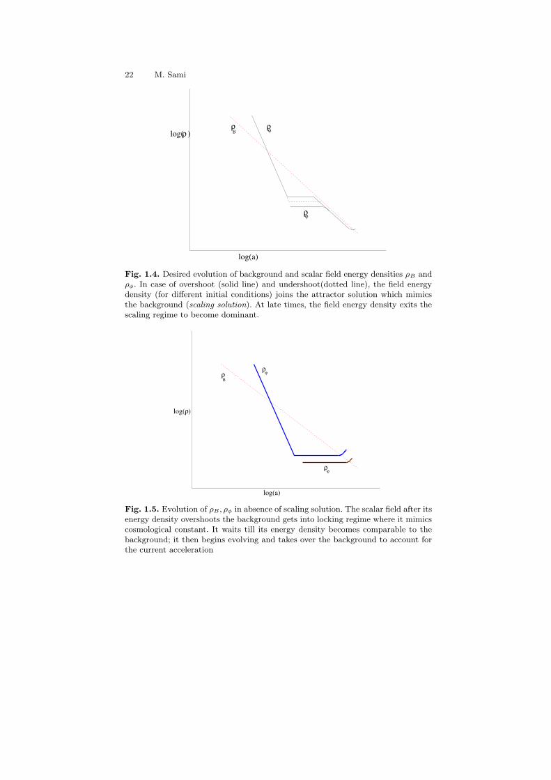
density may be larger or smaller than the background (radiation/matter) en-ergy density ρB . In case it is larger than the back ground density, the densityρφ should scale faster than ρB allowing radiation domination to commencewhich requires a steep scalar field potential. In this case the field energy den-sity overshoots the background and becomes sub dominant to it. This leadsto the locking regime for the scalar field. The field unlocks the moment itsenergy density becomes comparable to the background. Its further course ofevolution crucially depend upon the form of field potential. In order to obtainviable dark energy models, we require that the energy density of the scalarfield remains unimportant during radiation and matter dominant eras andemerges only at late times to give rise to the current acceleration of universe.It is then important to investigate cosmological scenarios in which the en-ergy density of the scalar field mimics the background energy density. Thecosmological solutions which satisfy this condition is called scaling solutions

[23]. Namely scaling solutions are characterised by the relation

ρB/ρφ = const . (1.92)

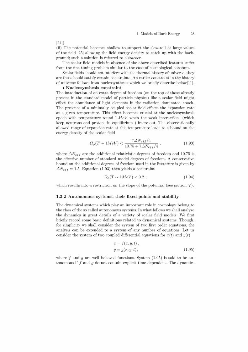
We shall shortly demonstrate that exponential potentials give rise to scal-ing solutions for a minimally coupled scalar field, allowing the field energydensity to mimic the background being sub-dominant during radiation andmatter dominant eras. In this case, for any generic initial conditions, the fieldwould sooner or later enter into the scaling regime (see Fig.1.4). This allowsto alleviate the fine tuning problem to a considerable extent. The same thingis true in case of the undershoot, i.e., when the field energy is smaller ascompared to the background. In Fig.1.5, we have displayed a cartoon depict-ing the field dynamics in absence of scaling solutions. For instance, we shallsee later, scaling solutions , which could mimic realistic background, do notexist in case of phantom and tachyon fields. These models are plagued withadditional fine tuning problem.

Scaling solutions exist in case of a steep exponential potential V (φ) ∼exp(λφ/Mp) with λ2 > 3(1 + wm) ( the field dominated case correspondsto λ2 < 3(1 + wm) whereas λ2 < 2 gives rise to ever accelerating universe).Nucleosynthesis puts stringent restriction on any additional degree of freedomwhich translates into a constraint on the slope of the exponential potentialλ.

• Late time evolution and exit from scaling regime

Obviously, scaling solution is non-accelerating as the equation of state of thefield φ equals to that of the background fluid (wφ = wm) in this case. Onethen requires to introduce a late time feature in the potential allowing to exitfrom the scaling regime. Broadly there are two ways to get the required latetime behavior for a minimally coupled scalar field:(i) The potential changes into a power law type V ∼ φ2q which gives latetime acceleration for q < 1/2 (e.g., V (φ) = V0 [cosh(αφ/Mp) − 1]

q, q > 0

22 M. Sami

log(a)

log( )ρρB

ρ

ρ

ϕ

ϕ

Fig. 1.4. Desired evolution of background and scalar field energy densities ρB andρφ. In case of overshoot (solid line) and undershoot(dotted line), the field energydensity (for different initial conditions) joins the attractor solution which mimicsthe background (scaling solution). At late times, the field energy density exits thescaling regime to become dominant.

log(a)

ρ

ρB

ρϕ

ρϕ

log( )

Fig. 1.5. Evolution of ρB , ρφ in absence of scaling solution. The scalar field after itsenergy density overshoots the background gets into locking regime where it mimicscosmological constant. It waits till its energy density becomes comparable to thebackground; it then begins evolving and takes over the background to account forthe current acceleration


[24]).(ii) The potential becomes shallow to support the slow-roll at large valuesof the field [25] allowing the field energy density to catch up with the back-ground; such a solution is referred to a tracker.

The scalar field models in absence of the above described features sufferfrom the fine tuning problem similar to the case of cosmological constant.

Scalar fields should not interfere with the thermal history of universe, theyare thus should satisfy certain constraints. An earlier constraint in the historyof universe follows from nucleosynthesis which we briefly describe below[11].

• Nucleosynthesis constraint

The introduction of an extra degree of freedom (on the top of those alreadypresent in the standard model of particle physics) like a scalar field mighteffect the abundance of light elements in the radiation dominated epoch.The presence of a minimally coupled scalar field effects the expansion rateat a given temperature. This effect becomes crucial at the nucleosynthesisepoch with temperature round 1MeV when the weak interactions (whichkeep neutrons and protons in equilibrium ) freeze-out. The observationallyallowed range of expansion rate at this temperature leads to a bound on theenergy density of the scalar field

Ωφ(T ∼ 1MeV ) <7∆Neff/4

10.75 + 7∆Neff/4, (1.93)

where ∆Neff are the additional relativistic degrees of freedom and 10.75 isthe effective number of standard model degrees of freedom. A conservativebound on the additional degrees of freedom used in the literature is given by∆Neff ' 1.5. Equation (1.93) then yields a constraint

Ωφ(T ∼ 1MeV ) < 0.2 , (1.94)

which results into a restriction on the slope of the potential (see section V).

1.3.2 Autonomous systems, their fixed points and stability

The dynamical systems which play an important role in cosmology belong tothe class of the so called autonomous systems. In what follows we shall analyzethe dynamics in great details of a variety of scalar field models. We firstbriefly record some basic definitions related to dynamical systems. Though,for simplicity we shall consider the system of two first order equations, theanalysis can be extended to a system of any number of equations. Let usconsider the system of two coupled differential equations for x(t) and y(t)

x = f(x, y, t) ,

y = g(x, y, t) , (1.95)

where f and g are well behaved functions. System (1.95) is said to be au-tonomous if f and g do not contain explicit time dependent. The dynamics

24 M. Sami

of these systems can be analysed in a standard way.• Fixed or critical pointsA point (xc, yc) is said to be a fixed point or critical point of the autonomoussystem if and only if

(f, g)|xc,yc= 0 (1.96)

and a critical point (xc, yc) is called an attractor in case

(x(t), y(t)) → (xc, yc) for t → ∞ . (1.97)

• Stability around the fixed pointsThe stability of each point can be studied by considering small perturbationsδx and δy around the critical point (xc, yc), i.e.,

x = xc + δx , y = yc + δy . (1.98)

Substituting into Eqs. (1.104) and (1.105), leads to the first-order differentialequations:

d

dN

(δxδy

)= M

(δxδy

), (1.99)

where matrix M depends upon xc and yc

M =

(∂f∂x

∂f∂y

∂g∂x

∂g∂y

)

(x=xc,y=yc)

The general solution for the evolution of linear perturbations can be writ-ten as

δx = C1exp(µ1N) + C2exp(µ2N) , (1.100)

δy = C3exp(µ1N) + C4expp(µ2N) , (1.101)

where µ1 and µ2 are the eigenvalues of matrix M. Thus the stability aroundthe fixed points depends upon the nature of eigenvalues. One generally usesthe following classification:

– (i) Stable node: µ1 < 0 and µ2 < 0.– (ii) Unstable node: µ1 > 0 and µ2 > 0.– (iii) Saddle point: µ1 < 0 and µ2 > 0 (or µ1 > 0 and µ2 < 0).– (iv) Stable spiral: The determinant of the matrix M is negative and the

real parts of µ1 and µ2 are negative.

1.3.3 Quintessence

Let us consider a minimally coupled scalar field φ with a potential V (φ):

L =1

2εφ2 + V (φ) , (1.102)


where ε = +1 for an ordinary scalar field. Here we allow the possibility ofphantom (ε = −1) as we see in the next subsection.

In what follows we shall consider a cosmological evolution when the uni-verse is filled by a scalar field φ and a barotropic fluid with an equation ofstate wm = pm/ρm. We introduce the following dimensionless quantities:

x ≡ κφ√6H

, y ≡ κ√

V√3H

, λ ≡ − Vφ

κV, Γ =

V Vφφ

V 2φ

. (1.103)

For the Lagrangian density (1.102) the Einstein equations can be written inthe following autonomous form (see Ref.[3] for details) :

dx

dN= −3x +

√6

2ελy2

+3

2x[(1 − wm)εx2 + (1 + wm)(1 − y2)

], (1.104)

dy

dN= −

√6

2λxy

+3

2y[(1 − wm)εx2 + (1 + wm)(1 − y2)

], (1.105)

dλ

dN= −

√6λ2(Γ − 1)x , (1.106)

together with a constraint equation

εx2 + y2 +κ2ρm

3H2= 1 , (1.107)

where N ≡ log (a). We note that the equation of state w and the fraction ofthe energy density Ωφ for the field φ is

wφ ≡ p

ρ=

εx2 − y2

εx2 + y2, Ωφ ≡ κ2ρ

3H2= εx2 + y2 . (1.108)

We also define the total effective equation of state:

weff ≡ p + pm

ρ + ρm= wm + (1 − wm)εx2 − (1 + wm)y2 . (1.109)

An accelerated expansion occurs for weff < −1/3. In this subsection we shallconsider the normal scalar field (ε = +1).

Constant λ

From Eq. (1.103) we find that the constant λ corresponds to an exponentialpotential [23]:

V (φ) = V0e−κλφ . (1.110)

26 M. Sami

Name x y Range Stability Ωφ γφ

(a) 0 0 ∀λ, γ s. p. for 0 < γ < 2 0 –

(b1) 1 0 ∀λ,γ un. n. for λ <√

6 1 2

s p for λ >√

6

(b2) -1 0 ∀λ, γ un. n. for λ > −√

6 1 2

s. p. for λ < −√

6

(c) λ/√

6 [1 − λ2/6]1/2 λ2 < 6 st. n. for λ2 < 3γ 1 λ2/3st. n. for 3γ < λ2 < 6

(d) (3/2)1/2 γ/λ [3(2 − γ)γ/2λ2]1/2 λ2 > 3γ st. n. for 3γ < λ2 3γ/λ2 γ< 24γ2/(9γ − 2)st. sp. for λ2 >24γ2/(9γ − 2)

Table 1.1. The properties of the critical points (s=saddle, p=point, un=unstable,n=node, st=stable, sp=spiral) from Ref.[3]. Here γ is defined by γ ≡ 1 + wm.

In this case Eq. (1.106) is dropped from the dynamical system. One canobtain the fixed points by setting dx/dN = 0 and dy/dN = 0 in Eqs. (1.104)and (1.105). This is summarized in Table I.

In the next section we shall extend our analysis to the more general casein which dark energy is coupled to dark matter. The readers may refer tothe next section in order to know precise values of the eigenvalues in a moregeneral system. From TABLE I we find that there exists two stable fixedpoints (c) and (d). The point (c) is a stable node for λ2 < 3γ. Since theeffective equation of state is weff = wφ = −1+λ2/3, the accelerated expansionoccurs for λ2 < 2 in this case. The point (d) corresponds to a scaling solutionin which the energy density of the field φ decreases proportionally to that ofthe barotropic fluid (γφ = γ). Although this fixed point is stable for λ2 > 3γ,we do not have an accelerated expansion in the case of non relativistic darkmatter.

The above analysis of the critical points shows that one can obtain anaccelerated expansion provided that the solutions approach the fixed point(c) with λ2 < 2, in which case the final state of the universe is the scalar-fielddominated one (Ωφ = 1). The scaling solution (d) is not viable to explain thelate-time acceleration. However this can be used to provide the cosmologicalevolution in which the scalar field decreases proportionally to that of thematter or radiation. If the slope of the exponential potential becomes shallowto satisfy λ2 < 2 near to the present, the universe exits from the scaling regimeand approaches the fixed point (c) giving rise to an accelerated expansion.

Dynamically changing λ

Exponential potentials correspond to constant λ and Γ = 1. Let us considerthe potential V (φ) along which the field rolls down toward plus infinity (φ →


∞) This means that x > 0 in Eq. (1.106). If the condition

Γ > 1 , (1.111)

is satisfied, λ decreases toward 0. Hence the slope of the potential becomes flatas λ → 0, thereby giving rise to an accelerated expansion at late times. Thecondition (1.111) is regarded as the tracking condition under which the energydensity of φ eventually catches up that of the fluid. In order to constructviable quintessence models, we require that the potential should satisfy thecondition (1.111). For example, one has Γ = (n + 1)/n > 1 for the inversepower-law potential V (φ) = V0φ

−n with n > 0. This means that the trackingoccurs for this potential.

When Γ < 1 the quantity λ increases toward infinity. Since the potentialis steep in this case, the energy density of the scalar field becomes negligiblecompared to that of the fluid. Hence we do not have an accelerated expansionat late times

In order to obtain the dynamical evolution of the system we need to solveEq. (1.106) together with Eqs. (1.104) and (1.105). Although λ is dynami-cally changing, one can exploit the discussion of constant λ by considering“instantaneous” critical points.

1.3.4 Phantoms

The phantom field corresponds to a negative kinematic sign, i.e, ε = −1 inEq. (1.102). Let us consider the exponential potential given by Eq. (1.110).In this case Eq. (1.106) is dropped from the dynamical system. In Table 1.2we show fixed points for the phantom field. The only stable solution is thescalar-field dominant solution (b), in which case the equation of the field φ is

wφ = −1 − λ2/3 . (1.112)

Hence wφ is less than −1. The scaling solution (c) is unstable and exists onlyfor wm < −1. We note that the effective equation of state of the universeequals to wφ, i.e., weff = −1 − λ2/3. In this case the Hubble rate evolves as

H =2

3(1 + weff)(t − ts), (1.113)

where ts is an integration constant. Hence H diverges for t → ts. This isso-called the Big Rip singularity at which the Hubble rate and the energydensity of the universe exhibit divergence. We note that the phantom fieldrolls up the potential hill in order to lead to the increase of the energy density.

When the potential of the phantom is different from the exponential type,the quantity λ is dynamically changing in time. In this case the point (b)in Table 1.2 can be regarded as an instantaneous critical point. Then theequation of state wφ varies in time, but the field behaves as a phantom sincewφ = −1 − λ2/3 < −1 is satisfied.

28 M. Sami

Name x y Range Stab. Ωφ wφ

(a) 0 0 No for 0 ≤ Ωφ ≤ 1 s. p. 0 –

(b) −λ/√

6 [1 + λ2/6]1/2 All values st. n. 1 −1 − λ2/3

(c)√

6(1+wm)2λ

[−3(1−w2

m)

2λ2 ]1/2 wm < −1 s. p. −3(1+wm)

λ2 wm

Table 1.2. The properties of the critical points (s=saddle, p=point, n=node,st=stable) for ε = −1 (from[3]).

1.3.5 Tachyons

We shall take into account the contribution of a barotropic perfect fluid withan equation of state pB = (γ − 1)ρB . Then the background equations ofmotion are for rolling tachyon system are

H = − φ2V (φ)

2M2p

√1 − φ2

− γ

2

ρB

M2p

, (1.114)

φ

1 − φ2+ 3Hφ +

Vφ

V= 0 , (1.115)

ρB + 3γHρB = 0 , (1.116)

together with a constraint equation:

3M2p H2 =

V (φ)√1 − φ2

+ ρB . (1.117)

Defining the following dimensionless quantities:

x = φ , y =

√V (φ)√

3HMp

, (1.118)

we obtain the following autonomous equations

dx

dN= −(1 − x2)(3x −

√3λy) , (1.119)

dy

dN=

y

2

(−√

3λxy − 3(γ − x2)y2

√1 − x2

+ 3γ

), (1.120)

dλ

dN= −

√3λ2xy(Γ − 3/2) . (1.121)

where

λ = −MpVφ

V 3/2, Γ =

V Vφφ

V 2φ

. (1.122)


We note that the allowed range of x and y is 0 ≤ x2 + y4 ≤ 1 from therequirement: 0 ≤ Ωφ ≤ 1. Hence both x and y are finite in the range 0 ≤x2 ≤ 1 and 0 ≤ y ≤ 1. The effective equation of state for the field φ is

γφ =ρφ + pφ

ρφ= φ2 , (1.123)

which means that γφ ≥ 0. The condition for inflation corresponds to φ2 < 2/3.

Constant λ

From Eq. (1.121) we find that λ is a constant for Γ = 3/2. This case corre-sponds to an inverse square potential (For details, see Ref. [3])

V (φ) = M2φ−2 . (1.124)

The scalar-field dominated solution (Ωφ = 1), in this case, correspondsto γφ = λ2/3 which can lead to an accelerated expansion for λ2 < 2. Noscaling solution which could mimic radiation or matter exist in this case (seeRef.[3]). Since λ is given by λ = 2Mp/M , the condition for an acceleratedexpansion gives a super-Planckian value of the mass scale, i.e., M >

√2Mp.

Such a large mass is problematic since this shows the breakdown of classicalgravity. This problem can be alleviated for the inverse power-law potentialV (φ) = M4−nφ−n, as we will see below.

Dynamically changing λ

When the potential is different from the inverse square potential given inEq. (1.124), λ is a dynamically changing quantity. As we have seen in thesubsection of quintessence, there are basically two cases: (i) λ evolves towardzero, or (ii) |λ| increases toward infinity. The case (i) is regarded as thetracking solution in which the energy density of the scalar field eventuallydominates over that of the fluid. This situation is realized when the potentialsatisfies the condition

Γ > 3/2 , (1.125)

as can be seen from Eq. (1.121). The case (ii) corresponds to the case inwhich the energy density of the scalar field becomes negligible compared tothe fluid.

As an example let us consider the inverse power-law potential given by

V (φ) = M4−nφ−n , n > 0 . (1.126)

In this case one has Γ = (n + 1)/n. Hence the scalar-field energy densitydominates at late times for n < 2.

30 M. Sami

x y Ωφ weff

−√

6Q3(1−wm)

0 2Q2

3(1−wm)1

1 0 1 1

−1 0 1 1λ√

6[(1 − λ2

6)]1/2 1 −1 + λ2

3√

6(1+wm)2(λ+Q)

[2Q(λ+Q)+3 (1−w2

m)

2(λ+Q)2]1/2 Q(λ+Q)+3 (1+wm)

(λ+Q)2λwm−Q(λ+Q)

Table 1.3. Q 6= 0, from[3]

There exist a number of potentials that exhibit the behavior |λ| → ∞asymptotically. For example V (φ) = M 4−nφ−n with n > 2 and V (φ) =V0e

−µφ with µ > 0. In the latter case one has Γ = 1. In these cases, pressureless dust ia late time attractor where as the accelerated expansion can occuras a transient phenomenon. Extra fine tuning is needed in this case to obtainthe current acceleration.

1.4 Scaling solutions in models of coupled quintessence

As we have already seen in the previous section, exponential potentials giverise to scaling solutions for a minimally coupled scalar field, allowing thefield energy density to mimic the background being sub-dominant duringradiation and matter dominant eras. In the previous section we found outthe expression for Ωφ for scaling solution which after combining with thenucleosynthesis constraint (1.94) gives

Ωφ ≡ ρφ

ρφ + ρm=

(1 + wm)

λ2< 0.2 → λ > 5 . (1.127)

In this case, however, one can not have an accelerated expansion at latetimes since ρφ mimics background. We briefly mentioned as how to exit thescaling regime, in models of minimally coupled scalar fields, to account forthe current acceleration of universe.

If the scalar field φ is coupled to the background fluid, it is possibleto obtain an accelerated expansion at late-times even in the case of steepexponential potentials. In this section we implement the coupling Q betweenthe field and the barotropic fluid and show that scaling solutions can alsoaccount for accelerated expansion. The evolution equations in presence ofcoupling acquire the form

ρφ + 3H(1 + wφ)ρφ = −Qρmφ (1.128)

ρm + 3H(1 + wm)ρm = Qρmφ , (1.129)

H = −1

2

[(1 + wm)ρφ + (1 + wm)ρm

]. (1.130)


H2 =ρφ + ρm

3, (1.131)

where coupling Q is field dependent in general. For simplicity, we shall as-sume constant coupling. The autonomous form of equations for exponentialpotential in presence of coupling takes the following form

dx

dN= −3x +

√6

2λy2 +

3

2x[(1 − wm)εx2 + (1.132)

(1 + wm)(1 − c1y2)]−

√6Q

2(1 − x2 − y2) ,

dy

dN= −

√6

2λxy +

3

2y[(1 − wm)x2 + (1 + wm)(1 − y2)

]. (1.133)

We display the critical points for coupled quintessence in the table in whichthe last entry corresponds to scaling solution with effective equation of stateweff = 0 for Q = 0 consistent with earlier analysis. It is remarkable thatweff → −1 for Q >> λ. Thus scaling solutions can account for accelerationin presence of coupling between field and the barotropic fluid. Unfortunately,they are not acceptable from CMB constraints. The general investigations ofperturbations for coupled quintessence require further serious considerations.

1.5 Quintessential inflation

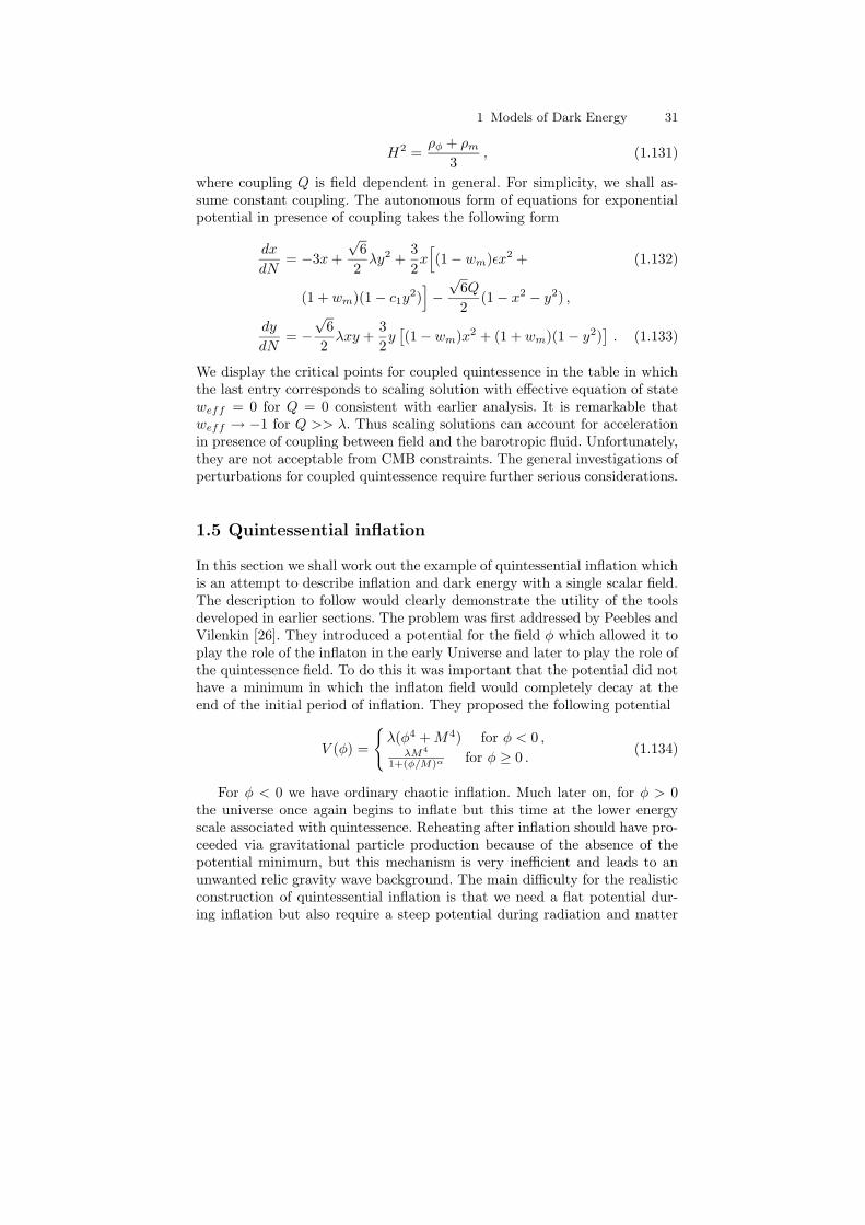
In this section we shall work out the example of quintessential inflation whichis an attempt to describe inflation and dark energy with a single scalar field.The description to follow would clearly demonstrate the utility of the toolsdeveloped in earlier sections. The problem was first addressed by Peebles andVilenkin [26]. They introduced a potential for the field φ which allowed it toplay the role of the inflaton in the early Universe and later to play the role ofthe quintessence field. To do this it was important that the potential did nothave a minimum in which the inflaton field would completely decay at theend of the initial period of inflation. They proposed the following potential

V (φ) =

λ(φ4 + M4) for φ < 0 ,

λM4

1+(φ/M)α for φ ≥ 0 .(1.134)

For φ < 0 we have ordinary chaotic inflation. Much later on, for φ > 0the universe once again begins to inflate but this time at the lower energyscale associated with quintessence. Reheating after inflation should have pro-ceeded via gravitational particle production because of the absence of thepotential minimum, but this mechanism is very inefficient and leads to anunwanted relic gravity wave background. The main difficulty for the realisticconstruction of quintessential inflation is that we need a flat potential dur-ing inflation but also require a steep potential during radiation and matter

32 M. Sami

dominated periods. There are some nice resolutions of quintessential inflationin braneworld scenarios as we shall see below (see review.[27] and referencestherein on this theme). In these models, the scalar field exhibits the proper-ties of tracker field. As a result it goes into hiding after the commencementof radiation domination; it emerges from the shadow only at late times toaccount for the observed accelerated expansion of universe. These modelsbelong to the category of non oscillating models in which the standard re-heating mechanism does not work. In this case, one can employ an alternativemechanism of reheating via quantum-mechanical particle production in timevarying gravitational field at the end of inflation. However, then the inflatonenergy density should red-shift faster than that of the produced particles sothat radiation domination could commence. And this requires a steep fieldpotential, which of course, cannot support inflation in the standard FRWcosmology. This is precisely where the brane[29] assisted inflation comes toour rescue. In the 4+1 dimensional brane scenario inspired by the Randall-Sundrum (RS) model, the standard Friedman equation is modified to

H2 =1

3M2p

ρ

(1 +

ρ

2λb

), (1.135)

The presence of the quadratic density term ρ2/λb (high energy correc-tions) in the Friedmann equation on the brane changes the expansion dy-namics at early epochs (see Ref[29] for details on the dynamics of braneworlds) Consequently, the field experiences greater damping and rolls downits potential slower than it would during the conventional inflation. This effectis reflected in the slow-roll parameters which have the form [29]

ε = εFRW1 + V/λb

(1 + V/2λb)2 ,

η = ηFRW (1 + V/2λb)−1

, (1.136)

where

εFRW =M2

p

2

(V ′

V

)2

, ηFRW = M2p

(V ′′

V

)(1.137)

are slow roll parameters in the absence of brane corrections. The influence ofthe brane term becomes important when V/λb 1 and in this case we get

ε ' 4εFRW(V/λb)−1, η ' 2ηFRW(V/λb)

−1. (1.138)

Clearly slow-roll (ε, η 1) is easier to achieve when V/λb 1 and on thisbasis one can expect inflation to occur even for relatively steep potentials,such the exponential and the inverse power-law. The model of quintessentialinflation [27] based upon reheating via gravitational particle production isfaced with difficulties associated with excessive production of gravity waves.


Indeed the reheating mechanism based upon this process is extremely inef-ficient. The energy density of so produced radiation sis typically one partin 1016 to the scalar-field energy density at the end of inflation. As a result,these models have prolonged kinetic regime during which the amplitude of pri-mordial gravity waves enhances and violates the nucleosynthesis constraint.Hence, it is necessary to look for alternative mechanisms more efficient thanthe gravitational particle production to address the problem. However thisproblem may be alleviated in instant preheating scenario [28] in the pres-ence of an interaction g2φ2χ2 between inflaton φ and another field χ. Thismechanism is quite efficient and robust, and is well suited to non-oscillatingmodels. It describes a new method of realizing quintessential inflation on thebrane in which inflation is followed by ‘instant preheating’. The larger reheat-ing temperature in this model results in a smaller amplitude of relic gravitywaves which is consistent with the nucleosynthesis bounds[27]. Fig.1.6 showsthe post inflationary evolution of scalar field energy density for the potentialgiven by

V (φ) = V0 [cosh(κλφ) − 1]n

. (1.139)

This potential has following asymptotic forms:

V (φ) '

V0e−nκλφ (|λφ| 1, φ < 0) ,

V0(κλφ)2n (|λφ| 1) ,(1.140)

where V0 = V0/2n. The existence of scaling solution for exponential potential

(V ∼ exp(κλφ)) tells us that λ2 > 3γ where as nucleosynthesis constraintmakes the potential further steeper as Ωφ = 3γ/λ2 < 0.2 → λ > 5. Po-tential (1.140) is suitable for unification of inflation and quintessence. In thiscase, for a given number of e-foldings, the COBE normalization allows toestimate the brane tension λb and the field potential at the end of inflation.Tuning the model parameters (λ − slope of the potential and V0), we can

account for the current acceleration with Ω(0)φ ' 0.7 and Ω

(0)m ' 0.3[27]. How-

ever, the recent measurement of CMB anisotropies by WMAP places fairlystrong constraints on inflationary models. The ratio of tensor perturbationsto scalar perturbations turns out to be large in case of steep exponentialpotential pushing the model outside the 2σ observational bound [30]. How-ever, the model can be rescued in case a Gauss-Bonnet term is present infive dimensional bulk [31, 32]. In order to see how it comes about, let usconsider Einstein-Gauss-Bonnet action for five dimensional bulk containinga 4D brane

S =1

2κ25

∫d5x

√−gR − 2Λ5 + αGB[R2 − 4RABRAB

+ RABCDRABCD]

+

∫d4x

√−h(Lm − λb) , (1.141)

34 M. Sami

-140

-120

-100

-80

-60

-40

-20

0

0 5 10 15 20 25

Log 1

0 ( ρ

/ M

p4 )

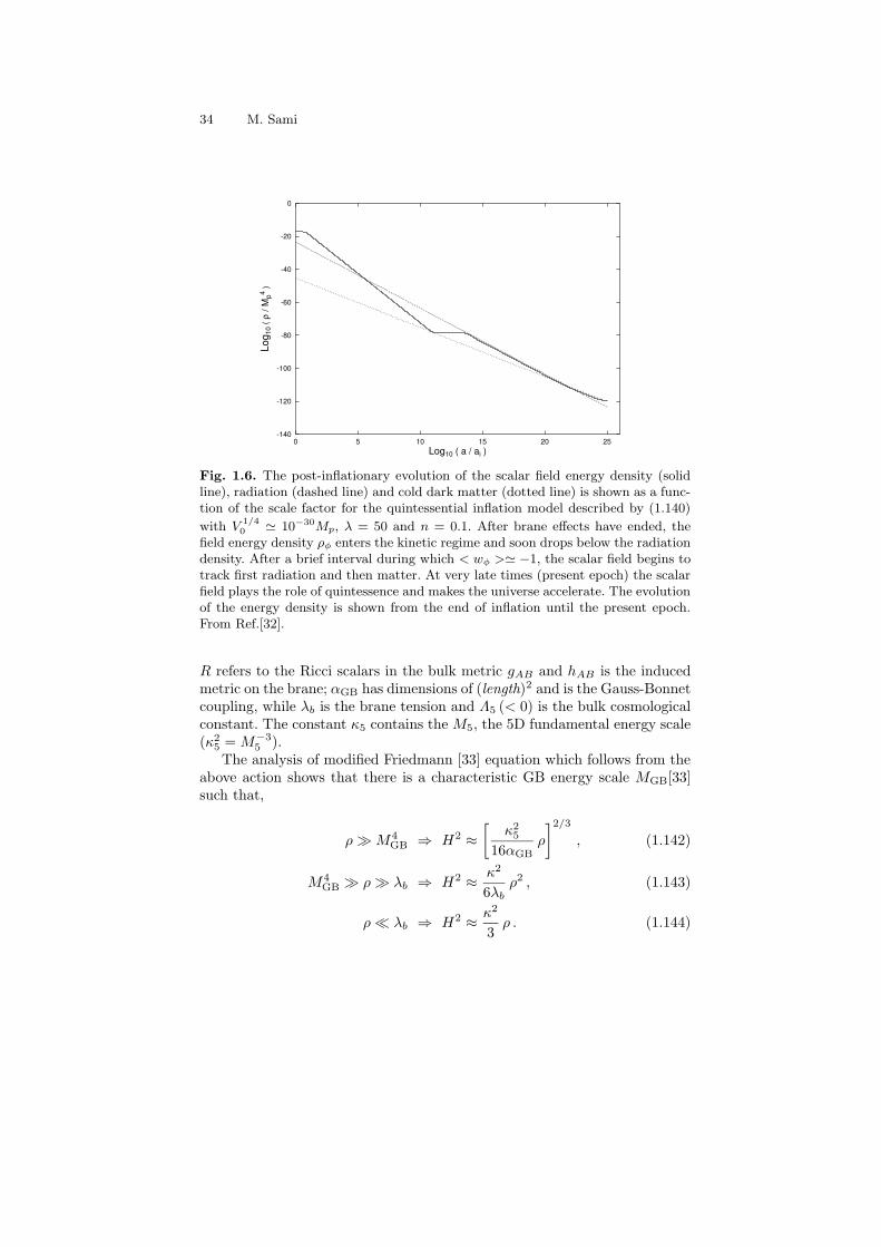
Log10 ( a / ai )

Fig. 1.6. The post-inflationary evolution of the scalar field energy density (solidline), radiation (dashed line) and cold dark matter (dotted line) is shown as a func-tion of the scale factor for the quintessential inflation model described by (1.140)

with V1/40 ' 10−30Mp, λ = 50 and n = 0.1. After brane effects have ended, the

field energy density ρφ enters the kinetic regime and soon drops below the radiationdensity. After a brief interval during which < wφ >' −1, the scalar field begins totrack first radiation and then matter. At very late times (present epoch) the scalarfield plays the role of quintessence and makes the universe accelerate. The evolutionof the energy density is shown from the end of inflation until the present epoch.From Ref.[32].

R refers to the Ricci scalars in the bulk metric gAB and hAB is the inducedmetric on the brane; αGB has dimensions of (length)2 and is the Gauss-Bonnetcoupling, while λb is the brane tension and Λ5 (< 0) is the bulk cosmologicalconstant. The constant κ5 contains the M5, the 5D fundamental energy scale(κ2

5 = M−35 ).

The analysis of modified Friedmann [33] equation which follows from theabove action shows that there is a characteristic GB energy scale MGB[33]such that,

ρ M4GB ⇒ H2 ≈

[κ2

5

16αGBρ

]2/3

, (1.142)

M4GB ρ λb ⇒ H2 ≈ κ2

6λbρ2 , (1.143)

ρ λb ⇒ H2 ≈ κ2

3ρ . (1.144)


It should be noted that Hubble law acquires an unusual form for energieshigher than the GB scale. Interestingly, for an exponential potential, themodified Eq.(1.142) leads to exactly scale invariant spectrum for primordialdensity perturbations. Inflation continues below GB scale and terminates inthe RS regime leading to the spectral index very close to one. However, asshown in Refs.[33, 31], the tensor to scalar ratio of perturbations(R) alsoincreases towards the high energy GB regime. It is known that the value of Ris larger in case of RS brane world as compared to the standard GR. Whilemoving from the RS regime characterized by H2 ∝ ρ2 to GB regime describedby H2 ∝ ρ2/3, we pass through an intermediate region which mimics GR likebehavior. It is not surprising that the ratio R has minimum at an intermediateenergy scale between RS and GB, see Fig.1.7. We conclude that a successfulscenario of quintessential inflation on the Gauss-Bonnet braneworld can beconstructed which agrees with CMB+LSS observations.

1.6 Conclusions

In this talk we have reviewed the general features of scalar field dynamics.Our discussion has been mainly pedagogical in nature. we tried to presentthe basic features of standard scalar field, phantoms and rolling tachyon.Introducing the basic definitions and concepts, we have shown as how to findthe critical pints and investigate stability around them. This is a standardtechnique needed for building the scalar field models desired for a viablecosmic evolution. The two often used mechanisms for the exit from scalingregime are also described in detail. In case of phantoms and rolling tachyon,we have shown that there exits no scaling solutions which would mimic therealistic background fluid (radiation/matter). Thus, in these case, there willbe dependency on the initial conditions of the field leading to fine tuningproblems. These models should therefore be judged on the basis of genericfeatures which might arise in them. The rolling tachyon is inspired by stringtheory whereas as phantoms might be supported by observations!.

After developing the basic techniques of scalar field dynamics, we workedout the example of quintessential inflation. we have shown in detail howto implement the techniques for building a unified model of inflation andquintessence with a single scalar field.

In this talk we have not touched upon the observational status of darkenergy models. We have also not discussed the alternatives to dark energy.The interested reader is refereed to other talks on these topics in the sameproceedings. The supernovae observations are not yet sufficient to decide themetamorphosis of dark energy. There have been claims and anti-claims fordynamically evolving dark energy using supernovae, CMB and large scalestudies. Given the present observational status of cosmology, it would be

36 M. Sami

ns

R

0.9 0.95 1 1.05 1.10

0.1

0.2

0.3

0.4

0.5

0.6

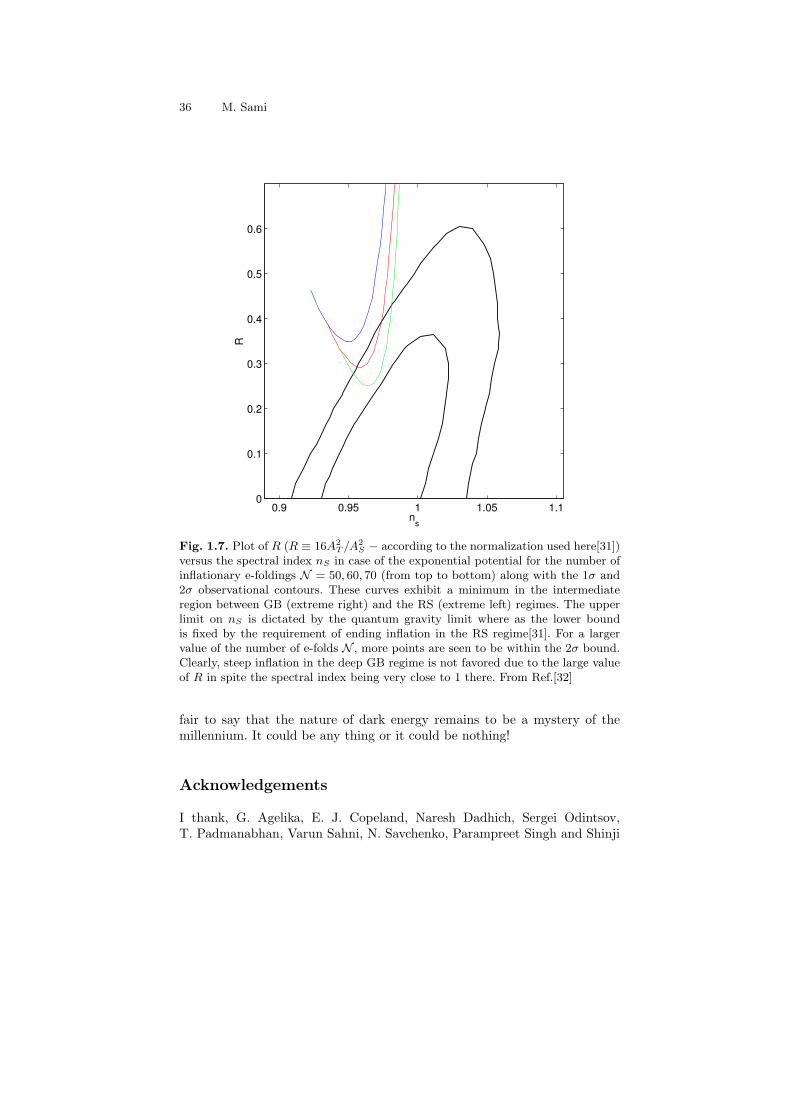
Fig. 1.7. Plot of R (R ≡ 16A2T /A2

S − according to the normalization used here[31])versus the spectral index nS in case of the exponential potential for the number ofinflationary e-foldings N = 50, 60, 70 (from top to bottom) along with the 1σ and2σ observational contours. These curves exhibit a minimum in the intermediateregion between GB (extreme right) and the RS (extreme left) regimes. The upperlimit on nS is dictated by the quantum gravity limit where as the lower boundis fixed by the requirement of ending inflation in the RS regime[31]. For a largervalue of the number of e-folds N , more points are seen to be within the 2σ bound.Clearly, steep inflation in the deep GB regime is not favored due to the large valueof R in spite the spectral index being very close to 1 there. From Ref.[32]

fair to say that the nature of dark energy remains to be a mystery of themillennium. It could be any thing or it could be nothing!

Acknowledgements

I thank, G. Agelika, E. J. Copeland, Naresh Dadhich, Sergei Odintsov,T. Padmanabhan, Varun Sahni, N. Savchenko, Parampreet Singh and Shinji


Tsujikawa for useful discussions. I also thank Gunma National College ofTechnology (Japan) for hospitality where the part of the talk was written. Iam extremely thankful to the organisers of Third Aegean Summer school forgiving me opportunity to present the review on dark energy models.

References

1. S. Perlmutter et al., 1999, Astrophys. J 517, 565.2. A. Riess, et al. 1999, Astrophys. J,117, 707.3. E. J. Copeland, M. Sami and Shinji Tsujikawa, Dynamics of dark energy, hep-

th/0603057.4. V. Sahni and A. A. Starobinsky, Int. J. Mod. Phys. D 9, 373 (2000); S. M. Car-

roll, Living Rev. Rel. 4, 1 (2001); T. Padmanabhan, Phys. Rept. 380, 235(2003); P. J. E. Peebles and B. Ratra, Rev. Mod. Phys. 75, 559 (2003).

5. Arthur Lue, astro-ph/0510068.6. S. Nojiri, S.D. Odintsov, hep-th/0601213.7. Jacob D. Bekenstein, Phys. Rev. D 70 (2004) 083509; Erratum-ibid. D71 (2005)

069901.8. Robert H. Sanders, astro-ph/0601431.9. Luz Maria Diaz-Rivera, Lado Samushia, B. Ratra, astro-ph/0601153.

10. C. Wetterich, Nucl. Phys. B 302, 668 (1988); J. A. Frieman, C. T. Hill, A. Steb-bins and I. Waga, Phys. Rev. Lett. 75, 2077 (1995) [arXiv:astro-ph/9505060];I. Zlatev, L. M. Wang and P. J. Steinhardt, Phys. Rev. Lett. 82, 896 (1999)[arXiv:astro-ph/9807002]; P. Brax and J. Martin, Phys. Rev. D 61, 103502(2000) [arXiv:astro-ph/9912046]; T. Barreiro, E. J. Copeland and N. J. Nunes,Phys. Rev. D 61, 127301 (2000) [arXiv:astro-ph/9910214]; A. Albrecht andC. Skordis.

11. P. G. Ferreira and M. Joyce, Phys. Rev. Lett. 79, 4740 (1997) [arXiv:astro-ph/9707286]

12. F. Hoyle, Mon. Not. R. Astr. Soc. 108, 372 (1948); 109, 365 (1949).13. F. Hoyle and J. V. Narlikar, Proc. Roy. Soc. A282, 191 (1964); Mon. Not. R.

Astr. Soc. 155, 305 (1972); J. V. Narlikar and T. Padmanabhan, Phys. Rev. D32, 1928 (1985).

14. R. R. Caldwell, Phys. Lett. B 545, 23-29 (2002).15. C. Armendariz-Picon, T. Damour, and V. Mukhanov, Phys. Lett. B458, 219

(1999), hep-th/9904075; J. Garriga and V. Mukhanov, Phys. Lett. B458, 219(1999), hep-th/9904176; T. Chiba, T. Okabe, and M. Yamaguchi, Phys. Rev.D62, 023511 (2000), astro-ph/9912463; C. Armendariz-Picon, V. Mukhanov,and P. J. Steinhardt, Phys. Rev. Lett. 85, 4438 (2000), astro-ph/0004134;C. Armendariz-Picon, V. Mukhanov, and P. J. Steinhardt, Phys. Rev. D63,103510 (2001), astro-ph/0006373; M. Malquarti and A. R. Liddle, Phys. Rev.D66, 023524 (2002), astro-ph/0203232

16. A. Sen, JHEP 0204, 048 (2002); JHEP 0207, 065 (2002); A. Sen, JHEP 9910,008 (1999); M. R. Garousi, Nucl. Phys. B584, 284 (2000); Nucl. Phys. B 647,117 (2002); JHEP 0305, 058 (2003); E. A. Bergshoeff, M. de Roo, T. C. deWit, E. Eyras, S. Panda, JHEP 0005, 009 (2000); J. Kluson, Phys. Rev. D 62,126003 (2000); D. Kutasov and V. Niarchos, Nucl. Phys. B 666, 56 (2003).

38 M. Sami

17. T. Padmanabhan, astro-ph/0602117.18. T. Padmanabhan, Phys.Rev. D 66 (2002) 021301.19. L. Perivolaropoulos, astro-ph/0601014.20. T. Padmanabhan and T. Roy Choudhury, Mon. Not. Roy. Astron.Soc.344

(2003) 823.21. N. Dadhich, gr-qc/0405115.22. Shamit Kachru, Renata Kallosh, Andrei Linde, Sandip P. Trivedi, Phys. Rev.

D 68 (2003) 046005.23. E. J. Copeland, A. R. Liddle and D. Wands, ”Phys. Rev. D 57, 4686 (1998).24. V. Sahni and L. M. Wang, Phys. Rev. D 62, 103517 (2000).25. T. Barreiro, E. J. Copeland and N. J. Nunes, Phys. Rev. D 61, 127301 (2000).26. P. J. E. Peebles and A. Vilenkin, Phys. Rev. D 59, 063505 (1999).27. M. Sami and N. Dadhich, hep-th/04050.28. G. N. Felder, L. Kofman and A. D. Linde, Phys. Rev. D 60, 103505 (1999);

G. N. Felder, L. Kofman and A. D. Linde, Phys. Rev. D 59, 123523 (1999).29. R. Maartens, Living Rev. Rel. 7, 7 (2004).30. A. R. Liddle and A. J. Smith, Phys. Rev. D 68, 061301 (2003); S. Tsujikawa

and A. R. Liddle, JCAP 0403, 001 (2004).31. S. Tsujikawa, M. Sami and R. Maartens, Phys. Rev. D 70, 063525 (2004).32. M. Sami and V. Sahni, Phys. Rev. D 70, 083513 (2004).33. J.-F. Dufaux, J. Lidsey, R. Maartens, M. Sami, hep-th/0404161.

1 models of dark energy - centre for theoretical physics · 1 models of dark energy m. sami ......

Documents