1 Lecture Notes - Production Functions - 1/5/2017 D.A.

2 Introduction

• Production functions are one of the most basic components of economics

• They are important in themselves, e.g.

—What is the level of returns to scale?

—How do input coeffi cients on capital and labor change over time?

—How does adoption of a new technology affect production?

—How much heterogeneity is there in measured productivity across firms, and what ex-plains it?

—How does the allocation of firm inputs relate to productivity

• Also can be important as inputs into other interesting questions, e.g. dynamic models ofindustry evolution, evaluation of firm conduct (e.g. collusion)

• For this lecture note, we will work with a simple two input Cobb-Douglas production function

Yi = eβ0Kβ1i L

β2i e

εi

where i indexes firms, Ki is units of capital, Li is units of labor, and Yi is units of output.(β0, β1, β2) are parameters and εi captures unobservables that affects output (e.g. weather,soil quality, management quality)

• Take natural logs to get:yi = β0 + β1ki + β2li + εi

• This can be extended to

—Additional inputs, e.g. R&D (knowledge capital), dummies representing discrete tech-nologies, different types of labor/capital, intermediate inputs.

— Later we will see more flexible models

yi = f (ki, li;β) + εi

yi = f (ki, li, εi;β) (with scalar/monotonic εi)

yi = β0 + β1iki + β2ili + εi

3 Endogeneity Issues

• Problem is that inputs ki, li are typically choice variables of the firm. Typically, these choicesare made to maximize profits, and hence will often depend on unobservables εi.

• Of course, this dependence depends on what the firm knows about εi when they make theseinput choices.

1

• Example: Suppose a firm operating in perfectly competitive output and input markets (withrespective prices pi, ri, and wi) perfectly observes εi before optimally choosing inputs. Profitmaximization problem is:

maxKi,Li

pieβ0K

β1i L

β2i e

εi − riKi − wiLi

• FOC’s will imply that optimal choices of Ki and Li (ki and li) will depend on εi. Intuition:εi positively affects marginal product of inputs. Hence firms with higher εi’s will want touse more inputs.

• As a result, one cannot estimate

yi = β0 + β1ki + β2li + εi

using OLS because ki and li are correlated with εi. Generally one would expect coeffi cientsto be positively biased.

• Similar problems would arise in more complicated models (e.g. non-perfectly competitiveoutput or input markets, εi only partially observed), except the special case where the firmhas no knowledge of εi when choosing inputs

• If ki is a "less variable" input than li, one might expect the firm to have less knowledge aboutεi when choosing ki (relative to li). Generally, this will imply ki will be less correlated withεi than li is. So one might expect more bias in the labor coeffi cient.

• Note: we will generally assume that the unobservables εi are generated or evolve exogenously,i.e. they are not choice variables of the firm. Things get considerably harder when theunobservables are choice variables of the firm.

• WLOG, lets think about εi having two components, i.e.

yi = β0 + β1ki + β2li + ωi + εi

where ωi is an unobservable that is predictable (or partially predictable) to the firm when itmakes its input decisions, and εi is an unobservable that the firm has no information aboutwhen making input decisions (e.g. ωi represents average weather conditions on a particularfarm, εi represents deviations from that average in a given year (after inputs are chosen)). εicould also represent measurement error in output.

• In this formulation, ωi is causing the endogeneity problem, not εi. Let’s call ωi the "produc-tivity shock".

4 Traditional Solutions

• Two traditional solutions to endogeneity problems can be used here: instrumental variablesand fixed effects model. I will discuss these before moving to more recent methodologicalapproaches.

2

4.1 Instrumental Variables

• Want to find "instruments" that are correlated with the endogenous inputs, but do not directlydetermine yi and are not correlated with ωi (and εi).

• Good news is that theory can provide us with such instruments.

• Specifically, consider input and output prices wi, ri, and pi.Theory tells us that these priceswill affect firms’optimal choices of ki and li. Theory also says that these prices are excludedfrom the production function as they do not directly determine output yi conditional on theinputs.

• Last requirement is that wi, ri, and pi are not correlated with the productivity shock ωi.When will this be the case (or not be the case)?

• One key issue is the form of competition in input and output markets.

— If output markets are imperfectly competitive (i.e. firms face downward sloping demandcurves), then a higher ωi will increase a firm’s output, driving pi down. In other words,pi will be positively correlated with ωi, invalidating pi as an instrument.

— If input markets are imperfectly competitive (i.e. firms face upward sloping supplycurves), then a higher ωi will increase a firm’s input demand, driving wi and/or ri up.So wi and/or ri are now correlated with ωi, invalidating them as instruments.

• So for these instruments want firms operating in perfectly competitive input or output mar-kets. Typically, this is more believable for input markets than for output markets.

• Unfortunately, even if willing to make these assumptions, IV solutions haven’t been thatbroadly used in practice. First, one needs data on wi and ri. Second, there is often verylittle variation in wi and ri across firms (often there is a real question of whether firms actuallyoperate in different input markets?). Third, one often wonders whether observed variationin e.g. wi, actually represents firms facing different input prices, or whether it representsthings like variation in unobserved labor quality (i.e. the firm with the higher wi is employingworkers of higher quality). If the latter, then wi is not a valid instrument.

• While there might be "true" variation in input prices across time, this is usually not helpful,because if one has data across time, one often wants to allow the production function tochange across time, e.g.

yit = β0t + β1kit + β2lit + ωit + εit

(though there could be exceptions)

• That said, I think if one can find a market where there is convincing exogenous input pricevariation, IV approach is probably more convincing than the approaches I will talk about inthe rest of this lecture note, as there seem to be less auxiliary assumptions.

• Notes:

—Randomized experiments - either directly manipulating inputs, or manipulating inputprices.

3

—As is typically done in this literature, I have implicitly made a "homogeneous treatmenteffects" assumption. A heterogeneous treatment effects model would be

yi = β0 + β1iki + β2ili + ωi + εi

This affects the interpretation of IV estimators, e.g. Heckman and Robb (1985), Angristand Imbens (1994, Ecta)

— If there are unobserved firm choice variables in ωi, it becomes quite hard to find validinstruments, even with the above assumptions.

4.2 Fixed Effects

• This approach relies on having panel data on firms across time, i.e.

yit = β0 + β1kit + β2lit + ωit + εit

• Assume that εit is independent across t (this is consistent with εit not being predictable bythe firm when choosing kit and lit)

• Suppose one is willing to assume that the productivity shock is contant over time (fixed effectassumption), i.e.

ωit = ωi

• Then one can either mean difference

yit − yi = β1(kit − ki

)+ β2

(lit − li

)+ (εit − εi)

or first difference

yit − yit−1 = β1 (kit − kit−1) + β2 (lit − lit−1) + (εit − εit−1)

Since the problematic unobservable ωit have been differenced out of these expressions (recallthat we have assumed that the εit’s are uncorrelated with input choices) these equations canbe estimated with OLS.

• Problems:

— 1) ωit = ωi is a strong assumption

— 2) These estimators often produce strange estimates. In particular, they often generatevery small (or even negative) capital coeffi cients. Perhaps this is due to measurementerror in capital (Griliches and Hausman (1986, JoE))?

• Other notes:

—The mean difference approach requires all the input choices to be uncorrelated with allthe εit (strict exogeneity). The first difference approach only requires current and laggedinputs to be uncorrelated with current and lagged εit. Using kit−1 and lit−1 (or otherlags) as instruments for (kit − kit−1) and (lit − lit−1), one can allow current inputs to bearbitrarily correlated with past εit’s (sequential exogeneity)

4

—Panel data approach can be extended to richer error structures (Arellano and Bond(1991, ReStud), Arellano and Bover (1995. JoE), Blundell and Bond (1998, JoE, 2000,ER), Arellano and Honore (2001, Handbook)) e.g.

ωit = ρωit−1 + ξit

orωit = αi + λit where λit = ρλit−1 + ξit

I will talk further about these these later.

4.3 First Order Conditions

• A third approach to estimating production functions is based on information in first orderconditions of optimizing firms.

• For example, for a firm operating in perfectly competitive input and output markets, staticcost minimization implies that

∂Y

∂L

L

Y=

wL

pY

∂Y

∂K

K

Y=

rK

pY

i.e. the output elasticity w.r.t. an input must equal its (cost) share in revenue.

• In a Cobb-Douglas context, these output elasticities are the production function coeffi cientsβ1 and β2, so observations on these revenue shares across firms could provide estimates ofthe coeffi cients.

• Note that r can often be assumed known and often one directly observes wL and pY (ratherthan L and Y - i.e. labor input and output are measured in terms of dollar units (that areimplicitly assumed to be comparable across firms))

• But:

—This assumes static cost minimization - i.e. it assumes away dynamics, adjustment costs,etc.. At the very least we often think about the capital input being subject to a dynamicaccumulation process, e.g. Kit = δKit−1 + iit−1

—There are additional terms when firms are not operating in perfectly competitive mar-kets, e.g. when firms face downward sloping demand curve

∂Y

∂L

L

Y= µ

wL

pY

∂Y

∂K

K

Y= µ

rK

pY

where µ = pmc ,i.e. percentage markup. Note that profit maximization implies

pmc = ε

1+ε ,where ε is the elasticity of demand. So, for example, one could still identify productioncoeffi cients using this method if the elasticity of demand was known (this is done inHsieh and Klenow (2009, QJE)). Or, one might be able to identify both with additionalrestrictions, e.g. Constant Returns to Scale (related to Hall (1988, JPE)).

5

5 Olley and Pakes (1996, Ecta)

• Alternative approach to estimating production functions. I will argue that key assumptionsare timing/information set assumptions, a scalar unobservable assumption, and a monotonic-ity assumption.

• Setup:yit = β0 + β1kit + β2lit + ωit + εit (1)

Again, the unobserved productivity shocks ωit are potentially correlated with kit and lit.butthe unobservables εit are measurement errors or unforecastable shocks that are not correlatedwith inputs kit and lit.

• Basic Idea: Endogeneity problem is due to the fact that ωit is unobserved by the econome-trician. If some other equation can tell us what ωit is (i.e. making it "observable"), then theendogeneity problem would be eliminated.

• Olley and Pakes will use observed firms’investment decisions iit to "tell us" about ωit.

• Assumptions:

• 1)The productivity shock ωit follows a first order markov process, i.e.

p(ωit+1|Iit) = p(ωit+1|ωit)

where Iit is firm i’s information set at t (which includes current and past ωit’s). Note:

—This is both an assumption on the stochastic process governing ωit and an assumptionon firms’information sets at various points in time. Essentially, firms are moving throughtime, observing ωit at t, and forming expectations about future ωit using p(ωit+1|ωit).

—The form of this first order markov process is completely general, e.g. it is more generalthan ωit = ωi or ωit.following an AR(1) process.

—This assumption implies that

E [ωit+1| Iit] = g(ωit)

and that we can write

ωit+1 = g(ωit) + ξit+1 where by construction E[ξit+1| Iit

]= 0

— g(ωit) can be thought of as the "predictable" component of ωit+1, ξit+1 can be thoughtof as the "innovation" component, i.e. the part that the firm doesn’t observe until t+ 1.

—This can be extended to higher order Markov processes (see ABBP Handbook articleand Ackerberg and Hahn (2015))

• 2) Labor is a perfectly variable input, i.e. lit is chosen by the firm at time t (after observingωit).

• 3) Labor has no dynamic implications. In other words, my choice of lit at t only affectsprofits at period t, not future profits. This rules out, e.g. labor adjustment costs like firingor hiring costs.

6

• 4) On the other hand, kit is accumulated according to a dynamic investment process. Specif-ically

Kit = δKit−1 + iit−1

where iit is the investment level chosen by the firm in period t (after observing ωit). Im-portantly, note that kit depends on last period’s investment, not current investment. Theassumption here is that it takes full time period for new capital to be ordered, delivered, andinstalled. This also implies that kit was actually decided by the firm at time t − 1. This iswhat I refer to as a "timing assumption".

• In summary:

— labor is a variable (decided at t), non-dynamic input

— capital is a fixed (decided at t− 1), dynamic input

—We could also think about including fixed, non-dynamic inputs, or variable, dynamicinputs. (see ABBP)

• Given this setup, lets think about a firm’s optimal investment choice iit. Given iit will affectfuture capital levels, a profit maximizing firm will choose iit to maximize the PDV of its futureprofits. This is a dynamic programming problem, and will result in an dynamic investmentdemand function of the form:

iit = ft(kit, ωit) (2)

Note that:

— kit and ωit are part of the state space, but lit does not enter the state space. Why?

— ft is indexed by t. This implicitly allows investment decisions to depend on other statevariables (e.g. input prices, demand conditions, industry structure) that are constantacross firms.

— ft will likely be a complicated function because it is the solution to a dynamic pro-gramming problem. Fortunately, we can estimate the production function parameterswithout actually solving this DP problem (this is helpful not only computationally, butalso allows us to estimate the production function without having to specify large partsof the firms optimization problem (semiparametric)). This is a nice example of howsemiparametrics can help in terms of computation - literature based on Hotz and Miller(1993, ReStud) is similar in nature.

• One of the key ideas behind OP is that under some conditions, the investment demandequation (2) can be inverted to obtain

ωit = f−1t (kit, iit) (3)

i.e. we can write the productivity shock ωit as a function of variables that are observed bythe econometrician (though the function is unknown)

• What are these conditions/assumptions?

— 1) (strict monotonicity) ft is strictly monotonic in ωit.OP prove this formally under a setof assumptions that include the assumption that p(ωit+1|ωit) is stochastically increasingin ωit. This result is fairly intuitive.

7

— 2) (scalar unobservable) ωit is the only econometric unobservable in the investmentequation, i.e.

∗ Essentially no unobserved input prices that vary across firms (if there were observedinput prices that varied across firms, they could be included as arguments of ft).There is one exception to this - labor input price shocks across firms that are notcorrelated across time.∗ No other structural unobservables that affect firms’optimal investment levels (e.g ef-ficiency at doing investment, heterogeneity in adjustment costs, other heterogeneityin the production function (e.g. random coeffi cients))∗ No optimization or measurement error in i

• 2) is a fairly strong assumption, but it is crucial to being able to write ωit as an (unknown)function of observables.

• Suppose these conditions hold. Substitute (3) into (1) to get

yit = β0 + β1kit + β2lit + f−1t (kit, iit) + εit (4)

• Since we don’t know the form of the function f−1t (and it is a complicated solution to adynamic programming problem), let’s just treat it non-parametrically, e.g. a high orderpolynomial in iit and kit, e.g.

yit = β0 + β1kit + β2lit + γ0t + γ1tkit + γ2tiit + γ3tk2it + γ4ti

2it + γ5tkitiit + εit (5)

• Main point is that under the OP assumptions, we have eliminated the unobservable causingthe endogeneity problem

• In this literature, iit is sometimes called a control variable and sometimes called a proxyvariable. Neither is perfect terminology.

• So we can think about estimating this equation with a simple OLS regression of yit on kit,lit, and a polynomial in kit and iit.

• Problem: β1kit is collinear with the linear term in the polynomial, so we can’t separatelyidentify β1 from γ1t. Intuitively, there is no way to separate out the effect of kit on yitthrough the production function, from the effect of kit on yit through f−1t .

• But, there is no lit in the polynomial, so β2 can in principle be identified (though see discussionof Ackerberg, Caves, and Frazer (ACF, 2015, Ecta) below)

• In summary, the "first stage" of OP involves OLS estimation of

yit = β2lit + γ0t + γ1tkit + γ2tiit + γ3tk2it + γ4ti

2it + γ5tkitiit + εit (6)

where γ0t = β0 + γ0t and γ1t = β1 + γ1t. This produces an estimate of the labor coeffi cient

β2

and an estimate of the "composite" term β0 + β1kit + ωit

Φit = γ0t + γ1tkit + γ2tiit + γ3tk2it + γ4ti

2it + γ5tkitiit = β0 + β1kit + ωit

8

• To estimate the coeffi cient on capital, β1, we need a "second stage".

• Recall that we can write

ωit = g(ωit−1) + ξit where E [ξit| Iit−1] = 0

• Since kit was decided at t− 1, kit ∈ Iit−1. Hence

E [ξit| kit] = 0

and thereforeE [ξit kit] = 0

This moment condition can be used to estimate the capital coeffi cient

• More specifically, consider the following procedure:

— 1) Guess a candidate β1— 2) Compute

ωit(β1) = Φit − β1kitfor all i and t. ωit(β1) are the "implied" ωit’s given the guess of β1. If our guess isthe true β1, ωit(β1) will be the true ωit’s (asymptotically). If our guess is not the trueβ1, the ωit(β1)’s will not be the true ωit’s asymptotically. (Note: Actually, ωit(β1) isreally ωit + β0, but the constant term ends up not mattering)

— 3) Given the implied ωit(β1)’s, we now want to compute the implied innovations in ωiti.e. implied ξit’s. To do this, consider the equation

ωit = g(ωit−1) + ξit

Think about estimating this equation, i.e. non-parametrically regressing the impliedωit(β1)’s (from step 2) on the implied ωit−1(β1)’s (also from step 2). Again, we canthink of representing g non-parametrically using a polynomial in ωit−1(β1). Call theresiduals from this regression

ξit(β1)

These are the implied innovations in ωit. Again, if our guess is the true β1, ξit(β1) willbe the true ξit’s (asymptotically). If our guess is not the true β1, then the ξit(β1)’s willnot be the true ξit’s.

— 4) Lastly, evaluate the sample analogue of the moment condition E [ξit kit] = 0, i.e.

1

N

1

T

∑i

∑t

ξit(β1)kit = 0

Since E [ξit kit] = 0, this sample analogue should be approximately zero if we haveguessed the true β1. For other β1, this will generally not equal zero (identification)

— 5) Use a computer to do a non-linear search for the β1 that sets

1

N

1

T

∑i

∑t

ξit(β1)kit = 0

9

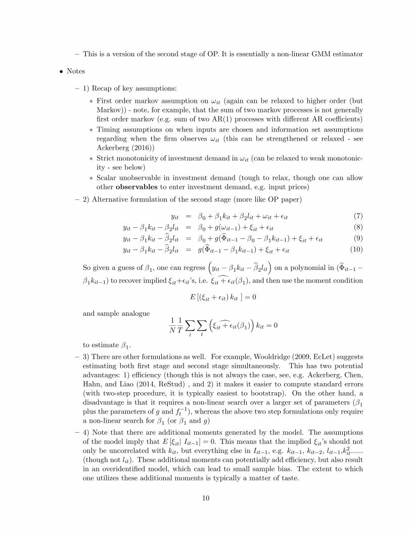
—This is a version of the second stage of OP. It is essentially a non-linear GMM estimator

• Notes

— 1) Recap of key assumptions:

∗ First order markov assumption on ωit (again can be relaxed to higher order (butMarkov)) - note, for example, that the sum of two markov processes is not generallyfirst order markov (e.g. sum of two AR(1) processes with different AR coeffi cients)∗ Timing assumptions on when inputs are chosen and information set assumptionsregarding when the firm observes ωit (this can be strengthened or relaxed - seeAckerberg (2016))∗ Strict monotonicity of investment demand in ωit (can be relaxed to weak monotonic-ity - see below)∗ Scalar unobservable in investment demand (tough to relax, though one can allowother observables to enter investment demand, e.g. input prices)

— 2) Alternative formulation of the second stage (more like OP paper)

yit = β0 + β1kit + β2lit + ωit + εit (7)

yit − β1kit − β2lit = β0 + g(ωit−1) + ξit + εit (8)

yit − β1kit − β2lit = β0 + g(Φit−1 − β0 − β1kit−1) + ξit + εit (9)

yit − β1kit − β2lit = g(Φit−1 − β1kit−1) + ξit + εit (10)

So given a guess of β1, one can regress(yit − β1kit − β2lit

)on a polynomial in (Φit−1−

β1kit−1) to recover implied ξit+εit’s, i.e. ξit + εit(β1), and then use the moment condition

E [(ξit + εit) kit ] = 0

and sample analogue1

N

1

T

∑i

∑t

( ξit + εit(β1))kit = 0

to estimate β1.

— 3) There are other formulations as well. For example, Wooldridge (2009, EcLet) suggestsestimating both first stage and second stage simultaneously. This has two potentialadvantages: 1) effi ciency (though this is not always the case, see, e.g. Ackerberg, Chen,Hahn, and Liao (2014, ReStud) , and 2) it makes it easier to compute standard errors(with two-step procedure, it is typically easiest to bootstrap). On the other hand, adisadvantage is that it requires a non-linear search over a larger set of parameters (β1plus the parameters of g and f−1t ), whereas the above two step formulations only requirea non-linear search for β1 (or β1 and g)

— 4) Note that there are additional moments generated by the model. The assumptionsof the model imply that E [ξit| Iit−1] = 0. This means that the implied ξit’s should notonly be uncorrelated with kit, but everything else in Iit−1, e.g. kit−1, kit−2, lit−1,k2it......(though not lit). These additional moments can potentially add effi ciency, but also resultin an overidentified model, which can lead to small sample bias. The extent to whichone utilizes these additional moments is typically a matter of taste.

10

— 5) Intuitive description of identification

∗ First stage: Compare output of firms with same iit and kit (which imply the sameωit) , but different lit. This variation in lit is uncorrelated with the remainingunobservables determining yit (εit), and so it identifies the labor coeffi cient. (Butagain, see ACF section below)∗ Second stage: Compare output of firms with same ωit−1, but different kit’s (notethat firms can have the same ωit−1, but different iit−1 and kit−1).

yit − β2lit = β0 + β1kit + g(ωit−1) + ξit + εit

= β0 + β1kit + g(Φit−1 − β0 − β1kit−1) + ξit + εit

This variation in kit is uncorrelated with the remaining unobservables determiningyit (ξit and εit), so it identifies the capital coeffi cient (However, note that the "com-parison of firms with same ωit−1" depends on the parameters themselves, so this isnot completely transparent intuition)

— 6) OP also deal with a selection problem due to the fact that unproductive firms mayexit the market. The problem is that even if

E [ξit| kit] = 0

in the entire population of firms,

E [ξit| kit, still in sample at t] may not equal 0 and be a function of kit

Specifically, if a firm’s exit decision at t depends on ωit (and thus ξit), then this secondexpectation is likely > 0 and depends negatively on kit (since firms with higher kit’s maybe more apt to stay in the market for a given ωit or ξit). OP develop a selection correctionto correct for this, which I dont think I will go through (see ABBP for discussion). Onthe other hand, if exit decisions at t are made at time t − 1 (a timing assumption likethat already being made on capital), then there is no selection problem, since in thiscase the exit decision is just a function of Iit−1.

6 Levinsohn and Petrin (2003, ReStud)

• Levinsohn and Petrin worry about the assumption that investment is strictly monotonic inωit. Intuitively, this assumption implies that any two firms with the same kit and iit musthave the same ωit.

• But in many datasets, especially in developing countries, iit is often 0 (e.g. in LP’s Chileandataset, approximately 50% of observations have 0 investment)

• It seems like a strong assumption that all these firms have the same ωit (given kit). It seemsmore likely that there is some threshold ωit below which firms invest 0.

• One can extend OP to allow weak monotonicity for the observations where iit = 0, butthis requires discarding these observations from the analysis (Aside: in this case, there isno selection issue as long as one uses the second stage moment E [(ξit + εit) kit ] = 0 ratherthan E [ξitkit ] = 0 (see Gandhi, Navarro and Rivers (GNR, 2015)). This is because onecannot compute implied ξit’s for observations for which iit = 0 (but one can compute implied(ξit + εit) for these observations))

11

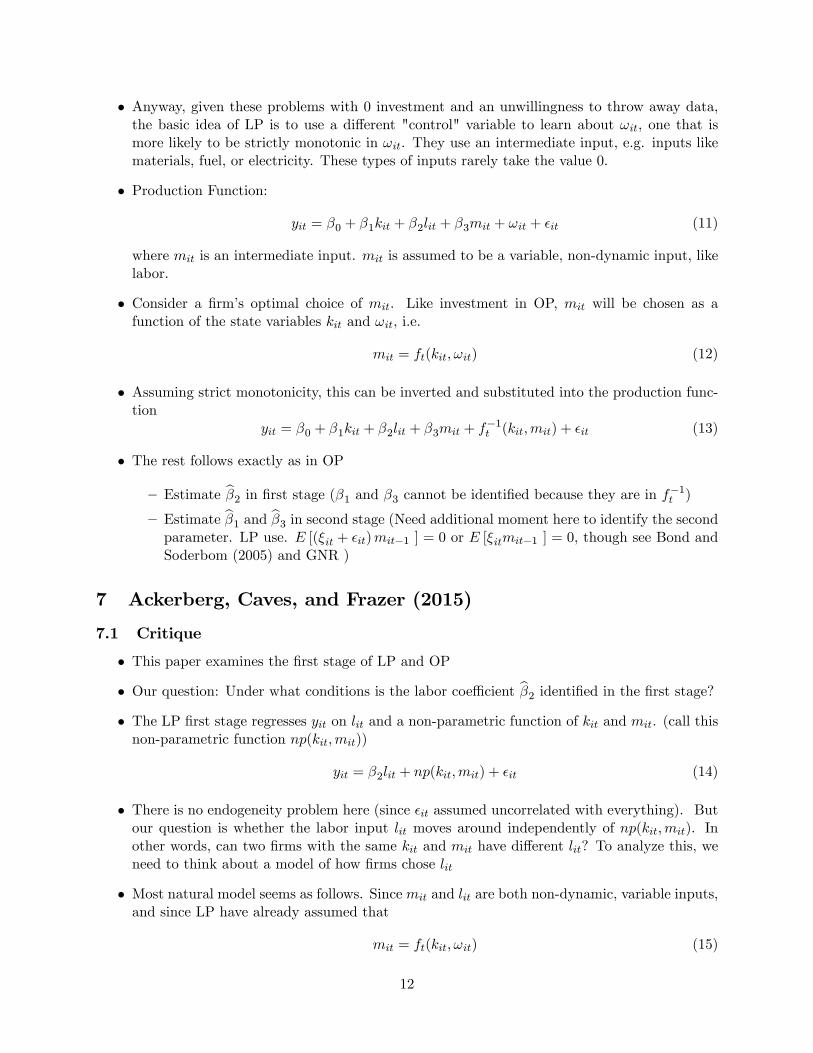
• Anyway, given these problems with 0 investment and an unwillingness to throw away data,the basic idea of LP is to use a different "control" variable to learn about ωit, one that ismore likely to be strictly monotonic in ωit. They use an intermediate input, e.g. inputs likematerials, fuel, or electricity. These types of inputs rarely take the value 0.

• Production Function:

yit = β0 + β1kit + β2lit + β3mit + ωit + εit (11)

where mit is an intermediate input. mit is assumed to be a variable, non-dynamic input, likelabor.

• Consider a firm’s optimal choice of mit. Like investment in OP, mit will be chosen as afunction of the state variables kit and ωit, i.e.

mit = ft(kit, ωit) (12)

• Assuming strict monotonicity, this can be inverted and substituted into the production func-tion

yit = β0 + β1kit + β2lit + β3mit + f−1t (kit,mit) + εit (13)

• The rest follows exactly as in OP

—Estimate β2 in first stage (β1 and β3 cannot be identified because they are in f−1t )

—Estimate β1 and β3 in second stage (Need additional moment here to identify the secondparameter. LP use. E [(ξit + εit)mit−1 ] = 0 or E [ξitmit−1 ] = 0, though see Bond andSoderbom (2005) and GNR )

7 Ackerberg, Caves, and Frazer (2015)

7.1 Critique

• This paper examines the first stage of LP and OP

• Our question: Under what conditions is the labor coeffi cient β2 identified in the first stage?

• The LP first stage regresses yit on lit and a non-parametric function of kit and mit. (call thisnon-parametric function np(kit,mit))

yit = β2lit + np(kit,mit) + εit (14)

• There is no endogeneity problem here (since εit assumed uncorrelated with everything). Butour question is whether the labor input lit moves around independently of np(kit,mit). Inother words, can two firms with the same kit and mit have different lit? To analyze this, weneed to think about a model of how firms chose lit

• Most natural model seems as follows. Sincemit and lit are both non-dynamic, variable inputs,and since LP have already assumed that

mit = ft(kit, ωit) (15)

12

it seems logical to treat lit symmetrically and assume

lit = ht(kit, ωit) (16)

Of course, these will be different functions.

• If this is the case, then note that

lit = ht(kit, ωit)

= ht(kit, f−1t (kit,mit))

= ht(kit,mit)

The last line implies that lit is a deterministic function of kit and mit

• But this is a problem for the first stage estimating equation

yit = β2lit + np(kit,mit) + εit (17)

since it implies that lit is functionally dependent on ("collinear" with) np(kit,mit), i.e. litdoesn’t move independently of np(kit,mit).

• Another way of saying this is as follows: LP want to condition on kit and mit (i.e. conditionon ωit) and look at remaining variation in lit to identify β2. But according to the above, litis a deterministic function of kit and mit. Hence, there is no remaining variation in lit oncewe condition on kit and mit!!!

• Can also think about both ht(kit,mit) and np(kit,mit) being polynomials.

• So if (16) is correct, then β2 should not be identified in the first stage. If OLS does in factproduce an estimate of β2, then some assumption of the model must be incorrect.

• To get the first stage of LP to work, we need to find something that moves around lit inde-pendently of np(kit,mit). Unfortunately, this is hard to do within the context of LP’s othermaintained assumptions. For example, suppose one assumes that there is some firm-specificunobserved shock to the price of labor, vit. This will clearly affect firms’optimal labor choices,i.e..

lit = ht(kit, ωit, vit)

The problem is that this will also generally affect the firms’optimal choice of materials

mit = ft(kit, ωit, , vit) (18)

which then violates the scalar unobservable assumption necessary to invert ft and write ωitas a function of observables.

• Our paper thinks about various alternative models of lit (i.e. various data-generating processes(DGPs)) that might "break" this functional dependence problem. We can only come up with2 such DGPs, and neither seems all that general.

13

• 1) Suppose there is "optimization" error in lit, i.e.

lit = ht(kit, ωit) + uit

where uit is independent of (kit, ωit). In other words i.e. for some exogenous reason firmsdo not get the optimal choice of labor correct. This breaks the functional dependence prob-lem (and does not seem completely unreasonable). On the other hand, one simultaneouslyneeds to assume that there is 0 optimization error in mit (otherwise, the scalar unobservableassumption is violated). It seems challenging to argue that there is a significant amount ofoptimization error in lit, but almost no optimization error in mit. (One example might be ifone’s data measures "planned" or ordered materials, but actual labor (e.g. subject to sickdays or unexpected quits))

• 2) Suppose that mit is chosen at some point in time prior to lit, and that:

— a) The firm knows ωit when choosing mit

— b) Between these two points in time, there is a shock to the price of labor, vit, that variesacross firms.

— c) vit is independent across time (and other variables in the model)

• This second DGP also allows the labor coeffi cient to be identified in the first stage, because theshock vit moves lit around conditional on mit and kit. Note that vit needs to be independentacross time, otherwise the choice of mit at t will optimally depend on vit−1, violating thescalar unobservable assumption needed for invertibility.

• Again, this DGP does not seem very general. Why is mit chosen before lit (if anything, Iwould tend to think the reverse)? And it seems like a stretch to assume that there are nounobserved firm specific input price shocks except for this very special vit shock that must berealized between these two points in time.

• Notes:

• 1) Parametric treatment of the intermediate input demand function does not rescue the LPfirst stage identification - see ACF for details (though unlike with iit it is not hard to do this,and it likely adds effi ciency)

• 2) The OP estimator is also affected by this critique. However, there is a 3rd DGP thatbreaks the functional dependence problem. This involves lit being chosen with incompleteknowledge of ωit, e.g. prior to the realization of ωit - see ACF for details.

• 3)Bond and Soderbom (2005) make a related argument that criticizes the second stage iden-tification of β3 (the coeffi cient on the intermediate input) in LP. The crux of the implicationsof their argument is that under the assumptions of the LP model the moment conditionE [(ξit + εit)mit−1 ] = 0 or E [ξitmit−1 ] = 0 is not informative about the coeffi cient β3. Theintuition is that under the assumptions of the LP model, mit−1 is not correlated with mit

conditional on kit and ωit−1- hence it is uninformative as an instrument. A serially corre-lated, firm-specific, unobserved price shock to the intermediate input could generate suchcorrelation, but it violates the LP scalar unobservable assumption. More generally, Bondand Soderbom show that without firm specific input price variation, coeffi cients on perfectly

14

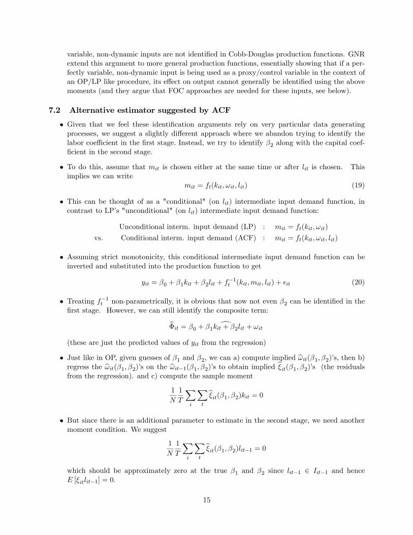
variable, non-dynamic inputs are not identified in Cobb-Douglas production functions. GNRextend this argument to more general production functions, essentially showing that if a per-fectly variable, non-dynamic input is being used as a proxy/control variable in the context ofan OP/LP like procedure, its effect on output cannot generally be identified using the abovemoments (and they argue that FOC approaches are needed for these inputs, see below).

7.2 Alternative estimator suggested by ACF

• Given that we feel these identification arguments rely on very particular data generatingprocesses, we suggest a slightly different approach where we abandon trying to identify thelabor coeffi cient in the first stage. Instead, we try to identify β2 along with the capital coef-ficient in the second stage.

• To do this, assume that mit is chosen either at the same time or after lit is chosen. Thisimplies we can write

mit = ft(kit, ωit, lit) (19)

• This can be thought of as a "conditional" (on lit) intermediate input demand function, incontrast to LP’s "unconditional" (on lit) intermediate input demand function:

Unconditional interm. input demand (LP) : mit = ft(kit, ωit)

vs. Conditional interm. input demand (ACF) : mit = ft(kit, ωit, lit)

• Assuming strict monotonicity, this conditional intermediate input demand function can beinverted and substituted into the production function to get

yit = β0 + β1kit + β2lit + f−1t (kit,mit, lit) + εit (20)

• Treating f−1t non-parametrically, it is obvious that now not even β2 can be identified in thefirst stage. However, we can still identify the composite term:

Φit = β0 + β1kit + β2lit + ωit

(these are just the predicted values of yit from the regression)

• Just like in OP, given guesses of β1 and β2, we can a) compute implied ωit(β1, β2)’s, then b)regress the ωit(β1, β2)’s on the ωit−1(β1, β2)’s to obtain implied ξit(β1, β2)’s (the residualsfrom the regression). and c) compute the sample moment

1

N

1

T

∑i

∑t

ξit(β1, β2)kit = 0

• But since there is an additional parameter to estimate in the second stage, we need anothermoment condition. We suggest

1

N

1

T

∑i

∑t

ξit(β1, β2)lit−1 = 0

which should be approximately zero at the true β1 and β2 since lit−1 ∈ Iit−1 and henceE [ξitlit−1] = 0.

15

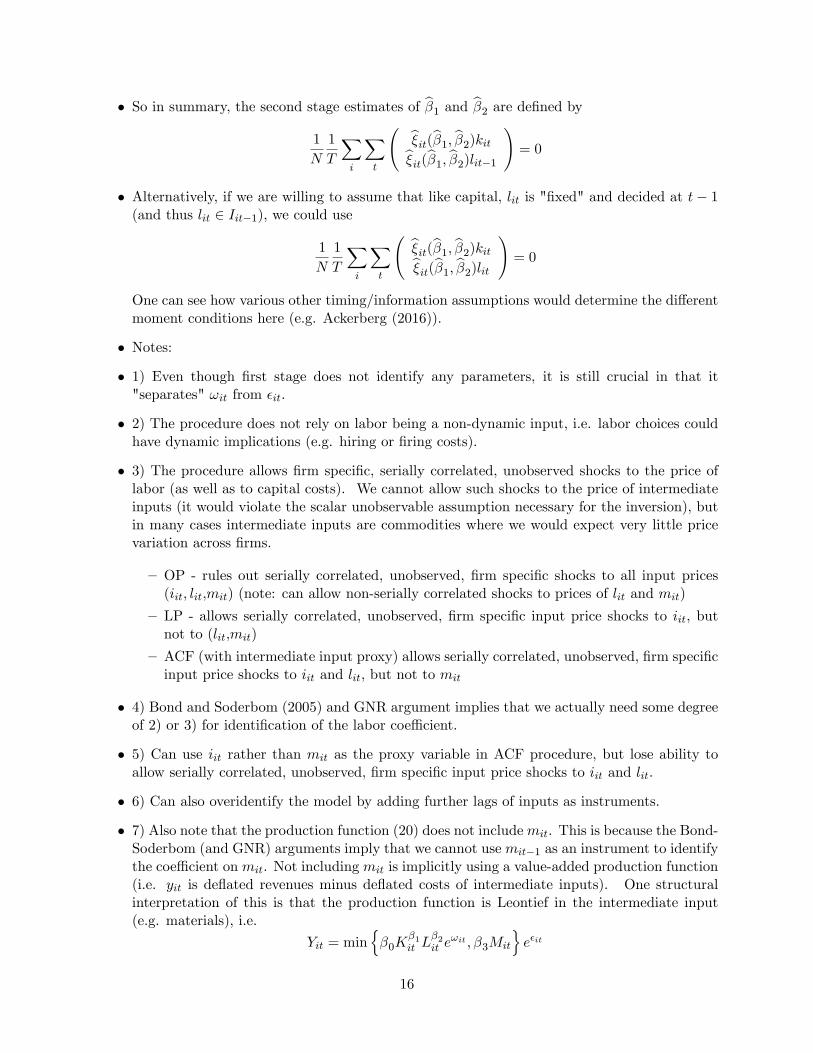
• So in summary, the second stage estimates of β1 and β2 are defined by

1

N

1

T

∑i

∑t

(ξit(β1, β2)kitξit(β1, β2)lit−1

)= 0

• Alternatively, if we are willing to assume that like capital, lit is "fixed" and decided at t− 1(and thus lit ∈ Iit−1), we could use

1

N

1

T

∑i

∑t

(ξit(β1, β2)kitξit(β1, β2)lit

)= 0

One can see how various other timing/information assumptions would determine the differentmoment conditions here (e.g. Ackerberg (2016)).

• Notes:

• 1) Even though first stage does not identify any parameters, it is still crucial in that it"separates" ωit from εit.

• 2) The procedure does not rely on labor being a non-dynamic input, i.e. labor choices couldhave dynamic implications (e.g. hiring or firing costs).

• 3) The procedure allows firm specific, serially correlated, unobserved shocks to the price oflabor (as well as to capital costs). We cannot allow such shocks to the price of intermediateinputs (it would violate the scalar unobservable assumption necessary for the inversion), butin many cases intermediate inputs are commodities where we would expect very little pricevariation across firms.

—OP - rules out serially correlated, unobserved, firm specific shocks to all input prices(iit, lit,mit) (note: can allow non-serially correlated shocks to prices of lit and mit)

— LP - allows serially correlated, unobserved, firm specific input price shocks to iit, butnot to (lit,mit)

—ACF (with intermediate input proxy) allows serially correlated, unobserved, firm specificinput price shocks to iit and lit, but not to mit

• 4) Bond and Soderbom (2005) and GNR argument implies that we actually need some degreeof 2) or 3) for identification of the labor coeffi cient.

• 5) Can use iit rather than mit as the proxy variable in ACF procedure, but lose ability toallow serially correlated, unobserved, firm specific input price shocks to iit and lit.

• 6) Can also overidentify the model by adding further lags of inputs as instruments.

• 7) Also note that the production function (20) does not includemit. This is because the Bond-Soderbom (and GNR) arguments imply that we cannot usemit−1 as an instrument to identifythe coeffi cient on mit. Not including mit is implicitly using a value-added production function(i.e. yit is deflated revenues minus deflated costs of intermediate inputs). One structuralinterpretation of this is that the production function is Leontief in the intermediate input(e.g. materials), i.e.

Yit = min{β0K

β1it L

β2it e

ωit , β3Mit

}eεit

16

which implies thatyit = β0 + β1kit + β2lit + ωit + εit (21)

An alternative would be to follow Appendix B of Levinsohn and Petrin, or Gandhi, Navarroand Rivers (2015) and use a first order condition to obtain the coeffi cient on the intermediateinput.

• 8) Less parametric generalizations

—Ackerberg and Hahn (2015) show that in this "value added model"

Yit = min {F (Kit, Lit, ωit) , β3Mit} eεit

yit = min {f(kit, lit, ωit), ln(β3) +mit}+ εit

if f is strictly monotonic in the scalar markov process ωit, it can be fully non-parametricallyidentified. We formally consider the generic model yit = f (xit, ωit) and show conditionson timing and information sets under which f is non-parametrically identified. Wedescribe the result as showing how the timing/information set assumptions crucial toOP have power in a non-parametric context. Note that these assumptions are startingto be used in other literatures, e.g. demand with endogenous product characteristics.

—Gandhi, Navarro and Rivers (2015) extend the first order condition approach to esti-mating the effect of the proxy variable (mit) to a non-parametric setting and show thatin

yit = f(kit, lit,mit) + ωit + εit

f is non-parametrically identified. I would describe this approach as combining thetiming/information set assumption identification approach (for kit and lit) with the firstorder condition identification approach (for mit)

• 9) More generally can mix-and-match the different identification strategies (for different in-puts), i.e.

— timing/information set assumptions (though as detailed above, this does not work for anon-dynamic, variable inputs that is being used to proxy for unobserved productivity).

—first order conditions (at least for static inputs)

— observed firm specific input price shocks as instruments

8 Dynamic Panel Approaches

• These are econometric procedures (Arellano and Bond (1991, ReStud), Arellano and Bover(1995. JoE), Blundell and Bond (1998, JoE, 2000, ER), Arellano and Honore (2001, Hand-book)) that generalize the fixed effects model to allow ωit to vary across time. These havebeen used in many different applied contexts, including production functions (e.g. BlundellBond 2000, and emprical work by John Van Reenan, Nick Bloom and coauthors).

• "Dynamic Panel" is somewhat of a misnomer in the context that I am using these methodolo-gies, as there is no lagged dependent r.h.s. variable. Many of these methods were developedin that context.

17

• I will focus on one very simple example, to try to highlight the similarities and differencesbetween this literature and the literature stemming from OP.

• Production functionyit = β0 + β1kit + β2lit + ωit + εit (22)

whereωit = ρωit−1 + ξit

• Suppose that εit satisfies strict exogeneity, i.e. εit’s are uncorrelated with all input choices.

• Suppose that ωit not observed until t, that kit is chosen at t− 1, and that lit is chosen at t.

• These assumptions are analagous to the timing/information set assumptions made in OP,and imply the following orthogonality conditions

E [εitkis] = E [εitlis] = 0 ∀t, sE [ξitkis] = 0 for s ≤ tE [ξitlis] = 0 for s < t

• Consider "ρ-differencing" the production function, i.e.

yit − ρyit−1 = (1− ρ)β0 + β1 (kit − ρkit−1) + β2 (lit − ρlit−1) + ξit + (εit − ρεit−1)

or

yit = ρyit−1 + (1− ρ)β0 + β1 (kit − ρkit−1) + β2 (lit − ρlit−1) + ξit + (εit − ρεit−1)

• Now, given a guess of the parameters (ρ, β0, β1, β2) one can compute the implied values ofthe term ξit + (εit − ρεit−1), i.e.

ξit + (εit − ρεit−1) (ρ, β0, β1, β2) = yit−ρyit−1− (1−ρ)β0−β1 (kit − ρkit−1)−β2 (lit − ρlit−1)

Then estimation can proceed using, e.g. by setting the sample moment

1

N

1

T

∑i

∑t

ξit + (εit − ρεit−1) (ρ, β0, β1, β2)⊗

1kitkit−1lit−1

= 0−→

• Again, there are actually many more potential moment conditions, since all values of k, l, andy prior to (kit, lit−1, yit−2) are also uncorrelated with ξit + (εit − ρεit−1).

• Note:

—There are implicit assumptions here about what makes lags strong instruments. Thisdepends on dynamic issues (e.g. adjustment costs) and issues regarding serial correla-tion in input prices. See Blundell and Bond (1999) and Bond and Soderbom (2005)for discussion of when they are strong instruments, and when they are not so stronginstruments.

18

—One can extend the model to allow for an additional unobservable that is fixed acrosstime, i.e.

yit = β0 + β1kit + β2lit + αi + ωit + εit (23)

where αi is allowed to be correlated with all input choices. This model requires "doubledifferencing", i.e.

(yit − ρyit−1)− (yit−1 − ρyit−2) = β1 [(kit − ρkit−1)− (kit−1 − ρkit−2)] + β2 [(lit − ρlit−1)− (lit−1 − ρlit−2)]+ξit − ξit−1 + (εit − ρεit−1)− (εit−1 − ρεit−2)

Again, one can appropriately lag k, l, and y to find valid moments. One problem isthat double differencing can be demanding on the data, and estimates can be imprecise.Arellano and Bover (1995) and Blundell and Bond (1998, 2000) suggest some additionalmoment conditions based on stationarity assumptions that can help here, though theseassumptions may be strong.

• So how do these dynamic panel approaches compare to the Olley-Pakes literature? I’d saythe main tradeoff is the following

—The dynamic panel approach does not require the scalar unobservable and strict monotonic-ity assumptions that are required for the OP/LP/ACF inversions. So in the dynamicpanel literature, for example, one does not need to worry about unobserved firm specificinput prices, nor other sorts of unobservables like optimization error.

—On the other hand, the dynamic panel approach requires that the serial correlation inωit is linear, e.g. an AR or MA process. This is essential to being able to constructusable moments. In contrast, the OP/LP/ACF literature can allow the productivityshock to follow a completely general first order markov process.

—Dynamic panel literature can also allow additional fixed effects, although precise estima-tion appears to be challenging. Intermediate assumption of Arellano-Bover Blundell-Bover may be helpful.

• Given that theory may provide little guidance between choosing between these two sets ofassumptions (and because they are both strong), I would suggest trying both approaches.

9 Other Issues

• 1) Often observe firm revenues as the output measure, not physical quantities. As pointed outby Klette and Griliches (1996, JAE), this can be problematic when firms operate in distinctimperfectly competitive output markets (and one does not observe output price).

— Intuition: Suppose observe that firms that (exogenously) use double the inputs of othersproduce less than double revenue of other. There are two explanations - 1) decliningreturns to scale (but, e.g., perfect competition), 2) constant returns to scale with adownward sloping demand curve.

—Even if one doesn’t care about separating the above two effects, there may now be twodistinct sources of unobservables in the (revenue) production function, which can beproblematic for the proxy based approaches.

19

— See, e.g. Klette (1999, JIE), Foster, Haltiwanger, and Syverson (2007, AER), DeLoecker(2011, Ecta), DeLoecker and Warzynski (2012, AER).

—Note that just observing quantites is not a complete panacea - need to be equivalentacross firms for these quantities to be meaningful.

• 2) Other types of information structures (e.g. Greenstreet (2007)).

• 3) Additional inputs (e.g. Griliches Knowledge Capital model, Doraszelski and Jaumandreu(2014, ReStud))

—Griliches Knowledge capital

yit = β0 + β1kit + β2lit + β3cit + ωit + εit (24)

where

cit =t∑

τ=0

δt−τc diτ

where diτ is firm’s chosen R&D expenditures in period τ

—Doraszelski and Jaumandreu (2014)

yit = β0 + β1kit + β2lit + ωit + εit (25)

whereωit = g(ωit−1, dit−1)

—Advantages DJ

∗ Doesn’t have has initial t = 0 R&D stock issue that Griliches has (assuming useOP/LP/ACF related methods to estimate)∗ Explicitly has uncertainty in the contribution of R&D to productivity

—Disadvantages DJ

∗ Unobserved component of "productivity" and R&D component of "productivity"affect future through scalar - this is restrictive, e.g.

ωit = ρωit−1 + dit−1 + ξit

dit−1 and ξit forced to depreciate at same rate. This is not the case in Griliches -i.e. δc different than ρ.∗ Alternative model of physical capital stock

yit = β0 + β2lit + ωit + εit (26)

whereωit = g(ωit−1, dit−1, iit−1)

—Note: both "endogenize productivity" if think about defining productivity as (β3cit+ωit)in the Griliches model

• 4) Empirical questions -

20

—Determinants of productivity - deregulation (OP), trade openess, exporting - similar toabove

∗ generally best to include these factors as inputs in the production function—Allocative effi ciency - recently Hsieh and Klenow (2009, QJE), Asker, Collard-Wexler,and DeLoecker (2014, JPE)

21